Tag Archives: TensorFlow

Advances in TF-Ranking

In December 2018, we introduced TF-Ranking, an open-source TensorFlow-based library for developing scalable neural learning-to-rank (LTR) models, which are useful in settings where users expect to receive an ordered list of items in response to their query. LTR models — unlike standard classification models that classify one item at a time — receive an entire list of items as an input, and learn an ordering that maximizes the utility of the entire list. While search and recommendation systems are the most common applications of LTR models, since its release, we have seen TF-Ranking being applied in diverse domains beyond search, including e-commerce, SAT solvers, and smart city planning.

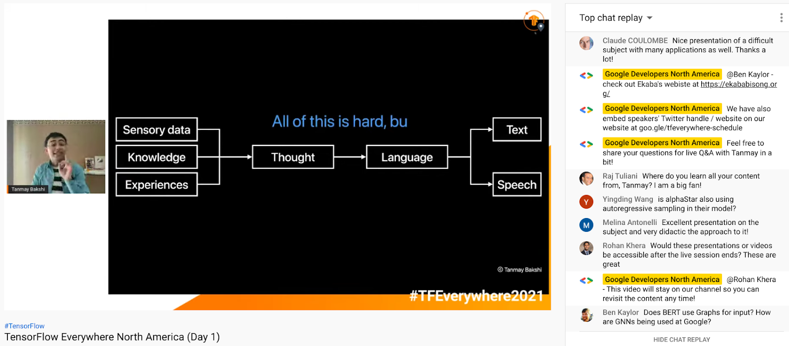
The goal of learning-to-rank (LTR) is to learn a function f() that takes as an input a list of items (documents, products, movies, etc.) and outputs the list of items in the optimal order (descending order of relevance). Here, green shade indicates item relevance level, and the red item marked with 'x' is non-relevant.

In May 2021, we published a major release of TF-Ranking that enables full support for natively building LTR models using Keras, a high-level API of TensorFlow 2. Our native Keras ranking model has a brand-new workflow design, including a flexible ModelBuilder, a DatasetBuilder to set up training data, and a Pipeline to train the model with the provided dataset. These components make building a customized LTR model easier than ever, and facilitate rapid exploration of new model structures for production and research. If RaggedTensors are your tool of choice, TF-Ranking is now working with them as well. In addition, our most recent release, which incorporates the Orbit training library, contains a long list of advances — the culmination of two and half years of neural LTR research. Below we share a few of the key improvements available in the latest TF-Ranking version.

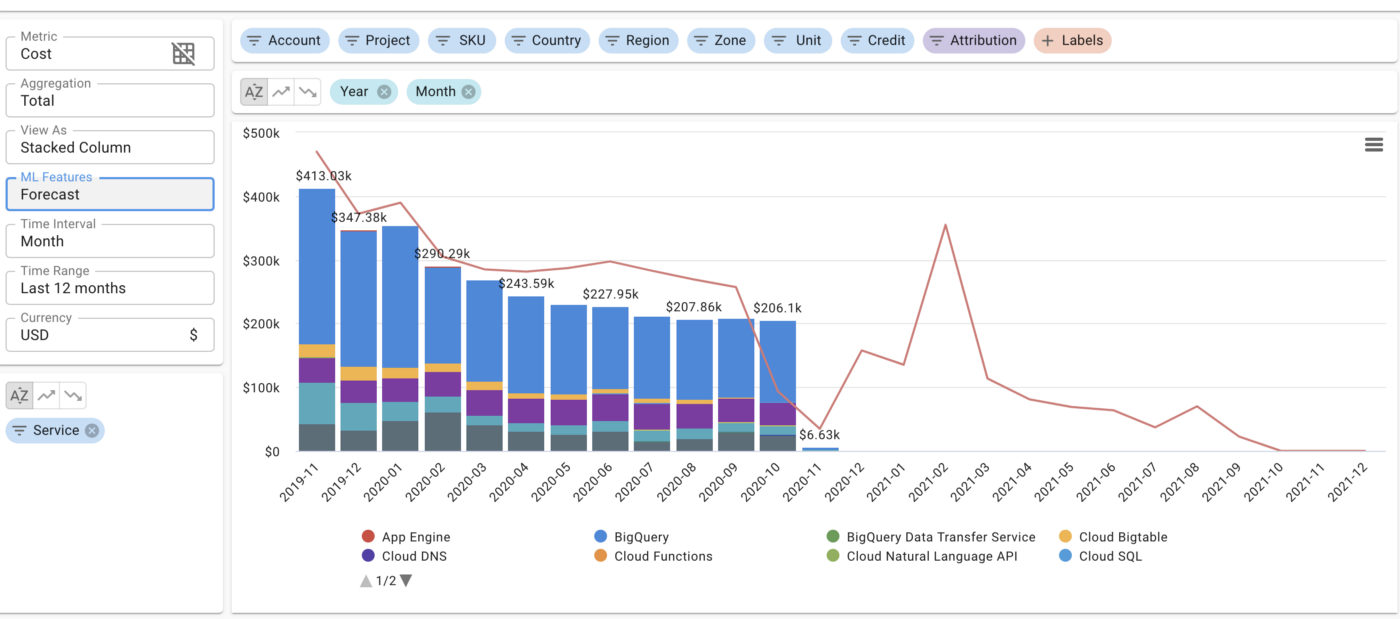
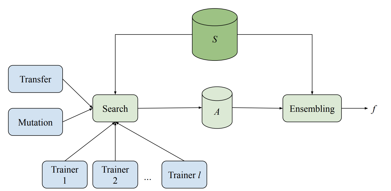
Workflow to build and train a native Keras ranking model. Blue modules are provided by TF-Ranking, and green modules are customizable.

Learning-to-Rank with TFR-BERT
Recently, pretrained language models like BERT have achieved state-of-the-art performance on various language understanding tasks. To capture the expressiveness of these models, TF-Ranking implements a novel TFR-BERT architecture that couples BERT with the power of LTR to optimize the ordering of list inputs. As an example, consider a query and a list of n documents that one might like to rank in response to this query. Instead of learning an independent BERT representation for each <query, document> pair, LTR models apply a ranking loss to jointly learn a BERT representation that maximizes the utility of the entire ranked list with respect to the ground-truth labels.

The figure below illustrates this process. First, we flatten a list of n documents to rank in response to a query into a list <query, document> tuples. These tuples are fed into a pre-trained language model (e.g., BERT). The pooled BERT outputs for the entire document list are then jointly fine-tuned with one of the specialized ranking losses available in TF-Ranking. Our experience shows that this TFR-BERT architecture delivers significant improvements in pretrained language model performance, leading to state-of-the-art performance for several popular ranking tasks, especially when multiple pretrained language models are ensembled. Our users can now get started with TFR-BERT using this simple example.

An illustration of the TFR-BERT architecture, in which a joint LTR model over a list of n documents is constructed using BERT representations of individual <query, document> pairs.

Interpretable Learning-to-Rank
Transparency and interpretability are important factors in deploying LTR models in ranking systems that can be involved in determining the outcomes of processes such as loan eligibility assessment, advertisement targeting, or guiding medical treatment decisions. In such cases, the contribution of each individual feature to the final ranking should be examinable and understandable to ensure transparency, accountability and fairness of the outcomes.

One possible way to achieve this is using generalized additive models (GAMs) — intrinsically interpretable machine learning models that are linearly composed of smooth functions of individual features. However, while GAMs have been extensively studied on regression and classification tasks, it is less clear how to apply them in a ranking setting. For instance, while GAMs can be straightforwardly applied to model each individual item in the list, modeling both item interactions and the context in which these items are ranked is a more challenging research problem. To this end, we have developed a neural ranking GAM — an extension of generalized additive models to ranking problems.

Unlike standard GAMs, a neural ranking GAM can take into account both the features of the ranked items and the context features (e.g., query or user profile) to derive an interpretable, compact model. This ensures that not only the contribution of each item-level feature is interpretable, but also the contribution of the context features. For example, in the figure below, using a neural ranking GAM makes visible how distance, price, and relevance, in the context of a given user device, contribute to the final ranking of the hotel. Neural ranking GAMs are now available as a part of TF-Ranking,

An example of applying neural ranking GAM for local search. For each input feature (e.g., price, distance), a sub-model produces a sub-score that can be examined, providing transparency. Context features (e.g., user device type) can be utilized to derive importance weights of submodels.

Neural Ranking or Gradient Boosting?
While neural models have achieved state of the art performance in multiple domains, specialized gradient boosted decision trees (GBDTs) like LambdaMART remained the baseline to beat in a variety of open LTR datasets. The success of GBDTs in open datasets is due to several reasons. First, due to their relatively small size, neural models are prone to overfitting on these datasets. Second, since GBDTs partition their input feature space using decision trees, they are naturally more resilient to variations in numerical scales in ranking data, which often contain features with Zipfian or otherwise skewed distributions. However, GBDTs do have their limitations in more realistic ranking scenarios, which often combine both textual and numerical features. For instance, GBDTs cannot be directly applied to large discrete feature spaces, such as raw document text. They are also, in general, less scalable than neural ranking models.

Therefore, since the TF-Ranking release, our team has significantly deepened the understanding of how best to leverage neural models in ranking with numerical features. This culminated in a Data Augmented Self-Attentive Latent Cross (DASALC) model, described in an ICLR 2021 paper, which is the first to establish parity, and in some cases statistically significant improvements, of neural ranking models over strong LambdaMART baselines on open LTR datasets. This achievement is made possible through a combination of techniques, which include data augmentation, neural feature transformation, self-attention for modeling document interactions, listwise ranking loss, and model ensembling similar to boosting in GBDTs. The architecture of the DASALC model was entirely implemented using the TF-Ranking library.

Conclusion
All in all, we believe that the new Keras-based TF-Ranking version will make it easier to conduct neural LTR research and deploy production-grade ranking systems. We encourage everyone to try out the latest version and follow this introductory example for a hands-on experience. While we are very excited about this new release, our research and development journey is far from over, so we will continue to advance our understanding of learning-to-rank problems and share these advances with our users.

Acknowledgements
This project was only possible thanks to the current and past members of the TF-Ranking team: Honglei Zhuang, ‎Le Yan, Rama Pasumarthi, Rolf Jagerman, Zhen Qin, Shuguang Han, Sebastian Bruch, Nathan Cordeiro, Marc Najork and Patrick McGregor. We also extend special thanks to our collaborators from the Tensorflow team: Zhenyu Tan, Goldie Gadde, Rick Chao, Yuefeng Zhou‎, Hongkun Yu, and Jing Li.

Source: Google AI Blog


Announcing Android’s updateable, fully integrated ML inference stack

Posted by Oli Gaymond, Product Manager, Android ML

On-Device Machine Learning provides lower latency, more efficient battery usage, and features that do not require network connectivity. We have found that development teams deploying on-device ML on Android today encounter these common challenges:

  • Many apps are size constrained, so having to bundle and manage additional libraries just for ML can be a significant cost
  • Unlike server-based ML, the compute environment is highly heterogeneous, resulting in significant differences in performance, stability and accuracy
  • Maximising reach can lead to using older more broadly available APIs; which limits usage of the latest advances in ML.

To help solve these problems, we’ve built Android ML Platform - an updateable, fully integrated ML inference stack. With Android ML Platform, developers get:

  • Built in on-device inference essentials - we will provide on-device inference binaries with Android and keep them up to date; this reduces apk size
  • Optimal performance on all devices - we will optimize the integration with Android to automatically make performance decisions based on the device, including enabling hardware acceleration when available
  • A consistent API that spans Android versions - regular updates are delivered via Google Play Services and are made available outside of the Android OS release cycle

Built in on-device inference essentials - TensorFlow Lite for Android

TensorFlow Lite will be available on all devices with Google Play Services. Developers will no longer need to include the runtime in their apps, reducing app size. Moreover, TensorFlow Lite for Android will use metadata in the model to automatically enable hardware acceleration, allowing developers to get the best performance possible on each Android device.

Optimal performance on all devices - Automatic Acceleration

Automatic Acceleration is a new feature in TensorFlowLite for Android. It enables per-model testing to create allowlists for specific devices taking performance, accuracy and stability into account. These allowlists can be used at runtime to decide when to turn on hardware acceleration. In order to use accelerator allowlisting, developers will need to provide additional metadata to verify correctness. Automatic Acceleration will be available later this year.

A consistent API that spans Android versions

Besides keeping TensorFlow Lite for Android up to date via regular updates, we’re also going to be updating the Neural Networks API outside of OS releases while keeping the API specification the same across Android versions. In addition we are working with chipset vendors to provide the latest drivers for their hardware directly to devices, outside of OS updates. This will let developers dramatically reduce testing from thousands of devices to a handful of configurations. We’re excited to announce that we’ll be launching later this year with Qualcomm as our first partner.

Sign-up for our early access program

While several of these features will roll out later this year, we are providing early access to TensorFlow Lite for Android to developers who are interested in getting started sooner. You can sign-up for our early access program here.

Developer updates from Coral

Posted by The Coral Team

We're always excited to share updates to our Coral platform for building edge ML applications. In this post, we have some interesting demos, interfaces, and tutorials to share, and we'll start by pointing you to an important software update for the Coral Dev Board.

Important update for the Dev Board / SoM

If you have a Coral Dev Board or Coral SoM, please install our latest Mendel update as soon as possible to receive a critical fix to part of the SoC power configuration. To get it, just log onto your board and install the update as follows:

Dev Board / Som

This will install a patch from NXP for the Dev Board / SoM's SoC, without which it's possible the SoC will overstress and the lifetime of the device could be reduced. If you recently flashed your board with the latest system image, you might already have this fix (we also updated the flashable image today), but it never hurts to fetch all updates, as shown above.

Note: This update does not apply to the Dev Board Mini.


Manufacturing demo

We recently published the Coral Manufacturing Demo, which demonstrates how to use a single Coral Edge TPU to simultaneously accomplish two common manufacturing use-cases: worker safety and visual inspection.

The demo is designed for two specific videos and tasks (worker keepout detection and apple quality grading) but it is designed to be easily customized with different inputs and tasks. The demo, written in C++, requires OpenGL and is primarily targeted at x86 systems which are prevalent in manufacturing gateways – although ARM Cortex-A systems, like the Coral Dev Board, are also supported.

demo image

Web Coral

We've been working hard to make ML acceleration with the Coral Edge TPU available for most popular systems. So we're proud to announce support for WebUSB, allowing you to use the Coral USB Accelerator directly from Chrome. To get started, check out our WebCoral demo, which builds a webpage where you can select a model and run an inference accelerated by the Edge TPU.

 Edge TPU

New models repository

We recently released a new models repository that makes it easier to explore the various trained models available for the Coral platform, including image classification, object detection, semantic segmentation, pose estimation, and speech recognition. Each family page lists the various models, including details about training dataset, input size, latency, accuracy, model size, and other parameters, making it easier to select the best fit for the application at hand. Lastly, each family page includes links to training scripts and example code to help you get started. Or for an overview of all our models, you can see them all on one page.

Models, trained TensorFlow models for the Edge TPU

Transfer learning tutorials

Even with our collection of pre-trained models, it can sometimes be tricky to create a task-specific model that's compatible with our Edge TPU accelerator. To make this easier, we've released some new Google Colab tutorials that allow you to perform transfer learning for object detection, using MobileDet and EfficientDet-Lite models. You can find these and other Colabs in our GitHub Tutorials repo.

We are excited to share all that Coral has to offer as we continue to evolve our platform. Keep an eye out for more software and platform related news coming this summer. To discover more about our edge ML platform, please visit Coral.ai and share your feedback at [email protected].

Machine Learning GDEs: Q1 2021 highlights, projects and achievements

Posted by HyeJung Lee and MJ You, Google ML Ecosystem Community Managers. Reviewed by Soonson Kwon, Developer Relations Program Manager.

Google Developers Experts is a community of passionate developers who love to share their knowledge with others. Many of them specialize in Machine Learning (ML). Despite many unexpected changes over the last months and reduced opportunities for various in person activities during the ongoing pandemic, their enthusiasm did not stop.

Here are some highlights of the ML GDE’s hard work during the Q1 2021 which contributed to the global ML ecosystem.

ML GDE YouTube channel

ML GDE YouTube page

With the initiative and lead of US-based GDE Margaret Maynard-Reid, we launched the ML GDEs YouTube channel. It is a great way for GDEs to reach global audiences, collaborate as a community, create unique content and promote each other's work. It will contain all kinds of ML related topics: talks on technical topics, tutorials, interviews with another (ML) GDE, a Googler or anyone in the ML community etc. Many videos have already been uploaded, including: ML GDE’s intro from all over the world, tips for TensorFlow & GCP Certification and how to use Google Cloud Platform etc. Subscribe to the channel now!!

TensorFlow Everywhere

TensorFlow Everywhere logo

17 ML GDEs presented at TensorFlow Everywhere (a global community-led event series for TensorFlow and Machine Learning enthusiasts and developers around the world) hosted by local TensorFlow user groups. You can watch the recorded sessions in the TensorFlow Everywhere playlist on the ML GDE Youtube channel. Most of the sessions cover new features in Tensorflow.

International Women’s Day

Many ML GDEs participated in activities to celebrate International Women’s Day (March 8th). GDE Ruqiya Bin Safi (based in Saudi Arabia) cooperated with WTM Saudi Arabia to organize “Socialthon” - social development hackathons and gave a talk “Successful Experiences in Social Development", which reached 77K viervers live and hit 10K replays. India-based GDE Charmi Chokshi participated in GirlScript's International Women's Day event and gave a talk: “Women In Tech and How we can help the underrepresented in the challenging world”. If you’re looking for more inspiring materials, check out the “Women in AI” playlist on our ML GDE YouTube channel!

Mentoring

ML GDEs are also very active in mentoring community developers, students in the Google Developer Student Clubs and startups in the Google for Startups Accelerator program. Among many, GDE Arnaldo Gualberto (Brazil) conducted mentorship sessions for startups in the Google Fast Track program, discussing how to solve challanges using Machine Learning/Deep Learning with TensorFlow.

TensorFlow

Practical Adversarial Robustness in Deep Learning: Problems and Solutions
ML using TF cookbook and ML for Dummies book

Meanwhile in Europe, GDEs Alexia Audevart (based in France) and Luca Massaron (based in Italy) released “Machine Learning using TensorFlow Cookbook”. It provides simple and effective ideas to successfully use TensorFlow 2.x in computer vision, NLP and tabular data projects. Additionally, Luca published the second edition of the Machine Learning For Dummies book, first published in 2015. Her latest edition is enhanced with product updates and the principal is a larger share of pages devoted to discussion of Deep Learning and TensorFlow / Keras usage.

YouTube video screenshot

On top of her women-in-tech related activities, Ruqiya Bin Safi is also running a “Welcome to Deep Learning Course and Orientation” monthly workshop throughout 2021. The course aims to help participants gain foundational knowledge of deep learning algorithms and get practical experience in building neural networks in TensorFlow.

TensorFlow Project showcase

Nepal-based GDE Kshitiz Rimal gave a talk “TensorFlow Project Showcase: Cash Recognition for Visually Impaired" on his project which uses TensorFlow, Google Cloud AutoML and edge computing technologies to create a solution for the visually impaired community in Nepal.

Screenshot of TF Everywhere NA talk

On the other side of the world, in Canada, GDE Tanmay Bakshi presented a talk “Machine Learning-powered Pipelines to Augment Human Specialists” during TensorFlow Everywhere NA. It covered the world of NLP through Deep Learning, how it's historically been done, the Transformer revolution, and how using the TensorFlow & Keras to implement use cases ranging from small-scale name generation to large-scale Amazon review quality ranking.

Google Cloud Platform

Google Cloud Platform YouTube playlist screenshot

We have been equally busy on the GCP side as well. In the US, GDE Srivatsan Srinivasan created a series of videos called “Artificial Intelligence on Google Cloud Platform”, with one of the episodes, "Google Cloud Products and Professional Machine Learning Engineer Certification Deep Dive", getting over 3,000 views.

ML Analysis Pipeline

Korean GDE Chansung Park contributed to TensorFlow User Group Korea with his “Machine Learning Pipeline (CI/CD for ML Products in GCP)” analysis, focused on about machine learning pipeline in Google Cloud Platform.

Analytics dashboard

Last but not least, GDE Gad Benram based in Israel wrote an article on “Seven Tips for Forecasting Cloud Costs”, where he explains how to build and deploy ML models for time series forecasting with Google Cloud Run. It is linked with his solution of building a cloud-spend control system that helps users more-easily analyze their cloud costs.

If you want to know more about the Google Experts community and all their global open-source ML contributions, visit the GDE Directory and connect with GDEs on Twitter and LinkedIn. You can also meet them virtually on the ML GDE’s YouTube Channel!

Accelerating Neural Networks on Mobile and Web with Sparse Inference

On-device inference of neural networks enables a variety of real-time applications, like pose estimation and background blur, in a low-latency and privacy-conscious way. Using ML inference frameworks like TensorFlow Lite with XNNPACK ML acceleration library, engineers optimize their models to run on a variety of devices by finding a sweet spot between model size, inference speed and the quality of the predictions.

One way to optimize a model is through use of sparse neural networks [1, 2, 3], which have a significant fraction of their weights set to zero. In general, this is a desirable quality as it not only reduces the model size via compression, but also makes it possible to skip a significant fraction of multiply-add operations, thereby speeding up inference. Further, it is possible to increase the number of parameters in a model and then sparsify it to match the quality of the original model, while still benefiting from the accelerated inference. However, the use of this technique remains limited in production largely due to a lack of tools to sparsify popular convolutional architectures as well as insufficient support for running these operations on-device.

Today we announce the release of a set of new features for the XNNPACK acceleration library and TensorFlow Lite that enable efficient inference of sparse networks, along with guidelines on how to sparsify neural networks, with the goal of helping researchers develop their own sparse on-device models. Developed in collaboration with DeepMind, these tools power a new generation of live perception experiences, including hand tracking in MediaPipe and background features in Google Meet, accelerating inference speed from 1.2 to 2.4 times, while reducing the model size by half. In this post, we provide a technical overview of sparse neural networks — from inducing sparsity during training to on-device deployment — and offer some ideas on how researchers might create their own sparse models.

Comparison of the processing time for the dense (left) and sparse (right) models of the same quality for Google Meet background features. For readability, the processing time shown is the moving average across 100 frames.

Sparsifying a Neural Network
Many modern deep learning architectures, like MobileNet and EfficientNetLite, are primarily composed of depthwise convolutions with a small spatial kernel and 1x1 convolutions that linearly combine features from the input image. While such architectures have a number of potential targets for sparsification, including the full 2D convolutions that frequently occur at the beginning of many networks or the depthwise convolutions, it is the 1x1 convolutions that are the most expensive operators as measured by inference time. Because they account for over 65% of the total compute, they are an optimal target for sparsification.

Architecture Inference Time
MobileNet 85%
MobileNetV2 71%
MobileNetV3 71%
EfficientNet-Lite   66%
Comparison of inference time dedicated to 1x1 convolutions in % for modern mobile architectures.

In modern on-device inference engines, like XNNPACK, the implementation of 1x1 convolutions as well as other operations in the deep learning models rely on the HWC tensor layout, in which the tensor dimensions correspond to the height, width, and channel (e.g., red, green or blue) of the input image. This tensor configuration allows the inference engine to process the channels corresponding to each spatial location (i.e., each pixel of an image) in parallel. However, this ordering of the tensor is not a good fit for sparse inference because it sets the channel as the innermost dimension of the tensor and makes it more computationally expensive to access.

Our updates to XNNPACK enable it to detect if a model is sparse. If so, it switches from its standard dense inference mode to sparse inference mode, in which it employs a CHW (channel, height, width) tensor layout. This reordering of the tensor allows for an accelerated implementation of the sparse 1x1 convolution kernel for two reasons: 1) entire spatial slices of the tensor can be skipped when the corresponding channel weight is zero following a single condition check, instead of a per-pixel test; and 2) when the channel weight is non-zero, the computation can be made more efficient by loading neighbouring pixels into the same memory unit. This enables us to process multiple pixels simultaneously, while also performing each operation in parallel across several threads. Together these changes result in a speed-up of 1.8x to 2.3x when at least 80% of the weights are zero.

In order to avoid converting back and forth between the CHW tensor layout that is optimal for sparse inference and the standard HWC tensor layout after each operation, XNNPACK provides efficient implementations of several CNN operators in CHW layout.

Guidelines for Training Sparse Neural Networks
To create a sparse neural network, the guidelines included in this release suggest one start with a dense version and then gradually set a fraction of its weights to zero during training. This process is called pruning. Of the many available techniques for pruning, we recommend using magnitude pruning (available in the TF Model Optimization Toolkit) or the recently introduced RigL method. With a modest increase in training time, both of these can successfully sparsify deep learning models without degrading their quality. The resulting sparse models can be stored efficiently in a compressed format that reduces the size by a factor of two compared to their dense equivalent.

The quality of sparse networks is influenced by several hyperparameters, including training time, learning rate and schedules for pruning. The TF Pruning API provides an excellent example of how to select these, as well as some tips for training such models. We recommend running hyperparameter searches to find the sweet spot for your application.

Applications
We demonstrate that it is possible to sparsify classification tasks, dense segmentation (e.g., Meet background blur) and regression problems (MediaPipe Hands), which provides tangible benefits to users. For example, in the case of Google Meet, sparsification lowered the inference time of the model by 30%, which provided access to higher quality models for more users.

Model size comparisons for the dense and sparse models in Mb. The models have been stored in 16- and 32-bit floating-point formats.

The approach to sparsity described here works best with architectures based on inverted residual blocks, such as MobileNetV2, MobileNetV3 and EfficientNetLite. The degree of sparsity in a network influences both inference speed and quality. Starting from a dense network of a fixed capacity, we found modest performance gains even at 30% sparsity. With increased sparsity, the quality of the model remains relatively close to the dense baseline until reaching 70% sparsity, beyond which there is a more pronounced drop in accuracy. However, one can compensate for the reduced accuracy at 70% sparsity by increasing the size of the base network by 20%, which results in faster inference times without degrading the quality of the model. No further changes are required to run the sparsified models, because XNNPACK can recognize and automatically enable sparse inference.

Ablation studies of different sparsity levels with respect to inference time (the smaller the better) and the quality measured by the Intersection over Union (IoU) for predicted segmentation mask.

Sparsity as Automatic Alternative to Distillation
Background blur in Google Meet uses a segmentation model based on a modified MobileNetV3 backbone with attention blocks. We were able to speed up the model by 30% by applying a 70% sparsification, while preserving the quality of the foreground mask. We examined the predictions of the sparse and dense models on images from 17 geographic subregions, finding no significant difference, and released the details in the associated model card.

Similarly, MediaPipe Hands predicts hand landmarks in real-time on mobile and the web using a model based on the EfficientNetLite backbone. This backbone model was manually distilled from the large dense model, which is a computationally expensive, iterative process. Using the sparse version of the dense model instead of distilled one, we were able to maintain the same inference speed but without the labor intensive process of distilling from a dense model. Compared with the dense model the sparse model improved the inference by a factor of two, achieving the identical landmark quality as the distilled model. In a sense, sparsification can be thought of as an automatic approach to unstructured model distillation, which can improve model performance without extensive manual effort. We evaluated the sparse model on the geodiverse dataset and made the model card publicly available.

Comparison of execution time for the dense (left), distilled (middle) and sparse (right) models of the same quality. Processing time of the dense model is 2x larger than sparse or distilled models. The distilled model is taken from the official MediPipe solution. The dense and sparse web demos are publicly available.

Future work
We find sparsification to be a simple yet powerful technique for improving CPU inference of neural networks. Sparse inference allows engineers to run larger models without incurring a significant performance or size overhead and offers a promising new direction for research. We are continuing to extend XNNPACK with wider support for operations in CHW layout and are exploring how it might be combined with other optimization techniques like quantization. We are excited to see what you might build with this technology!

Acknowledgments
Special thanks to all who worked on this project: Karthik Raveendran, Erich Elsen, Tingbo Hou‎, Trevor Gale, Siargey Pisarchyk, Yury Kartynnik, Yunlu Li, Utku Evci, Matsvei Zhdanovich, Sebastian Jansson, Stéphane Hulaud, Michael Hays, Juhyun Lee, Fan Zhang, Chuo-Ling Chang, Gregory Karpiak, Tyler Mullen, Jiuqiang Tang, Ming Guang Yong, Igor Kibalchich, and Matthias Grundmann.

Source: Google AI Blog


Introducing Model Search: An Open Source Platform for Finding Optimal ML Models

The success of a neural network (NN) often depends on how well it can generalize to various tasks. However, designing NNs that can generalize well is challenging because the research community's understanding of how a neural network generalizes is currently somewhat limited: What does the appropriate neural network look like for a given problem? How deep should it be? Which types of layers should be used? Would LSTMs be enough or would Transformer layers be better? Or maybe a combination of the two? Would ensembling or distillation boost performance? These tricky questions are made even more challenging when considering machine learning (ML) domains where there may exist better intuition and deeper understanding than others.

In recent years, AutoML algorithms have emerged [e.g., 1, 2, 3] to help researchers find the right neural network automatically without the need for manual experimentation. Techniques like neural architecture search (NAS), use algorithms, like reinforcement learning (RL), evolutionary algorithms, and combinatorial search, to build a neural network out of a given search space. With the proper setup, these techniques have demonstrated they are capable of delivering results that are better than the manually designed counterparts. But more often than not, these algorithms are compute heavy, and need thousands of models to train before converging. Moreover, they explore search spaces that are domain specific and incorporate substantial prior human knowledge that does not transfer well across domains. As an example, in image classification, the traditional NAS searches for two good building blocks (convolutional and downsampling blocks), that it arranges following traditional conventions to create the full network.

To overcome these shortcomings and to extend access to AutoML solutions to the broader research community, we are excited to announce the open source release of Model Search, a platform that helps researchers develop the best ML models, efficiently and automatically. Instead of focusing on a specific domain, Model Search is domain agnostic, flexible and is capable of finding the appropriate architecture that best fits a given dataset and problem, while minimizing coding time, effort and compute resources. It is built on Tensorflow, and can run either on a single machine or in a distributed setting.

Overview
The Model Search system consists of multiple trainers, a search algorithm, a transfer learning algorithm and a database to store the various evaluated models. The system runs both training and evaluation experiments for various ML models (different architectures and training techniques) in an adaptive, yet asynchronous, fashion. While each trainer conducts experiments independently, all trainers share the knowledge gained from their experiments. At the beginning of every cycle, the search algorithm looks up all the completed trials and uses beam search to decide what to try next. It then invokes mutation over one of the best architectures found thus far and assigns the resulting model back to a trainer.

Model Search schematic illustrating the distributed search and ensembling. Each trainer runs independently to train and evaluate a given model. The results are shared with the search algorithm, which it stores. The search algorithm then invokes mutation over one of the best architectures and then sends the new model back to a trainer for the next iteration. S is the set of training and validation examples and A are all the candidates used during training and search.

The system builds a neural network model from a set of predefined blocks, each of which represents a known micro-architecture, like LSTM, ResNet or Transformer layers. By using blocks of pre-existing architectural components, Model Search is able to leverage existing best knowledge from NAS research across domains. This approach is also more efficient, because it explores structures, not their more fundamental and detailed components, therefore reducing the scale of the search space.

Neural network micro architecture blocks that work well, e.g., a ResNet Block.

Because the Model Search framework is built on Tensorflow, blocks can implement any function that takes a tensor as an input. For example, imagine that one wants to introduce a new search space built with a selection of micro architectures. The framework will take the newly defined blocks and incorporate them into the search process so that algorithms can build the best possible neural network from the components provided. The blocks provided can even be fully defined neural networks that are already known to work for the problem of interest. In that case, Model Search can be configured to simply act as a powerful ensembling machine.

The search algorithms implemented in Model Search are adaptive, greedy and incremental, which makes them converge faster than RL algorithms. They do however imitate the “explore & exploit” nature of RL algorithms by separating the search for a good candidate (explore step), and boosting accuracy by ensembling good candidates that were discovered (exploit step). The main search algorithm adaptively modifies one of the top k performing experiments (where k can be specified by the user) after applying random changes to the architecture or the training technique (e.g., making the architecture deeper).

An example of an evolution of a network over many experiments. Each color represents a different type of architecture block. The final network is formed via mutations of high performing candidate networks, in this case adding depth.

To further improve efficiency and accuracy, transfer learning is enabled between various internal experiments. Model Search does this in two ways — via knowledge distillation or weight sharing. Knowledge distillation allows one to improve candidates' accuracies by adding a loss term that matches the high performing models’ predictions in addition to the ground truth. Weight sharing, on the other hand, bootstraps some of the parameters (after applying mutation) in the network from previously trained candidates by copying suitable weights from previously trained models and randomly initializing the remaining ones. This enables faster training, which allows opportunities to discover more (and better) architectures.

Experimental Results
Model Search improves upon production models with minimal iterations. In a recent paper, we demonstrated the capabilities of Model Search in the speech domain by discovering a model for keyword spotting and language identification. Over fewer than 200 iterations, the resulting model slightly improved upon internal state-of-the-art production models designed by experts in accuracy using ~130K fewer trainable parameters (184K compared to 315K parameters).

Model accuracy given iteration in our system compared to the previous production model for keyword spotting, a similar graph can be found for language identification in the linked paper.

We also applied Model Search to find an architecture suitable for image classification on the heavily explored CIFAR-10 imaging dataset. Using a set known convolution blocks, including convolutions, resnet blocks (i.e., two convolutions and a skip connection), NAS-A cells, fully connected layers, etc., we observed that we were able to quickly reach a benchmark accuracy of 91.83 in 209 trials (i.e., exploring only 209 models). In comparison, previous top performers reached the same threshold accuracy in 5807 trials for the NasNet algorithm (RL), and 1160 for PNAS (RL + Progressive).

Conclusion
We hope the Model Search code will provide researchers with a flexible, domain-agnostic framework for ML model discovery. By building upon previous knowledge for a given domain, we believe that this framework is powerful enough to build models with the state-of-the-art performance on well studied problems when provided with a search space composed of standard building blocks.

Acknowledgements
Special thanks to all code contributors to the open sourcing and the paper: Eugen Ehotaj, Scotty Yak, Malaika Handa, James Preiss, Pai Zhu, Aleks Kracun, Prashant Sridhar, Niranjan Subrahmanya, Ignacio Lopez Moreno, Hyun Jin Park, and Patrick Violette.

Source: Google AI Blog


3D Scene Understanding with TensorFlow 3D

The growing ubiquity of 3D sensors (e.g., Lidar, depth sensing cameras and radar) over the last few years has created a need for scene understanding technology that can process the data these devices capture. Such technology can enable machine learning (ML) systems that use these sensors, like autonomous cars and robots, to navigate and operate in the real world, and can create an improved augmented reality experience on mobile devices. The field of computer vision has recently begun making good progress in 3D scene understanding, including models for mobile 3D object detection, transparent object detection, and more, but entry to the field can be challenging due to the limited availability tools and resources that can be applied to 3D data.

In order to further improve 3D scene understanding and reduce barriers to entry for interested researchers, we are releasing TensorFlow 3D (TF 3D), a highly modular and efficient library that is designed to bring 3D deep learning capabilities into TensorFlow. TF 3D provides a set of popular operations, loss functions, data processing tools, models and metrics that enables the broader research community to develop, train and deploy state-of-the-art 3D scene understanding models.

TF 3D contains training and evaluation pipelines for state-of-the-art 3D semantic segmentation, 3D object detection and 3D instance segmentation, with support for distributed training. It also enables other potential applications like 3D object shape prediction, point cloud registration and point cloud densification. In addition, it offers a unified dataset specification and configuration for training and evaluation of the standard 3D scene understanding datasets. It currently supports the Waymo Open, ScanNet, and Rio datasets. However, users can freely convert other popular datasets, such as NuScenes and Kitti, into a similar format and use them in the pre-existing or custom created pipelines, and can leverage TF 3D for a wide variety of 3D deep learning research and applications, from quickly prototyping and trying new ideas to deploying a real-time inference system.

An example output of the 3D object detection model in TF 3D on a frame from Waymo Open Dataset is shown on the left. An example output of the 3D instance segmentation model on a scene from ScanNet dataset is shown on the right.

Here, we will present the efficient and configurable sparse convolutional backbone that is provided in TF 3D, which is the key to achieving state-of-the-art results on various 3D scene understanding tasks. Furthermore, we will go over each of the three pipelines that TF 3D currently supports: 3D semantic segmentation, 3D object detection and 3D instance segmentation.

3D Sparse Convolutional Network
The 3D data captured by sensors often consists of a scene that contains a set of objects of interest (e.g. cars, pedestrians, etc.) surrounded mostly by open space, which is of limited (or no) interest. As such, 3D data is inherently sparse. In such an environment, standard implementation of convolutions would be computationally intensive and consume a large amount of memory. So, in TF 3D we use submanifold sparse convolution and pooling operations, which are designed to process 3D sparse data more efficiently. Sparse convolutional models are core to the state-of-the-art methods applied in most outdoor self-driving (e.g. Waymo, NuScenes) and indoor benchmarks (e.g. ScanNet).

We also use various CUDA techniques to speed up the computation (e.g., hashing, partitioning / caching the filter in shared memory, and using bit operations). Experiments on the Waymo Open dataset shows that this implementation is around 20x faster than a well-designed implementation with pre-existing TensorFlow operations.

TF 3D then uses the 3D submanifold sparse U-Net architecture to extract a feature for each voxel. The U-Net architecture has proven to be effective by letting the network extract both coarse and fine features and combining them to make the predictions. The U-Net network consists of three modules, an encoder, a bottleneck, and a decoder, each of which consists of a number of sparse convolution blocks with possible pooling or un-pooling operations.

A 3D sparse voxel U-Net architecture. Note that a horizontal arrow takes in the voxel features and applies a submanifold sparse convolution to it. An arrow that is moving down performs a submanifold sparse pooling. An arrow that is moving up will gather back the pooled features, concatenate them with the features coming from the horizontal arrow, and perform a submanifold sparse convolution on the concatenated features.

The sparse convolutional network described above is the backbone for the 3D scene understanding pipelines that are offered in TF 3D. Each of the models described below uses this backbone network to extract features for the sparse voxels, and then adds one or multiple additional prediction heads to infer the task of interest. The user can configure the U-Net network by changing the number of encoder / decoder layers and the number of convolutions in each layer, and by modifying the convolution filter sizes, which enables a wide range of speed / accuracy tradeoffs to be explored through the different backbone configurations

3D Semantic Segmentation
The 3D semantic segmentation model has only one output head for predicting the per-voxel semantic scores, which are mapped back to points to predict a semantic label per point.

3D semantic segmentation of an indoor scene from ScanNet dataset.

3D Instance Segmentation
In 3D instance segmentation, in addition to predicting semantics, the goal is to group the voxels that belong to the same object together. The 3D instance segmentation algorithm used in TF 3D is based on our previous work on 2D image segmentation using deep metric learning. The model predicts a per-voxel instance embedding vector as well as a semantic score for each voxel. The instance embedding vectors map the voxels to an embedding space where voxels that correspond to the same object instance are close together, while those that correspond to different objects are far apart. In this case, the input is a point cloud instead of an image, and it uses a 3D sparse network instead of a 2D image network. At inference time, a greedy algorithm picks one instance seed at a time, and uses the distance between the voxel embeddings to group them into segments.

3D Object Detection
The 3D object detection model predicts per-voxel size, center, and rotation matrices and the object semantic scores. At inference time, a box proposal mechanism is used to reduce the hundreds of thousands of per-voxel box predictions into a few accurate box proposals, and then at training time, box prediction and classification losses are applied to per-voxel predictions. We apply a Huber loss on the distance between predicted and the ground-truth box corners. Since the function that estimates the box corners from its size, center and rotation matrix is differentiable, the loss will automatically propagate back to those predicted object properties. We use a dynamic box classification loss that classifies a box that strongly overlaps with the ground-truth as positive and classifies the non-overlapping boxes as negative.

Our 3D object detection results on ScanNet dataset.

In our recent paper, “DOPS: Learning to Detect 3D Objects and Predict their 3D Shapes”, we describe in detail the single-stage weakly supervised learning algorithm used for object detection in TF 3D. In addition, in a follow up work, we extended the 3D object detection model to leverage temporal information by proposing a sparse LSTM-based multi-frame model. We go on to show that this temporal model outperforms the frame-by-frame approach by 7.5% in the Waymo Open dataset.

The 3D object detection and shape prediction model introduced in the DOPS paper. A 3D sparse U-Net is used to extract a feature vector for each voxel. The object detection module uses these features to propose 3D boxes and semantic scores. At the same time, the other branch of the network predicts a shape embedding that is used to output a mesh for each object.

Ready to Get Started?
We’ve certainly found this codebase to be useful for our 3D computer vision projects, and we hope that you will as well. Contributions to the codebase are welcome and please stay tuned for our own further updates to the framework. To get started please visit our github repository.

Acknowledgements
The release of the TensorFlow 3D codebase and model has been the result of widespread collaboration among Google researchers with feedback and testing from product groups. In particular we want to highlight the core contributions by Alireza Fathi and Rui Huang (work performed while at Google), with special additional thanks to Guangda Lai, Abhijit Kundu, Pei Sun, Thomas Funkhouser, David Ross, Caroline Pantofaru, Johanna Wald, Angela Dai and Matthias Niessner.

Source: Google AI Blog