Tag Archives: Self-Supervised Learning

Self-Supervised Learning Advances Medical Image Classification

Posted by Shekoofeh Azizi, AI Resident, Google Research

In recent years, there has been increasing interest in applying deep learning to medical imaging tasks, with exciting progress in various applications like radiology, pathology and dermatology. Despite the interest, it remains challenging to develop medical imaging models, because high-quality labeled data is often scarce due to the time-consuming effort needed to annotate medical images. Given this, transfer learning is a popular paradigm for building medical imaging models. With this approach, a model is first pre-trained using supervised learning on a large labeled dataset (like ImageNet) and then the learned generic representation is fine-tuned on in-domain medical data.

Other more recent approaches that have proven successful in natural image recognition tasks, especially when labeled examples are scarce, use self-supervised contrastive pre-training, followed by supervised fine-tuning (e.g., SimCLR and MoCo). In pre-training with contrastive learning, generic representations are learned by simultaneously maximizing agreement between differently transformed views of the same image and minimizing agreement between transformed views of different images. Despite their successes, these contrastive learning methods have received limited attention in medical image analysis and their efficacy is yet to be explored.

In “Big Self-Supervised Models Advance Medical Image Classification”, to appear at the International Conference on Computer Vision (ICCV 2021), we study the effectiveness of self-supervised contrastive learning as a pre-training strategy within the domain of medical image classification. We also propose Multi-Instance Contrastive Learning (MICLe), a novel approach that generalizes contrastive learning to leverage special characteristics of medical image datasets. We conduct experiments on two distinct medical image classification tasks: dermatology condition classification from digital camera images (27 categories) and multilabel chest X-ray classification (5 categories). We observe that self-supervised learning on ImageNet, followed by additional self-supervised learning on unlabeled domain-specific medical images, significantly improves the accuracy of medical image classifiers. Specifically, we demonstrate that self-supervised pre-training outperforms supervised pre-training, even when the full ImageNet dataset (14M images and 21.8K classes) is used for supervised pre-training.

SimCLR and Multi Instance Contrastive Learning (MICLe)
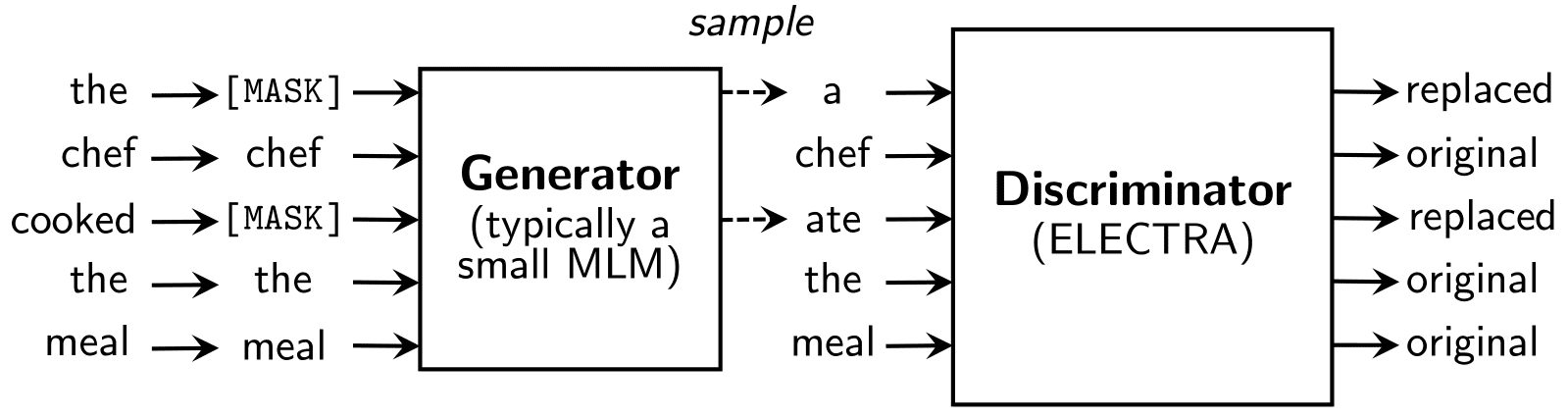
Our approach consists of three steps: (1) self-supervised pre-training on unlabeled natural images (using SimCLR); (2) further self-supervised pre-training using unlabeled medical data (using either SimCLR or MICLe); followed by (3) task-specific supervised fine-tuning using labeled medical data.

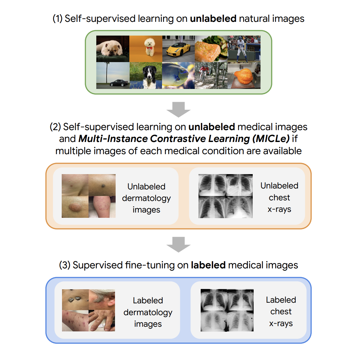
Our approach comprises three steps: (1) Self-supervised pre-training on unlabeled ImageNet using SimCLR (2) Additional self-supervised pre-training using unlabeled medical images. If multiple images of each medical condition are available, a novel Multi-Instance Contrastive Learning (MICLe) strategy is used to construct more informative positive pairs based on different images. (3) Supervised fine-tuning on labeled medical images. Note that unlike step (1), steps (2) and (3) are task and dataset specific.

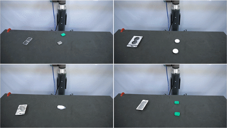
After the initial pre-training with SimCLR on unlabeled natural images is complete, we train the model to capture the special characteristics of medical image datasets. This, too, can be done with SimCLR, but this method constructs positive pairs only through augmentation and does not readily leverage patients' meta data for positive pair construction. Alternatively, we use MICLe, which uses multiple images of the underlying pathology for each patient case, when available, to construct more informative positive pairs for self-supervised learning. Such multi-instance data is often available in medical imaging datasets — e.g., frontal and lateral views of mammograms, retinal fundus images from each eye, etc.

Given multiple images of a given patient case, MICLe constructs a positive pair for self-supervised contrastive learning by drawing two crops from two distinct images from the same patient case. Such images may be taken from different viewing angles and show different body parts with the same underlying pathology. This presents a great opportunity for self-supervised learning algorithms to learn representations that are robust to changes of viewpoint, imaging conditions, and other confounding factors in a direct way. MICLe does not require class label information and only relies on different images of an underlying pathology, the type of which may be unknown.

MICLe generalizes contrastive learning to leverage special characteristics of medical image datasets (patient metadata) to create realistic augmentations, yielding further performance boost of image classifiers.

Combining these self-supervised learning strategies, we show that even in a highly competitive production setting we can achieve a sizable gain of 6.7% in top-1 accuracy on dermatology skin condition classification and an improvement of 1.1% in mean AUC on chest X-ray classification, outperforming strong supervised baselines pre-trained on ImageNet (the prevailing protocol for training medical image analysis models). In addition, we show that self-supervised models are robust to distribution shift and can learn efficiently with only a small number of labeled medical images.

Comparison of Supervised and Self-Supervised Pre-training
Despite its simplicity, we observe that pre-training with MICLe consistently improves the performance of dermatology classification over the original method of pre-training with SimCLR under different pre-training dataset and base network architecture choices. Using MICLe for pre-training, translates to (1.18 ± 0.09)% increase in top-1 accuracy for dermatology classification over using SimCLR. The results demonstrate the benefit accrued from utilizing additional metadata or domain knowledge to construct more semantically meaningful augmentations for contrastive pre-training. In addition, our results suggest that wider and deeper models yield greater performance gains, with ResNet-152 (2x width) models often outperforming ResNet-50 (1x width) models or smaller counterparts.

Comparison of supervised and self-supervised pre-training, followed by supervised fine-tuning using two architectures on dermatology and chest X-ray classification. Self-supervised learning utilizes unlabeled domain-specific medical images and significantly outperforms supervised ImageNet pre-training.

Improved Generalization with Self-Supervised Models
For each task we perform pretraining and fine-tuning using the in-domain unlabeled and labeled data respectively. We also use another dataset obtained in a different clinical setting as a shifted dataset to further evaluate the robustness of our method to out-of-domain data. For the chest X-ray task, we note that self-supervised pre-training with either ImageNet or CheXpert data improves generalization, but stacking them both yields further gains. As expected, we also note that when only using ImageNet for self-supervised pre-training, the model performs worse compared to using only in-domain data for pre-training.

To test the performance under distribution shift, for each task, we held out additional labeled datasets for testing that were collected under different clinical settings. We find that the performance improvement in the distribution-shifted dataset (ChestX-ray14) by using self-supervised pre-training (both using ImageNet and CheXpert data) is more pronounced than the original improvement on the CheXpert dataset. This is a valuable finding, as generalization under distribution shift is of paramount importance to clinical applications. On the dermatology task, we observe similar trends for a separate shifted dataset that was collected in skin cancer clinics and had a higher prevalence of malignant conditions. This demonstrates that the robustness of the self-supervised representations to distribution shifts is consistent across tasks.

Evaluation of models on distribution-shifted datasets for the chest-xray interpretation task. We use the model trained on in-domain data to make predictions on an additional shifted dataset without any further fine-tuning (zero-shot transfer learning). We observe that self-supervised pre-training leads to better representations that are more robust to distribution shifts.

Evaluation of models on distribution-shifted datasets for the dermatology task. Our results generally suggest that self-supervised pre-trained models can generalize better to distribution shifts with MICLe pre-training leading to the most gains.

Improved Label Efficiency
We further investigate the label-efficiency of the self-supervised models for medical image classification by fine-tuning the models on different fractions of labeled training data. We use label fractions ranging from 10% to 90% for both Derm and CheXpert training datasets and examine how the performance varies using the different available label fractions for the dermatology task. First, we observe that pre-training using self-supervised models can compensate for low label efficiency for medical image classification, and across the sampled label fractions, self-supervised models consistently outperform the supervised baseline. These results also suggest that MICLe yields proportionally higher gains when fine-tuning with fewer labeled examples. In fact, MICLe is able to match baselines using only 20% of the training data for ResNet-50 (4x) and 30% of the training data for ResNet152 (2x).

Top-1 accuracy for dermatology condition classification for MICLe, SimCLR, and supervised models under different unlabeled pre-training datasets and varied sizes of label fractions. MICLe is able to match baselines using only 20% of the training data for ResNet-50 (4x).

Conclusion
Supervised pre-training on natural image datasets is commonly used to improve medical image classification. We investigate an alternative strategy based on self-supervised pre-training on unlabeled natural and medical images and find that it can significantly improve upon supervised pre-training, the standard paradigm for training medical image analysis models. This approach can lead to models that are more accurate and label efficient and are robust to distribution shifts. In addition, our proposed Multi-Instance Contrastive Learning method (MICLe) enables the use of additional metadata to create realistic augmentations, yielding further performance boost of image classifiers.

Self-supervised pre-training is much more scalable than supervised pre-training because class label annotation is not required. We hope this paper will help popularize the use of self-supervised approaches in medical image analysis yielding label efficient and robust models suited for clinical deployment at scale in the real world.

Acknowledgements
This work involved collaborative efforts from a multidisciplinary team of researchers, software engineers, clinicians, and cross-functional contributors across Google Health and Google Brain. We thank our co-authors: Basil Mustafa, Fiona Ryan, Zach Beaver, Jan Freyberg, Jon Deaton, Aaron Loh, Alan Karthikesalingam, Simon Kornblith, Ting Chen, Vivek Natarajan, and Mohammad Norouzi. We also thank Yuan Liu from Google Health for valuable feedback and our partners for access to the datasets used in the research.

Source: Google AI Blog

From Vision to Language: Semi-supervised Learning in Action…at Scale

Posted by Thang Luong, Staff Research Scientist, Google Research and Jingcao Hu, Senior Staff Software Engineer, Google Search

Supervised learning, the machine learning task of training predictive models using data points with known outcomes (i.e., labeled data), is generally the preferred approach in industry because of its simplicity. However, supervised learning requires accurately labeled data, the collection of which is often labor intensive. In addition, as model efficiency improves with better architectures, algorithms, and hardware (GPUs / TPUs), training large models to achieve better quality becomes more accessible, which, in turn, requires even more labeled data for continued progress.

To mitigate such data acquisition challenges, semi-supervised learning, a machine learning paradigm that combines a small amount of labeled data with a large amount of unlabeled data, has recently seen success with methods such as UDA, SimCLR, and many others. In our previous work, we demonstrated for the first time that a semi-supervised learning approach, Noisy Student, can achieve state-of-the-art performance on ImageNet, a large-scale academic benchmark for image classification, by utilizing many more unlabeled examples.

Inspired by these results, today we are excited to present semi-supervised distillation (SSD), a simplified version of Noisy Student, and demonstrate its successful application to the language domain. We apply SSD to language understanding within the context of Google Search, resulting in high performance gains. This is the first successful instance of semi-supervised learning applied at such a large scale and demonstrates the potential impact of such approaches for production-scale systems.

Noisy Student Training
Prior to our development of Noisy Student, there was a large body of research into semi-supervised learning. In spite of this extensive research, however, such systems typically worked well only in the low-data regime, e.g., CIFAR, SVHN, and 10% ImageNet. When labeled data were abundant, such models were unable to compete with fully supervised learning systems, which prevented semi-supervised approaches from being applied to important applications in production, such as search engines and self-driving cars. This shortcoming motivated our development of Noisy Student Training, a semi-supervised learning approach that worked well in the high-data regime, and at the time achieved state-of-the-art accuracy on ImageNet using 130M additional unlabeled images.

Noisy Student Training has 4 simple steps:

Train a classifier (the teacher) on labeled data.
The teacher then infers pseudo-labels on a much larger unlabeled dataset.
Then, it trains a larger classifier on the combined labeled and pseudo-labeled data, while also adding noise (noisy student).
(Optional) Going back to step 2, the student may be used as a new teacher.

An illustration of Noisy Student Training through four simple steps. We use two types of noise: model noise (Dropout, Stochastic Depth) and input noise (data augmentation, such as RandAugment).

One can view Noisy Student as a form of self-training, because the model generates pseudo-labels with which it retrains itself to improve performance. A surprising property of Noisy Student Training is that the trained models work extremely well on robustness test sets for which it was not optimized, including ImageNet-A, ImageNet-C, and ImageNet-P. We hypothesize that the noise added during training not only helps with the learning, but also makes the model more robust.

Examples of images that are classified incorrectly by the baseline model, but correctly by Noisy Student. Left: An unmodified image from ImageNet-A. Middle and Right: Images with noise added, selected from ImageNet-C. For more examples including ImageNet-P, please see the paper.

Connections to Knowledge Distillation
Noisy Student is similar to knowledge distillation, which is a process of transferring knowledge from a large model (i.e., the teacher) to a smaller model (the student). The goal of distillation is to improve speed in order to build a model that is fast to run in production without sacrificing much in quality compared to the teacher. The simplest setup for distillation involves a single teacher and uses the same data, but in practice, one can use multiple teachers or a separate dataset for the student.

Simple illustrations of Noisy Student and knowledge distillation.

Unlike Noisy Student, knowledge distillation does not add noise during training (e.g., data augmentation or model regularization) and typically involves a smaller student model. In contrast, one can think of Noisy Student as the process of “knowledge expansion”.

Semi-Supervised Distillation
Another strategy for training production models is to apply Noisy Student training twice: first to get a larger teacher model T’ and then to derive a smaller student S. This approach produces a model that is better than either training with supervised learning or with Noisy Student training alone. Specifically, when applied to the vision domain for a family of EfficientNet models, ranging from EfficientNet-B0 with 5.3M parameters to EfficientNet-B7 with 66M parameters, this strategy achieves much better performance for each given model size (see Table 9 of the Noisy Student paper for more details).

Noisy Student training needs data augmentation, e.g., RandAugment (for vision) or SpecAugment (for speech), to work well. But in certain applications, e.g., natural language processing, such types of input noise are not readily available. For those applications, Noisy Student Training can be simplified to have no noise. In that case, the above two-stage process becomes a simpler method, which we call Semi-Supervised Distillation (SSD). First, the teacher model infers pseudo-labels on the unlabeled dataset from which we then train a new teacher model (T’) that is of equal-or-larger size than the original teacher model. This step, which is essentially self-training, is then followed by knowledge distillation to produce a smaller student model for production.

An illustration of Semi-Supervised Distillation (SSD), a 2-stage process that self-trains an equal-or-larger teacher (T’) before distilling to a student (S).

Improving Search
Having succeeded in the vision domain, an application in the language understanding domain, like Google Search, is a logical next step with broader user impact. In this case, we focus on an important ranking component in Search, which builds on BERT to better understand languages. This task turns out to be well-suited for SSD. Indeed, applying SSD to the ranking component to better understand the relevance of candidate search results to queries achieved one of the highest performance gains among top launches at Search in 2020. Below is an example of a query where the improved model demonstrates better language understanding.

With the implementation of SSD, Search is able to find documents that are more relevant to user queries.

Future Research & Challenges
We have presented a successful instance of semi-supervised distillation (SSD) in the production scale setting of Search. We believe SSD will continue changing the landscape of machine learning usage in the industry from predominantly supervised learning to semi-supervised learning. While our results are promising, there is still much research needed in how to efficiently utilize unlabeled examples in the real world, which is often noisy, and apply them to various domains.

Acknowledgements
Zhenshuai Ding, Yanping Huang, Elizabeth Tucker, Hai Qian, and Steve He contributed immensely to this successful launch. The project would not have succeeded without contributions from members of both the Brain and Search teams: Shuyuan Zhang, Rohan Anil, Zhifeng Chen, Rigel Swavely, Chris Waterson, Avinash Atreya. Thanks to Qizhe Xie and Zihang Dai for feedback on the work. Also, thanks to Quoc Le, Yonghui Wu, Sundeep Tirumalareddy, Alexander Grushetsky, Pandu Nayak for their leadership support.

Source: Google AI Blog

FRILL: On-Device Speech Representations using TensorFlow-Lite

Posted by Joel Shor, Software Engineer, Google Research, Tokyo and Sachin Joglekar, Software Engineer, TensorFlow

Representation learning is a machine learning (ML) method that trains a model to identify salient features that can be applied to a variety of downstream tasks, ranging from natural language processing (e.g., BERT and ALBERT) to image analysis and classification (e.g., Inception layers and SimCLR). Last year, we introduced a benchmark for comparing speech representations and a new, generally-useful speech representation model (TRILL). TRILL is based on temporal proximity, and tries to map speech that occurs close together in time to a lower-dimensional embedding that captures temporal proximity in the embedding space. Since its release, the research community has used TRILL on a diverse set of tasks, such as age classification, video thumbnail selection, and language identification. However, despite achieving state-of-the-art performance, TRILL and other neural network-based approaches require more memory and take longer to compute than signal processing operations that deal with simple features, like loudness, average energy, pitch, etc.

In our recent paper "FRILL: A Non-Semantic Speech Embedding for Mobile Devices", to appear at Interspeech 2021, we create a new model that is 40% the size of TRILL and and a feature set that can be computed over 32x faster on mobile phone, with an average decrease in accuracy of less than 2%. This marks an important step towards fully on-device applications of speech ML models, which will lead to better personalization, improved user experiences and greater privacy, an important aspect of developing AI responsibly. We release the code to create FRILL on github, and a pre-trained FRILL model on TensorFlow Hub.

FRILL: Smaller, Faster TRILL
The TRILL architecture is based on a modified version of ResNet50, an architecture that is computationally taxing for constrained hardware, like mobile phones or smart home devices. On the other hand, architectures like MobileNetV3 have been designed with hardware-aware AutoML to perform well on mobile devices. To take advantage of this, we leverage knowledge distillation to combine the benefits of MobileNetV3’s performance with TRILL’s representations.

In the distillation process, the smaller model (i.e., the "student") tries to match the output of the larger model ("teacher") on the AudioSet dataset. Whereas the original TRILL model learned its weights by optimizing a self-supervised loss that clustered audio segments close in time, the student model learns its weights through a fully-supervised loss that ignores temporal matching and instead tries to match TRILL outputs on the training data. The fully-supervised learning signal is often stronger than self-supervision, and allows us to train more quickly.

Knowledge distillation for non-semantic speech embeddings. The dashed line shows the student model output. The "teacher network" is the TRILL network, where "Layer 19" was the best-performing internal representation. The "Student Hyperparameters" on the left are the options explored in this study, the result of which are 144 distinct models. These models were trained with mean-squared error (MSE) to try to match TRILL's Layer 19.

Choosing the Best Student Model
We perform distillation with a variety of student models, each trained with a specific combination of architecture choices (explained below). To measure each student model’s latency, we leverage TensorFlow Lite (TFLite), a framework that enables execution of TensorFlow models on edge devices. Each candidate model is first converted into TFLite’s flatbuffer format for 32-bit floating point inference and then sent to the target device (in this case, a Pixel 1) for benchmarking. These measurements help us to accurately assess the latency versus quality tradeoffs across all student models and to minimize the loss of quality in the conversion process.

Architecture Choices and Optimizations
We explored different neural network architectures and features that balance latency and accuracy — models with fewer parameters are usually smaller and faster, but have less representational power and therefore generate less generally-useful representations. We trained 144 different models across a number of hyperparameters, all based on the MobileNetV3 architecture:

MobileNetV3 size and width: MobileNetV3 was released in different sizes for use in different environments. The size refers to which MobileNetV3 architecture we used. The width, sometimes known as alpha, proportionally decreases or increases the number of filters in each layer. A width of 1.0 corresponds to the number of filters in the original paper.
Global average pooling: MobileNetV3 normally produces a set of two-dimensional feature maps. These are flattened, concatenated, and passed to the bottleneck layer. However, this bottleneck is often still too large to be computed quickly. We reduce the size of the bottleneck layer kernel by taking the global average of all ”pixels” in each output feature map. Our intuition is that the discarded temporal information is less important for learning a non-semantic speech representation due to the fact that relevant aspects of the signal are stable across time.
Bottleneck compression: A significant portion of the student model’s weights are located in the bottleneck layer. To reduce the size of this layer, we apply a compression operator based on singular value decomposition (SVD) that learns a low-rank approximation of the bottleneck weight matrix.
Quantization-aware training: Since the bottleneck layer has most of the model weights, we use quantization-aware training (QAT) to gradually reduce the numerical precision of the bottleneck weights during training. QAT allows the model to adjust to the lower numerical precision during training, instead of potentially causing performance degradation by introducing quantization after training finishes.

Results
We evaluated each of these models on the Non-Semantic Speech Benchmark (NOSS) and two new tasks — a challenging task to detect whether a speaker is wearing a mask and the human-noise subset of the Environment Sound Classification dataset, which includes labels like “coughing” and “sneezing”. After eliminating models that have strictly better alternatives, we are left with eight ”frontier” models on the quality vs. latency curve, which are the models that had no faster and better performance alternatives at a corresponding quality threshold or latency in our batch of 144 models. We plot the latency vs. quality curve of only these "frontier" models below, and we ignore models that are strictly worse.

Embedding quality and latency tradeoff. The x-axis represents the inference latency and the y-axis shows the difference in accuracy from TRILL’s performance, averaged across benchmark datasets.

FRILL is the best performing sub-10ms inference model, with an inference time of 8.5 ms on a Pixel 1 (about 32x faster than TRILL), and is also roughly 40% the size of TRILL. The frontier curve plateaus at about 10ms latency, which means that at low latency, one can achieve much better performance with minimal latency costs, while achieving improved performance at latencies beyond 10ms is more difficult. This supports our choice of experiment hyperparameters. FRILL's per-task performance is shown in the table below.

	*FRILL*	*TRILL*

Size (MB)	38.5	98.1
Latency (ms)	8.5	275.3

Voxceleb1*	45.5	46.8
Voxforge	78.8	84.5
Speech Commands	81.0	81.7
CREMA-D	71.3	65.9
SAVEE	63.3	70.0
Masked Speech	68.0	65.8
ESC-50 HS	87.9	86.4

Accuracy on each of the classification tasks (higher is better).
*Results in our study use a small subset of Voxceleb1 filtered according to internal privacy guidelines. Interested readers can run our study on the full dataset using TensorFlow Datasets and our open-source evaluation code.

Finally, we evaluate the relative contribution of each of our hyperparameters. We find that for our experiments, quantization-aware training, bottleneck compression and global average pooling most reduced the latency of the resulting models. At the same time bottleneck compression most reduced the quality of the resulting model, while pooling reduced the model performance the least. The architecture width parameter was an important factor in reducing the model size, with minimal performance degradation.

Linear regression weight magnitudes for predicting model quality, latency, and size. The weights indicate the expected impact of changing the input hyperparameter. A higher weight magnitude indicates a greater expected impact.

Our work is an important step in bringing the full benefits of speech machine learning research to mobile devices. We also provide our public model, corresponding model card, and evaluation code to help the research community responsibly develop even more applications for on-device speech representation research.

Acknowledgements
We'd like to thank our paper co-authors: Jacob Peplinksi and Shwetak Patel. We'd like to thank Aren Jansen for his technical support on this project, Françoise Beaufays, and Tulsee Doshi for help open sourcing the model, and Google Research, Tokyo for logistical support.

Source: Google AI Blog

Understanding View Selection for Contrastive Learning

Posted by Yonglong Tian, Student Researcher and Chen Sun, Staff Research Scientist, Google Research

Most people take for granted the ability to view an object from several different angles, but still recognize that it's the same object— a dog viewed from the front is still a dog when viewed from the side. While people do this naturally, computer scientists need to explicitly enable machines to learn representations that are view-invariant, with the goal of seeking robust data representations that retain information that is useful to downstream tasks.

Of course, in order to learn these representations, manually annotated training data can be used. However, as in many cases such annotations aren’t available, which gives rise to a series of self- and crossmodal supervised approaches that do not require manually annotated training data. Currently, a popular paradigm for training with such data is contrastive multiview learning, where two views of the same scene (for example, different image channels, augmentations of the same image, and video and text pairs) will tend to converge in representation space while two views of different scenes diverge. Despite their success, one important question remains: “If one doesn’t have annotated labels readily available, how does one select the views to which the representations should be invariant?” In other words, how does one identify an object using information that resides in the pixels of the image itself, while still remaining accurate when that image is viewed from disparate viewpoints?

In “What makes for good views for contrastive learning”, we use theoretical and empirical analysis to better understand the importance of view selection, and argue that one should reduce the mutual information between views while keeping task-relevant information intact. To verify this hypothesis, we devise unsupervised and semi-supervised frameworks that learn effective views by aiming to reduce their mutual information. We also consider data augmentation as a way to reduce mutual information, and show that increasing data augmentation indeed leads to decreasing mutual information while improving downstream classification accuracy. To encourage further research in this space, we have open-sourced the code and pre-trained models.

The InfoMin Hypothesis
The goal of contrastive multiview learning is to learn a parametric encoder, whose output representations can be used to discriminate between pairs of views with the same identities, and pairs with different identities. The amount and type of information shared between the views determines how well the resulting model performs on downstream tasks. We hypothesize that the views that yield the best results should discard as much information in the input as possible except for the task relevant information (e.g., object labels), which we call the InfoMin principle.

Consider the example below in which two patches of the same image represent the different “views”. The training objective is to identify that the two views belong to the same image. It is undesirable to have views that share too much information, for example, where low-level color and texture cues can be exploited as “shortcuts” (left), or to have views that share too little information to identify that they belong to the same image (right). Rather, views at the “sweet spot” share the information related to downstream tasks, such as patches corresponding to different parts of the panda for an object classification task (center).

An illustration of three regimes of information captured during contrastive multiview learning. Views should not share too much information (left) or too little information (right), but should find an optimal mix (the “sweet spot”, middle) that maximizes the downstream performance.

A Unified View on Contrastive Learning
We design several sets of experiments to verify the InfoMin hypothesis, motivated by the fact that there are simple ways to control the mutual information shared between views without any supervision. For example, we can sample different patches from the same images, and reduce their mutual information simply by increasing the distance between the patches. Here, we estimate the mutual information using InfoNCE (I_NCE), which is a quantitative measure of the mutual information lower bound._. Indeed, we observe a reverse U-shape curve: as mutual information is reduced, the downstream task accuracy first increases and then begins to decrease.

Downstream classification accuracy on STL-10 (left) and CIFAR-10 (right) by applying linear classifiers on representations learned with contrastive learning. Same as the previous illustration, the views are sampled as different patches from the same images. Increasing the Euclidean distance between patches leads to decreasing mutual information. A reverse U-shape curve between classification accuracy and I_NCE (patch distance) is observed.

Furthermore, we demonstrate that several state-of-the-art contrastive learning methods (InstDis, MoCo, CMC, PIRL, SimCLR and CPC) can be unified through the perspective of view selection: despite the differences in architecture, objective and engineering details, all recent contrastive learning methods create two views that implicitly follow the InfoMin hypothesis, where the information shared between views are controlled by the strength of data augmentation. Motivated by this, we propose a new set of data augmentations, which outperforms the prior state of the art, SimCLR, by nearly 4% on the ImageNet linear readout benchmark. We also found that transferring our unsupervised pre-trained models to object detection and instance segmentation consistently outperforms ImageNet pre-training.

Learning to Generate Views
In our work, we design unsupervised and semi-supervised methods that synthesize novel views following the InfoMin hypothesis. We learn flow-based models that transfer natural color spaces into novel color spaces, from which we split the channels to get views. For the unsupervised setup, the view generators are optimized to minimize the InfoNCE bound between views. As shown in the results below, we observe a similar reverse U-shape trend while minimizing the InfoNCE bound.

View generators learned by unsupervised (left) and semi-supervised (right) objectives.

To reach the sweet spot without overly minimizing mutual information, we can use the semi-supervised setup and guide the view generator to retain label information. As expected, all learned views are now centered around the sweet spot, no matter what the input color space is.

Code and Pretrained Models
To accelerate research in self-supervised contastive learning, we are excited to share the code and pretrained models of InfoMin with the academic community. They can be found here.

Acknowledgements
The core team includes Yonglong Tian, Chen Sun, Ben Poole, Dilip Krishnan, Cordelia Schmid and Phillip Isola. We would like to thank Kevin Murphy for insightful discussion; Lucas Beyer for feedback on the manuscript; and the Google Cloud team for computation support.

Source: Google AI Blog

Improving Speech Representations and Personalized Models Using Self-Supervision

Posted by Joel Shor, Software Engineer and Oran Lang, Software Engineer, Google Research, Israel

There are many tasks within speech processing that are easier to solve by having large amounts of data. For example automatic speech recognition (ASR) translates spoken audio into text. In contrast, "non-semantic" tasks focus on the aspects of human speech other than its meaning, encompassing "paralinguistic" tasks, like speech emotion recognition, as well as other kinds of tasks, such as speaker identification, language identification, and certain kinds of voice-based medical diagnoses. In training systems to accomplish these tasks, one common approach is to utilize the largest datasets possible to help ensure good results. However, machine learning techniques that directly rely on massive datasets are often less successful when trained on small datasets.

One way to bridge the performance gap between large and small datasets is to train a representation model on a large dataset, then transfer it to a setting with less data. Representations can improve performance in two ways: they can make it possible to train small models by transforming high-dimensional data (like images and audio) to a lower dimension, and the representation model can also be used as pre-training. In addition, if the representation model is small enough to be run or trained on-device, it can improve performance in a privacy-preserving way by giving users the benefits of a personalized model where the raw data never leaves their device. While representation learning is commonly used in the text domain (e.g. BERT and ALBERT) and in the images domain (e.g. Inception layers and SimCLR), such approaches are underutilized in the speech domain.

Bottom:A large speech dataset is used to train a model, which is then rolled out to other environments. Top Left: On-device personalization — personalized, on-device models combine security and privacy. Top Middle: Small model on embeddings — general-use representations transform high-dimensional, few-example datasets to a lower dimension without sacrificing accuracy; smaller models train faster and are regularized. Top Right: Full model fine-tuning — large datasets can use the embedding model as pre-training to improve performance

Unambiguously improving generally-useful representations, for non-semantic speech tasks in particular, is difficult without a standard benchmark to compare "speech representation usefulness." While the T5 framework systematically evaluates text embeddings and the Visual Task Adaptation Benchmark (VTAB) standardizes image embedding evaluation, both leading to progress in representation learning in those respective fields, there has been no such benchmark for non-semantic speech embeddings.

In "Towards Learning a Universal Non-Semantic Representation of Speech", we make three contributions to representation learning for speech-related applications. First, we present a NOn-Semantic Speech (NOSS) benchmark for comparing speech representations, which includes diverse datasets and benchmark tasks, such as speech emotion recognition, language identification, and speaker identification. These datasets are available in the "audio" section of TensorFlow Datasets. Second, we create and open-source TRIpLet Loss network (TRILL), a new model that is small enough to be executed and fine-tuned on-device, while still outperforming other representations. Third, we perform a large-scale study comparing different representations, and open-source the code used to compute the performance on new representations.

A New Benchmark for Speech Embeddings
For a benchmark to usefully guide model development, it must contain tasks that ought to have similar solutions and exclude those that are significantly different. Previous work either dealt with the variety of possible speech-based tasks independently, or lumped semantic and non-semantic tasks together. Our work improves performance on non-semantic speech tasks, in part, by focusing on neural network architectures that perform well specifically on this subset of speech tasks.

The tasks were selected for the NOSS benchmark on the basis of their 1) diversity — they need to cover a range of use-cases; 2) complexity — they should be challenging; and 3) availability, with particular emphasis on those tasks that are open-source. We combined six datasets of different sizes and tasks.

Datasets for downstream benchmark tasks. *VoxCeleb results in our study were computed using a subset of the dataset that was filtered according to internal policy.

We also introduce three additional intra-speaker tasks to test performance in the personalization scenario. In some datasets with k speakers, we can create k different tasks consisting of training and testing on just a single speaker. Overall performance is averaged across speakers. These three additional intra-speaker tasks measure the ability of an embedding to adapt to a particular speaker, as would be necessary for personalized, on-device models, which are becoming more important as computation moves to smart phones and the internet of things.

To help enable researchers to compare speech embeddings, we’ve added the six datasets in our benchmark to TensorFlow Datasets (in the "audio" section) and open sourced the evaluation framework.

TRILL: A New State of the Art in Non-semantic Speech Classification
Learning an embedding from one dataset and applying it to other tasks is not as common in speech as in other modalities. However, transfer learning, the more general technique of using data from one task to help another (not necessarily with embeddings), has some compelling applications, such as personalizing speech recognizers and voice imitation text-to-speech from few samples. There have been many previously proposed representations of speech, but most of these have been trained on a smaller and less diverse data, have been tested primarily on speech recognition, or both.

To create a data-derived representation of speech that was useful across environments and tasks, we started with AudioSet, a large and diverse dataset that includes about 2500 hours of speech. We then trained an embedding model on a simple, self-supervised criteria derived from previous work on metric learning — embeddings from the same audio should be closer in embedding space than embeddings from different audio. Like BERT and the other text embeddings, the self-supervised loss function doesn't require labels and only relies on the structure of the data itself. This form of self-supervision is the most appropriate for non-semantic speech, since non-semantic phenomena are more stable in time than ASR and other sub-second speech characteristics. This simple, self-supervised criteria captures a large number of acoustic properties that are leveraged in downstream tasks.

TRILL loss: Embeddings from the same audio are closer in embedding space than embeddings from different audio.

TRILL architecture is based on MobileNet, making it fast enough to run on mobile devices. To achieve high accuracy on this small architecture, we distilled the embedding from a larger ResNet50 model without performance degradation.

Benchmark Results
We compared the performance of TRILL against other deep learning representations that are not focused on speech recognition and were trained on similarly diverse datasets. In addition, we compared TRILL to the popular OpenSMILE feature extractor, which uses pre-deep learning techniques (e.g., a fourier transform coefficients, "pitch tracking" using a time-series of pitch measurements, etc.), and randomly initialized networks, which have been shown to be strong baselines. To aggregate the performance across tasks that have different performance characteristics, we first train a small number of simple models, for a given task and embedding. The best result is chosen. Then, to understand the effect that a particular embedding has across all tasks, we calculate a linear regression on the observed accuracies, with both the model and task as the explanatory variables. The effect a model has on the accuracy is the coefficient associated with the model in the regression. For a given task, when changing from one model to another, the resulting change in accuracy is expected to be the difference in y-values in the figure below.

Effect of model on accuracy.

TRILL outperforms the other representations in our study. Factors that contribute to TRILL's success are the diversity of the training dataset, the large context window of the network, and the generality of the TRILL training loss that broadly preserves acoustic characteristics instead of prematurely focusing on certain aspects. Note that representations from intermediate network layers are often more generally useful. The intermediate representations are larger, have finer temporal granularity, and in the case of the classification networks they retain more general information that isn't as specific to the classes on which they were trained.

Another benefit of a generally-useful model is that it can be used to initialize a model on a new task. When the sample size of a new task is small, fine-tuning an existing model may lead to better results than training the model from scratch. We achieved a new state-of-the-art result on three out of six benchmark tasks using this technique, despite doing no dataset-specific hyperparameter tuning.

To compare our new representation, we also tested it on the mask sub-challenge of the Interspeech 2020 Computational Paralinguistics Challenge (ComParE). In this challenge, models must predict whether a speaker is wearing a mask, which would affect their speech. The mask effects are sometimes subtle, and audio clips are only one second long. A linear model on TRILL outperformed the best baseline model, which was a fusion of many models on different kinds of features including traditional spectral and deep-learned features.

Summary
The code to evaluate NOSS is available on GitHub, the datasets are on TensorFlow Datasets, and the TRILL models are available on AI Hub.

The NOn-Semantic Speech benchmark helps researchers create speech embeddings that are useful in a wide range of contexts, including for personalization and small-dataset problems. We provide the TRILL model to the research community as a baseline embedding to surpass.

Acknowledgements
The core team behind this work includes Joel Shor, Aren Jansen, Ronnie Maor, Oran Lang, Omry Tuval, Felix de Chaumont Quitry, Marco Tagliasacchi, Ira Shavitt, Dotan Emanuel, and Yinnon Haviv. We'd also like to thank Avinatan Hassidim and Yossi Matias for technical guidance.

Source: Google AI Blog

Improving Speech Representations and Personalized Models Using Self-Supervision

Datasets for downstream benchmark tasks. *VoxCeleb results in our study were computed using a subset of the dataset that was filtered according to internal policy.

TRILL loss: Embeddings from the same audio are closer in embedding space than embeddings from different audio.

Effect of model on accuracy.

Source: Google AI Blog

Advancing Self-Supervised and Semi-Supervised Learning with SimCLR

Posted by Ting Chen, Research Scientist, and Geoffrey Hinton, VP & Engineering Fellow, Google Research

Recently, natural language processing models, such as BERT and T5, have shown that it is possible to achieve good results with few class labels by first pretraining on a large unlabeled dataset and then fine-tuning on a smaller labeled dataset. Similarly, pretraining on large unlabeled image datasets has the potential to improve performance on computer vision tasks, as demonstrated by Exemplar-CNN, Instance Discrimination, CPC, AMDIM, CMC, MoCo and others. These methods fall under the umbrella of self-supervised learning, which is a family of techniques for converting an unsupervised learning problem into a supervised one by creating surrogate labels from the unlabeled dataset. However, current self-supervised techniques for image data are complex, requiring significant modifications to the architecture or the training procedure, and have not seen widespread adoption.

In “A Simple Framework for Contrastive Learning of Visual Representations”, we outline a method that not only simplifies but also improves previous approaches to self-supervised representation learning on images. Our proposed framework, called SimCLR, significantly advances the state of the art on self- supervised and semi-supervised learning and achieves a new record for image classification with a limited amount of class-labeled data (85.8% top-5 accuracy using 1% of labeled images on the ImageNet dataset). The simplicity of our approach means that it can be easily incorporated into existing supervised learning pipelines. In what follows, we first introduce the SimCLR framework, then discuss three things we discovered while developing SimCLR.

The SimCLR framework
SimCLR first learns generic representations of images on an unlabeled dataset, and then it can be fine-tuned with a small amount of labeled images to achieve good performance for a given classification task. The generic representations are learned by simultaneously maximizing agreement between differently transformed views of the same image and minimizing agreement between transformed views of different images, following a method called contrastive learning. Updating the parameters of a neural network using this contrastive objective causes representations of corresponding views to “attract” each other, while representations of non-corresponding views “repel” each other.

To begin, SimCLR randomly draws examples from the original dataset, transforming each example twice using a combination of simple augmentations (random cropping, random color distortion, and Gaussian blur), creating two sets of corresponding views. The rationale behind these simple transformations of individual images is (1) we want to encourage "consistent" representation of the same image under transformations, (2) since the pretraining data lacks labels, we can’t know a priori which image contains which object class, and 3) we found that these simple transformations are suffice for the neural net to learn good representations, though more sophisticated transformation policy can also be incorporated.

SimCLR then computes the image representation using a convolutional neural network variant based on the ResNet architecture. Afterwards, SimCLR computes a non-linear projection of the image representation using a fully-connected network (i.e., MLP), which amplifies the invariant features and maximizes the ability of the network to identify different transformations of the same image. We use stochastic gradient descent to update both CNN and MLP in order to minimize the loss function of the contrastive objective. After pre-training on the unlabeled images, we can either directly use the output of the CNN as the representation of an image, or we can fine-tune it with labeled images to achieve good performance for downstream tasks.

An illustration of the proposed SimCLR framework. The CNN and MLP layers are trained simultaneously to yield projections that are similar for augmented versions of the same image, while being dissimilar for different images, even if those images are of the same class of object. The trained model not only does well at identifying different transformations of the same image, but also learns representations of similar concepts (e.g., chairs vs. dogs), which later can be associated with labels through fine-tuning.

Performance
Despite its simplicity, SimCLR greatly advances the state of the art in self-supervised and semi-supervised learning on ImageNet. A linear classifier trained on top of self-supervised representations learned by SimCLR achieves 76.5% / 93.2% top-1 / top-5 accuracy, compared to 71.5% / 90.1% from the previous best (CPC v2), matching the performance of supervised learning in a smaller model, ResNet-50, as demonstrated in the following figure.

ImageNet top-1 accuracy of linear classifiers trained on representations learned with different self-supervised methods (pretrained on ImageNet). Gray cross indicates supervised ResNet-50.

When fine-tuned on only 1% of the labels, SimCLR achieves 63.0% / 85.8% top-1 / top-5 accuracy, compared to 52.7% / 77.9% from previous best (CPC v2). Perhaps surprisingly, when fine-tuned on 100% of labels, the pretrained SimCLR models can still significantly outperform supervised baselines trained from scratch, e.g., fine-tuning SimCLR pretrained ResNet-50 (4x) achieves 80.1% top-1 accuracy in 30 epochs, while training it from scratch gets 78.4% in 90 epochs.

Understanding Contrastive Learning of Representations
The improvement SimCLR provides over previous methods is not due to any single design choice, but to their combination. Several important findings are summarized below.

Finding 1: The combinations of image transformations used to generate corresponding views are critical.

As SimCLR learns representations via maximizing agreement of different views of the same image, it is important to compose image transformations to prevent trivial forms of agreement, such as agreement of the color histograms. To understand this better, we explored different types of transformations, illustrated in the figure below.
Random examples of transformations applied to the original image.
We found that while no single transformation (that we studied) suffices to define a prediction task that yields the best representations, two transformations stand out: random cropping and random color distortion. Although neither cropping nor color distortion leads to high performance on its own, composing these two transformations leads to state-of-the-art results.

To understand why combining random cropping with random color distortion is important, consider the process of maximizing agreement between two crops of the same image. This naturally encompasses two types of prediction tasks that enable effective representation learning: (a) predicting local views (e.g., crop A in the image below) from a larger, “global” view (crop B), and (b) predicting neighboring views (e.g., between crop C and crop D).
Maximizing agreement between different crops leads to two prediction tasks. Left: Global vs local views. Right: Adjacent views.
However, different crops of the same image usually look very similar in color space. If the colors are left intact, a model can maximize agreement between crops simply by matching the color histograms. In this case, the model might focus solely on color and ignore other more generalizable features. By independently distorting the colors of each crop, these shallow clues can be removed, and the model can only achieve agreement by learning useful and generalizable representations.
Finding 2: The nonlinear projection is important.

In SimCLR, a MLP-based nonlinear projection is applied before the loss function for contrastive learning objective is calculated, which helps to identify the invariant features of each input image and maximize the ability of the network to identify different transformations of the same image. In our experiments, we found that using such a nonlinear projection helps improve the representation quality, improving the performance of a linear classifier trained on the SimCLR-learned representation by more than 10%.

Interestingly, comparison between the representations used as input for the MLP projection module and the output from the projection reveals that the earlier stage representations perform better when measured by a linear classifier. Since the loss function for contrastive objective is based on the output of the projection, it is somewhat surprising that the representation before the projection is better. We conjecture that our objective leads the final layer of the network to become invariant to features such as color that may be useful for downstream tasks. With the extra nonlinear projection head, the representation layer before the projection head is able to retain more useful information about the image.
Finding 3: Scaling up significantly improves performance.

We found that (1) processing more examples in the same batch, (2) using bigger networks, and (3) training for longer all lead to significant improvements. While these may seem like somewhat obvious observations, these improvements seem larger for SimCLR than for supervised learning. For example, we observe that the performance of a supervised ResNet peaked between 90 and 300 training epochs (on ImageNet), but SimCLR can continue its improvement even after 800 epochs of training. It also seems to be the case when we increase the depth or width of the network — the gain for SimCLR continues, while it starts to saturate for supervised learning. In order to optimize the returns of scaling up our training, we made extensive use of Cloud TPU in our experiments.

Code and Pretrained-Models
To accelerate research in self-supervised and semi-supervised learning, we are excited to share the code and pretrained models of SimCLR with the larger academic community. They can be found on our GitHub repository.

Acknowledgements
This is a joint work with Simon Kornblith and Mohammad Norouzi. We would like to thank Tom Small for the visualization of the SimCLR framework. We are also grateful for general support from Google Research teams in Toronto and elsewhere.

Source: Google AI Blog

More Efficient NLP Model Pre-training with ELECTRA

Posted by Kevin Clark, Student Researcher and Thang Luong, Senior Research Scientist, Google Research, Brain Team

Recent advances in language pre-training have led to substantial gains in the field of natural language processing, with state-of-the-art models such as BERT, RoBERTa, XLNet, ALBERT, and T5, among many others. These methods, though they differ in design, share the same idea of leveraging a large amount of unlabeled text to build a general model of language understanding before being fine-tuned on specific NLP tasks such as sentiment analysis and question answering.

Existing pre-training methods generally fall under two categories: language models (LMs), such as GPT, which process the input text left-to-right, predicting the next word given the previous context, and masked language models (MLMs), such as BERT, RoBERTa, and ALBERT, which instead predict the identities of a small number of words that have been masked out of the input. MLMs have the advantage of being bidirectional instead of unidirectional in that they “see” the text to both the left and right of the token being predicted, instead of only to one side. However, the MLM objective (and related objectives such as XLNet’s) also have a disadvantage. Instead of predicting every single input token, those models only predict a small subset — the 15% that was masked out, reducing the amount learned from each sentence.

Existing pre-training methods and their disadvantages. Arrows indicate which tokens are used to produce a given output representation (rectangle). Left: Traditional language models (e.g., GPT) only use context to the left of the current word. Right: Masked language models (e.g., BERT) use context from both the left and right, but predict only a small subset of words for each input.

In “ELECTRA: Pre-training Text Encoders as Discriminators Rather Than Generators”, we take a different approach to language pre-training that provides the benefits of BERT but learns far more efficiently. ELECTRA — Efficiently Learning an Encoder that Classifies Token Replacements Accurately — is a novel pre-training method that outperforms existing techniques given the same compute budget. For example, ELECTRA matches the performance of RoBERTa and XLNet on the GLUE natural language understanding benchmark when using less than ¼ of their compute and achieves state-of-the-art results on the SQuAD question answering benchmark. ELECTRA’s excellent efficiency means it works well even at small scale — it can be trained in a few days on a single GPU to better accuracy than GPT, a model that uses over 30x more compute. ELECTRA is being released as an open-source model on top of TensorFlow and includes a number of ready-to-use pre-trained language representation models.

Making Pre-training Faster
ELECTRA uses a new pre-training task, called replaced token detection (RTD), that trains a bidirectional model (like a MLM) while learning from all input positions (like a LM). Inspired by generative adversarial networks (GANs), ELECTRA trains the model to distinguish between “real” and “fake” input data. Instead of corrupting the input by replacing tokens with “[MASK]” as in BERT, our approach corrupts the input by replacing some input tokens with incorrect, but somewhat plausible, fakes. For example, in the below figure, the word “cooked” could be replaced with “ate”. While this makes a bit of sense, it doesn’t fit as well with the entire context. The pre-training task requires the model (i.e., the discriminator) to then determine which tokens from the original input have been replaced or kept the same. Crucially, this binary classification task is applied to every input token, instead of only a small number of masked tokens (15% in the case of BERT-style models), making RTD more efficient than MLM — ELECTRA needs to see fewer examples to achieve the same performance because it receives mode training signal per example. At the same time, RTD results in powerful representation learning, because the model must learn an accurate representation of the data distribution in order to solve the task.

Replaced token detection trains a bidirectional model while learning from all input positions.

The replacement tokens come from another neural network called the generator. While the generator can be any model that produces an output distribution over tokens, we use a small masked language model (i.e., a BERT model with small hidden size) that is trained jointly with the discriminator. Although the structure of the generator feeding into the discriminator is similar to a GAN, we train the generator with maximum likelihood to predict masked words, rather than adversarially, due to the difficulty of applying GANs to text. The generator and discriminator share the same input word embeddings. After pre-training, the generator is dropped and the discriminator (the ELECTRA model) is fine-tuned on downstream tasks. Our models all use the transformer neural architecture.

Further details on the replaced token detection (RTD) task. The fake tokens are sampled from a small masked language model that is trained jointly with ELECTRA.

ELECTRA Results
We compare ELECTRA against other state-of-the-art NLP models and found that it substantially improves over previous methods, given the same compute budget, performing comparably to RoBERTa and XLNet while using less than 25% of the compute.

The x-axis shows the amount of compute used to train the model (measured in FLOPs) and the y-axis shows the dev GLUE score. ELECTRA learns much more efficiently than existing pre-trained NLP models. Note that current best models on GLUE such as T5 (11B) do not fit on this plot because they use much more compute than others (around 10x more than RoBERTa).

Further pushing the limits of efficiency, we experimented with a small ELECTRA model that can be trained to good accuracy on a single GPU in 4 days. Although not achieving the same accuracy as larger models that require many TPUs to train, ELECTRA-small still performs quite well, even outperforming GPT while requiring only 1/30th as much compute.

Lastly, to see if the strong results held at scale, we trained a large ELECTRA model using more compute (roughly the same amount as RoBERTa, about 10% the compute as T5). This model achieves a new state-of-the-art for a single model on the SQuAD 2.0 question answering dataset (see the below table) and outperforms RoBERTa, XLNet, and ALBERT on the GLUE leaderboard. While the large-scale T5-11b model scores higher still on GLUE, ELECTRA is 1/30th the size and uses 10% of the compute to train.

*Model*	*Squad 2.0 test set*
ELECTRA-Large	88.7
ALBERT-xxlarge	88.1
XLNet-Large	87.9
RoBERTa-Large	86.8
BERT-Large	80.0

SQuAD 2.0 scores for ELECTRA-Large and other state-of-the-art models (only non-ensemble models shown).

Releasing ELECTRA
We are releasing the code for both pre-training ELECTRA and fine-tuning it on downstream tasks, with currently supported tasks including text classification, question answering and sequence tagging. The code supports quickly training a small ELECTRA model on one GPU. We are also releasing pre-trained weights for ELECTRA-Large, ELECTRA-Base, and ELECTRA-Small. The ELECTRA models are currently English-only, but we hope to release models which have been pre-trained on many languages in the future.

Source: Google AI Blog

SPICE: Self-Supervised Pitch Estimation

Posted by Marco Tagliasacchi, Research Scientist, Google Research

A sound’s pitch is a qualitative measure of its frequency, where a sound with a high pitch is higher in frequency than one of low pitch. Through tracking relative differences in pitch, our auditory system is able to recognize audio features, such as a song’s melody. Pitch estimation has received a great deal of attention over the past decades, due to its central importance in several domains, ranging from music information retrieval to speech analysis.

Traditionally, simple signal processing pipelines were proposed to estimate pitch, working either in the time domain (e.g., pYIN) or in the frequency domain (e.g., SWIPE). But until recently, machine learning methods have not been able to outperform such hand-crafted signal processing pipelines. This was due to the lack of annotated data, which is particularly tedious and difficult to obtain at the temporal and frequency resolution required to train fully supervised models. The CREPE model was able to overcome these limitations to achieve state-of-the-art results by training on a synthetically generated dataset combined with other manually annotated datasets.

In our recent paper, we present a different approach to training pitch estimation models in the absence of annotated data. Inspired by the observation that for humans, including professional musicians, it is typically much easier to estimate relative pitch (the frequency interval between two notes) than absolute pitch (the true fundamental frequency), we designed SPICE (Self-supervised PItCh Estimation) to solve a similar task. This approach relies on self-supervision by defining an auxiliary task (also known as a pretext task) that can be learned in a completely unsupervised way.

Constant-Q transform of an audio clip, superimposed on a representation of pitch as estimated by SPICE (video).

The SPICE model consists of a convolutional encoder, which produces a single scalar embedding that maps linearly to pitch. To accomplish this, we feed two signals to the encoder, a reference signal along with a signal that is pitch shifted from the reference by a random, known amount. Then, we devise a loss function that forces the difference between the scalar embeddings to be proportional to the known difference in pitch. For convenience, we perform pitch shifting in the domain defined by the constant-Q transform (CQT), because this corresponds to a simple translation along the log-spaced frequency axis.

Pitch is well defined only when the underlying signal is harmonic, i.e., when it contains components with integer multiples of the fundamental frequency. So, an important function of the model is to determine when the output is meaningful and reliable. For example, in the figure below, there is no harmonic signal in the interval between 1.2s and 2s resulting in low enough confidence in the pitch estimation that no pitch estimate is generated. SPICE is designed to learn the level of confidence of the pitch estimation in a self-supervised fashion, instead of relying on handcrafted solutions.

SPICE model architecture (simplified). Two pitch-shifted versions of the same CQT frame are fed to two encoders with shared weights. The loss is designed to make the difference between the outputs of the encoders proportional to the relative pitch difference. In addition (not shown), a reconstruction loss is added to regularize the model. The model also learns to produce the confidence of the pitch estimation.

We evaluate our model against publicly available datasets and show that we outperform handcrafted baselines while matching the level of accuracy attained by CREPE, despite having no access to ground truth labels. In addition, by properly augmenting our data during training, SPICE is also able to operate in noisy conditions, e.g., to extract pitch from the singing voice when this is mixed in with background music. The chart below shows a comparison between SWIPE (a hand-crafted signal-processing method), CREPE (a fully supervised model) and SPICE (a self-supervised model) on the MIR-1k dataset.

Evaluation on the MIR-1k dataset, mixing in background music at different signal-to-noise ratios.

The SPICE model has been deployed in FreddieMeter, a web app in which singers can score their performance against Freddie Mercury.

Acknowledgments

The work described here was authored by Beat Gfeller, Christian Frank, Dominik Roblek, Matt Sharifi, Marco Tagliasacchi and Mihajlo Velimirović. We are grateful for all discussions and feedback on this work that we received from our colleagues at Google. The SingingVoices dataset used for training the models in this work has been collected by Alexandra Gherghina as part of FreddieMeter, which is using SPICE and a vocal timbre similarity model to understand how closely a singer matches Freddie Mercury.

Source: Google AI Blog

Learning to Assemble and to Generalize from Self-Supervised Disassembly

Posted by Kevin Zakka, Research Intern and Andy Zeng, Research Scientist, Robotics at Google

Our physical world is full of different shapes, and learning how they are all interconnected is a natural part of interacting with our surroundings — for example, we understand that coat hangers hook onto clothing racks, power plugs insert into wall outlets, and USB cables fit into USB sockets. This general concept of “how things fit together'' based on their shapes is something that people acquire over time and experience, and it helps to increase the efficiency with which we perform tasks, like assembling DIY furniture kits or packing gifts into a box. If robots could learn “how things fit together,” then perhaps they could become more adaptable to new manipulation tasks involving objects they have never seen before, like reconnecting severed pipes, or building makeshift shelters by piecing together debris during disaster response scenarios.

To explore this idea, we worked with researchers from Stanford and Columbia Universities to develop Form2Fit, a robotic manipulation algorithm that uses deep neural networks to learn to visually recognize how objects correspond (or “fit”) to each other. To test this algorithm, we tasked a real robot to perform kit assembly, where it needed to accurately assemble objects into a blister pack or corrugated display to form a single unit. Previous systems built for this task required extensive manual tuning to assemble a single kit unit at a time. However, we demonstrate that by learning the general concept of “how things fit together,” Form2Fit enables our robot to assemble various types of kits with a 94% success rate. Furthermore, Form2Fit is one of the first systems capable of generalizing to new objects and kitting tasks not seen during training.

Form2Fit learns to assemble a wide variety of kits by finding geometric correspondences between object surfaces and their target placement locations. By leveraging geometric information learned from multiple kits during training, the system generalizes to new objects and kits.

While often overlooked, shape analysis plays an important role in manipulation, especially for tasks like kit assembly. In fact, the shape of an object often matches the shape of its corresponding space in the packaging, and understanding this relationship is what allows people to do this task with minimal guesswork. At its core, Form2Fit aims to learn this relationship by training over numerous pairs of objects and their corresponding placing locations across multiple different kitting tasks – with the goal to acquire a broader understanding of how shapes and surfaces fit together. Form2Fit improves itself over time with minimal human supervision, gathering its own training data by repeatedly disassembling completed kits through trial and error, then time-reversing the disassembly sequences to get assembly trajectories. After training overnight for 12 hours, our robot learns effective pick and place policies for a variety of kits, achieving 94% assembly success rates with objects and kits in varying configurations, and over 86% assembly success rates when handling completely new objects and kits.

Data-Driven Shape Descriptors For Generalizable Assembly
The core component of Form2Fit is a two-stream matching network that learns to infer orientation-sensitive geometric pixel-wise descriptors for objects and their target placement locations from visual data. These descriptors can be understood as compressed 3D point representations that encode object geometry, textures, and contextual task-level knowledge. Form2Fit uses these descriptors to establish correspondences between objects and their target locations (i.e., where they should be placed). Since these descriptors are orientation-sensitive, they allow Form2Fit to infer how the picked object should be rotated before it is placed in its target location.

Form2Fit uses two additional networks to generate valid pick and place candidates. A suction network gets fed a 3D image of the objects and generates pixel-wise predictions of suction success. The suction probability map is visualized as a heatmap, where hotter pixels indicate better locations to grasp the object at the 3D location of the corresponding pixel. In parallel, a place network gets fed a 3D image of the target kit and outputs pixel-wise predictions of placement success. These, too, are visualized as a heatmap, where higher confidence values serve as better locations for the robot arm to approach from a top-down angle to place the object. Finally, the planner integrates the output of all three modules to produce the final pick location, place location and rotation angle.

Overview of Form2Fit. The suction and place networks infer candidate picking and placing locations in the scene respectively. The matching network generates pixel-wise orientation-sensitive descriptors to match picking locations to their corresponding placing locations. The planner then integrates it all to control the robot to execute the next best pick and place action.

Learning Assembly from Disassembly
Neural networks require large amounts of training data, which can be difficult to collect for tasks like assembly. Precisely inserting objects into tight spaces with the correct orientation (e.g., in kits) is challenging to learn through trial and error, because the chances of success from random exploration can be slim. In contrast, disassembling completed units is often easier to learn through trial and error, since there are fewer incorrect ways to remove an object than there are to correctly insert it. We leveraged this difference in order to amass training data for Form2Fit.

An example of self-supervision through time-reversal: rewinding a disassembly sequence of a deodorant kit over time generates a valid assembly sequence.

Our key observation is that in many cases of kit assembly, a disassembly sequence – when reversed over time – becomes a valid assembly sequence. This concept, called time-reversed disassembly, enables Form2Fit to train entirely through self-supervision by randomly picking with trial and error to disassemble a fully-assembled kit, then reversing that disassembly sequence to learn how the kit should be put together.

Generalization Results
The results of our experiments show great potential for learning generalizable policies for assembly. For instance, when a policy is trained to assemble a kit in only one specific position and orientation, it can still robustly assemble random rotations and translations of the kit 90% of the time.

Form2Fit policies are robust to a wide range of rotations and translations of the kits.

We also find that Form2Fit is capable of tackling novel configurations it has not been exposed to during training. For example, when training a policy on two single-object kits (floss and tape), we find that it can successfully assemble new combinations and mixtures of those kits, even though it has never seen such configurations before.

Form2Fit policies can generalize to novel kit configurations such as multiple versions of the same kit and mixtures of different kits.

Furthermore, when given completely novel kits on which it has not been trained, Form2Fit can generalize using its learned shape priors to assemble those kits with over 86% assembly accuracy.

Form2Fit policies can generalize to never-before-seen single and multi-object kits.

What Have the Descriptors Learned?
To explore what the descriptors of the matching network from Form2Fit have learned to encode, we visualize the pixel-wise descriptors of various objects in RGB colorspace through use of an embedding technique called t-SNE.

The t-SNE embedding of the learned object descriptors. Similarly oriented objects of the same category display identical colors (e.g. A, B or F, G) while different objects (e.g. C, H) and same objects but different orientation (e.g. A, C, D or H, F) exhibit different colors.

We observe that the descriptors have learned to encode (a) rotation — objects oriented differently have different descriptors (A, C, D, E) and (H, F); (b) spatial correspondence — same points on the same oriented objects share similar descriptors (A, B) and (F, G); and (c) object identity — zoo animals and fruits exhibit unique descriptors (columns 3 and 4).

Limitations & Future Work
While Form2Fit’s results are promising, its limitations suggest directions for future work. In our experiments, we assume a 2D planar workspace to constrain the kit assembly task so that it can be solved by sequencing top-down picking and placing actions. This may not work for all cases of assembly – for example, when a peg needs to be precisely inserted at a 45 degree angle. It would be interesting to expand Form2Fit to more complex action representations for 3D assembly.

You can learn more about this work and download the code from our GitHub repository.

Acknowledgments
This research was done by Kevin Zakka, Andy Zeng, Johnny Lee, and Shuran Song (faculty at Columbia University), with special thanks to Nick Hynes, Alex Nichol, and Ivan Krasin for fruitful technical discussions; Adrian Wong, Brandon Hurd, Julian Salazar, and Sean Snyder for hardware support; Ryan Hickman for valuable managerial support; and Chad Richards for helpful feedback on writing.

googblogs.com

All Google blogs and Press in one site

Tag Archives: Self-Supervised Learning

Self-Supervised Learning Advances Medical Image Classification

Source: Google AI Blog

From Vision to Language: Semi-supervised Learning in Action…at Scale

Source: Google AI Blog

FRILL: On-Device Speech Representations using TensorFlow-Lite

Source: Google AI Blog

Understanding View Selection for Contrastive Learning

Source: Google AI Blog

Improving Speech Representations and Personalized Models Using Self-Supervision

Source: Google AI Blog

Improving Speech Representations and Personalized Models Using Self-Supervision

Source: Google AI Blog

Advancing Self-Supervised and Semi-Supervised Learning with SimCLR

Source: Google AI Blog

More Efficient NLP Model Pre-training with ELECTRA

Source: Google AI Blog

SPICE: Self-Supervised Pitch Estimation

Source: Google AI Blog

Learning to Assemble and to Generalize from Self-Supervised Disassembly

Source: Google AI Blog