Tag Archives: reinforcement learning

Quickly Training Game-Playing Agents with Machine Learning

In the last two decades, dramatic advances in compute and connectivity have allowed game developers to create works of ever-increasing scope and complexity. Simple linear levels have evolved into photorealistic open worlds, procedural algorithms have enabled games with unprecedented variety, and expanding internet access has transformed games into dynamic online services. Unfortunately, scope and complexity have grown more rapidly than the size of quality assurance teams or the capabilities of traditional automated testing. This poses a challenge to both product quality (such as delayed releases and post-launch patches) and developer quality of life.

Machine learning (ML) techniques offer a possible solution, as they have demonstrated the potential to profoundly impact game development flows – they can help designers balance their game and empower artists to produce high-quality assets in a fraction of the time traditionally required. Furthermore, they can be used to train challenging opponents that can compete at the highest levels of play. Yet some ML techniques can pose requirements that currently make them impractical for production game teams, including the design of game-specific network architectures, the development of expertise in implementing ML algorithms, or the generation of billions of frames of training data. Conversely, game developers operate in a setting that offers unique advantages to leverage ML techniques, such as direct access to the game source, an abundance of expert demonstrations, and the uniquely interactive nature of video games.

Today, we present a ML-based system that game developers can use to quickly and efficiently train game-testing agents, helping developers find serious bugs quickly while allowing human testers to focus on more complex and intricate problems. The resulting solution requires no ML expertise, works on many of the most popular game genres, and can train an ML policy, which generates game actions from game state, in less than an hour on a single game instance. We have also released an open source library that demonstrates a functional application of these techniques.

Supported genres include arcade, action/adventure, and racing games.

The Right Tool for the Right Job
The most elemental form of video game testing is to simply play the game. A lot. Many of the most serious bugs (such as crashes or falling out of the world) are easy to detect and fix; the challenge is finding them within the vast state space of a modern game. As such, we decided to focus on training a system that could “just play the game” at scale.

We found that the most effective way to do this was not to try to train a single, super effective agent that could play the entire game from end-to-end, but to provide developers with the ability to train an ensemble of game-testing agents, each of which could effectively accomplish tasks of a few minutes each, which game developers refer to as “gameplay loops”.

These core gameplay behaviors are often expensive to program through traditional means, but are much more efficient to train than a single end-to-end ML model. In practice, commercial games create longer loops by repeating and remixing core gameplay loops, which means that developers can test large stretches of gameplay by combining ML policies with a small amount of simple scripting.

Simulation-centric, Semantic API
One of the most fundamental challenges in applying ML to game development is bridging the chasm between the simulation-centric world of video games and the data-centric world of ML. Rather than ask developers to directly convert the game state into custom, low-level ML features (which would be too labor intensive) or attempting to learn from raw pixels (which would require too much data to train), our system provides developers with an idiomatic, game-developer friendly API that allows them to describe their game in terms of the essential state that a player observes and the semantic actions they can perform. All of this information is expressed via concepts that are familiar to game developers, such as entities, raycasts, 3D positions and rotations, buttons and joysticks.

As you can see in the example below, the API allows the specification of observations and actions in just a few lines of code.
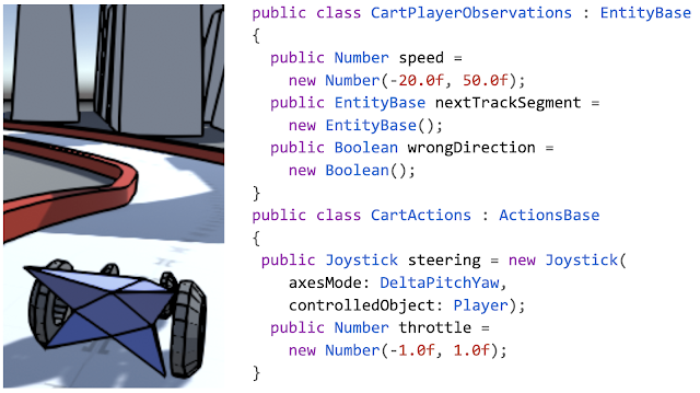
Example actions and observations for a racing game.

From API to Neural Network
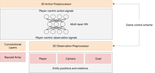
This high level, semantic API is not just easy to use but also allows the system to flexibly adapt to the specific game being developed – the specific combination of API building blocks employed by the game developer informs our choice of network architecture, since it provides information about the type of gaming scenario in which the system is deployed. Some examples of this include: handling action outputs differently depending on whether they represent a digital button or analog joystick, or using techniques from image processing to handle observations that result from an agent probing its environment with raycasts (similar to how autonomous vehicles probe their environment with LIDAR).

Our API is sufficiently general to allow modeling of many common control-schemes (the configuration of action outputs that control movement) in games, such as first-person games, third-person games with camera-relative controls, racing games, twin stick shooters, etc. Since 3D movement and aiming are often an integral aspect of gameplay in general, we create networks that automatically tend towards simple behaviors such as aiming, approach or avoidance in these games. The system accomplishes this by analyzing the game’s control scheme to create neural network layers that perform custom processing of observations and actions in that game. For example, positions and rotations of objects in the world are automatically translated into directions and distances from the point of view of the AI-controlled game entity. This transformation typically increases the speed of learning and helps the learned network generalize better.

An example neural network generated for a game with joystick controls and raycast inputs. Depending on the inputs (red) and the control scheme, the system generates custom pre- and post-processing layers (orange).

Learning From The Experts in Real Time
After generating a neural network architecture, the network needs to be trained to play the game using an appropriate choice of learning algorithm.

Reinforcement learning (RL), in which an ML policy is trained directly to maximize a reward, may seem like the obvious choice since they have been successfully used to train highly competent ML policies for games. However, RL algorithms tend to require more data than a single game instance can produce in a reasonable amount of time, and achieving good results in a new domain often requires hyperparameter tuning and strong ML domain knowledge.

Instead, we found that imitation learning (IL), which trains ML policies based by observing experts play the game, works well for our use case. Unlike RL, where the agent needs to discover a good policy on its own, IL only needs to recreate the behavior of a human expert. Since game developers and testers are experts in their own games, they can easily provide demonstrations of how to play the game.

We use an IL approach inspired by the DAgger algorithm, which allows us to take advantage of video games’ most compelling quality – interactivity. Thanks to the reductions in training time and data requirements enabled by our semantic API, training is effectively realtime, giving a developer the ability to fluidly switch between providing gameplay demonstrations and watching the system play. This results in a natural feedback loop, in which a developer iteratively provides corrections to a continuous stream of ML policies.

From the developer’s perspective, providing a demonstration or a correction to faulty behavior is as simple as picking up the controller and starting to play the game. Once they are done, they can put the controller down and watch the ML policy play. The result is a training experience that is real-time, interactive, highly experiential, and, very often, more than a little fun.
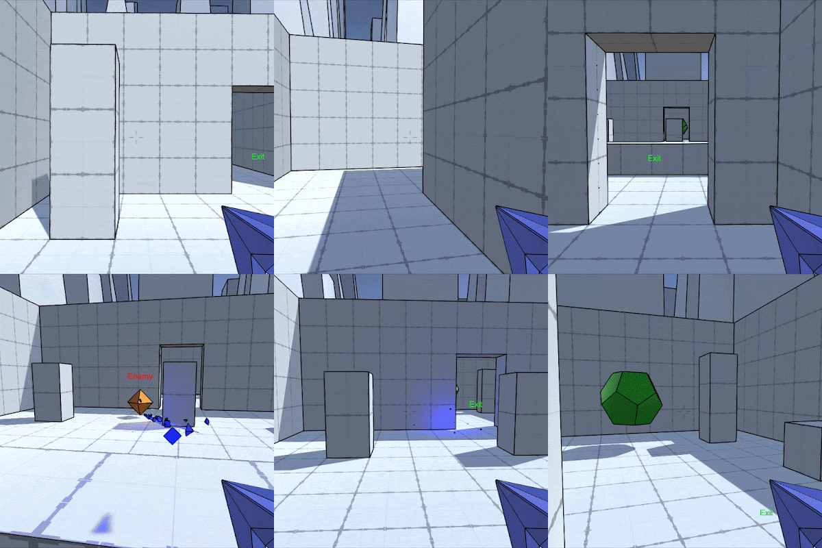
ML policy for an FPS game, trained with our system.

Conclusion
We present a system which combines a high-level semantic API with a DAgger-inspired interactive training flow that enables training of useful ML policies for video game testing in a wide variety of genres. We have released an open source library as a functional illustration of our system. No ML expertise is required and training of agents for test applications often takes less than an hour on a single developer machine. We hope that this work will help inspire the development of ML techniques that can be deployed in real-world game-development flows in ways that are accessible, effective, and fun to use.

Acknowledgements
We’d like to thank the core members of the project: Dexter Allen, Leopold Haller, Nathan Martz, Hernan Moraldo, Stewart Miles and Hina Sakazaki. Training algorithms are provided by TF Agents, and on-device inference by TF Lite. Special thanks to our research advisors, Olivier Bachem, Erik Frey, and Toby Pohlen, and to Eugene Brevdo, Jared Duke, Oscar Ramirez and Neal Wu who provided helpful guidance and support.
Source: Google AI Blog


Flexible, Scalable, Differentiable Simulation of Recommender Systems with RecSim NG

Recommender systems are the primary interface connecting users to a wide variety of online content, and therefore must overcome a number of challenges across the user population in order to serve them equitably. To this end, in 2019 we released RecSim, a configurable platform for authoring simulation environments to facilitate the study of RL algorithms (the de facto standard ML approach for addressing sequential decision problems) in recommender systems. However, as the technology has progressed, it has become increasingly important to address the gap between simulation and real-world applications, ensuring that models are flexible and easily extendible, enabling probabilistic inference of user dynamics, and addressing computational efficiency.

To address these issues, we recently released RecSim NG, the “Next Generation” of simulators for recommender systems research and development. RecSim NG is a response to a set of use cases that have emerged as important challenges in the application of simulation to real-world problems. It addresses the gap between simulation and real-world applications, ensures the models are flexible and easily extendible, enables probabilistic inference of user dynamics, and addresses computational efficiency.

Overview of RecSim NG
RecSim NG is a scalable, modular, differentiable simulator implemented in Edward2 and TensorFlow. It offers a powerful, general probabilistic programming language for agent-behavior specification.

RecSim NG significantly expands the modeling capabilities of RecSim in two ways. First, the story API allows the simulation of scenarios where an arbitrary number of actors (e.g., recommenders, content consumers, content producers, advertisers) interact with one another. This enables the flexible modeling of entire recommender ecosystems, as opposed to the usual isolated user-recommender interaction setting. Second, we introduced a library of behavioral building blocks that, much like Keras layers, implement well-known modeling primitives that can be assembled to build complex models quickly. Following the object-oriented paradigm, RecSim NG uses entity patterns to encapsulate shared parameters that govern various agent behaviors, like user satisfaction, and uses templates to define large populations of agents concisely in a way that abstracts agent “individuality” without duplicating invariant behaviors.

Apart from the typical use of simulators to generate Monte Carlo samples, RecSim NG directly enables various other forms of probabilistic reasoning. While domain knowledge and intuition are key to modeling any recommendation problem, the simulation fidelity needed to bridge the so-called “sim2real” gap can only be achieved by calibrating the simulator’s model to observed data. For data-driven simulation, RecSim NG makes it easy to implement various model-learning algorithms, such as expectation-maximization (EM), generative adversarial training, etc.

Also available within RecSim NG are tools for probabilistic inference and latent-variable model learning, backed by automatic differentiation and tracing. RecSim NG exposes a small set of Edward2 program transformations tailored to simulation-specific tasks. Its log-probability module can evaluate the probabilities of trajectories according to the probabilistic graphical model induced by the simulation. This, together with the automatic differentiation provided by the TensorFlow runtime, enables the implementation of maximum-likelihood estimation and model learning within the simulation itself. RecSim NG can readily use the Markov-chain Monte Carlo (MCMC) machinery provided by TensorFlow Probability to power posterior inference and latent-variable model learning. For example, a simulation model that describes how latent user attributes (e.g., preferences, intents, satisfaction) are translated into observational data (e.g., clicks, ratings, comments) can be “run in reverse,” that is, real observational data generated by a recommender system can be used to identify the most likely configuration of latent user attributes, which in turn can be used to assess the quality of the user experience. This allows for a simulation model to be integrated directly into the full data-science and model-development workflow.

Assessing recommender ecosystem health, i.e., the long-term impact of recommendation strategies on aspects such as overall satisfaction, collective fairness, and safety, requires the simulation of large multi-agent systems in order to plausibly reproduce the interactions between the different participants of the ecosystem. This, along with the computational load of probabilistic inference tasks, requires an efficient simulation runtime. For computational performance, RecSim NG offers a TensorFlow-based runtime for running simulations on accelerated hardware. The simulation takes advantage of all optimizations offered by TensorFlow's AutoGraph compiler, including accelerated linear algebra (XLA) if available. The simulation will automatically exploit all available cores on the host machine as well as specialized hardware (if run accordingly), such as Tensor Processing Units (TPUs). The core RecSim NG architecture is back-end independent, enabling applications to be developed within other computational frameworks (such as JAX or PyTorch).

Ecosystem Modeling as an Application
To demonstrate the capabilities of RecSim NG, we present a very simplified model of multi-agent interactions among users and content providers in a stylized recommender ecosystem1. The simulation captures the dynamics of a recommender system that mediates the interaction between users and content providers by recommending slates of those providers’ content items to users over time. We adopt a simplified user model whereby each user is characterized by a static, observable “user interest vector.” This vector determines a user’s affinity with a recommended item, which are then used as inputs to a choice model that determines a user’s item selection from a recommended slate. A user’s utility for any selected item is simply their affinity for the item, perturbed with Gaussian noise.

The aim of the recommender is to maximize cumulative user utility, over all users, over a fixed horizon. However, interesting ecosystem effects make this challenging, and emerge because of content provider behavior. Like users, each provider has an “interest vector'' around which the content items it makes available are centered, reflecting that provider’s general expertise or tendencies. Providers have their own incentives for making content available: their utility is measured by the number of their items selected by any user over the recent past. Moreover, providers with higher utility generate or make available a greater number of items, increasing the “catalog” from which users (and the recommender) can choose.

We compare two different recommender policies in this setting. The first is a standard “myopic'' policy that, for any user, always recommends the items that have the greatest predicted affinity for that user. Under such a policy, the behavior of providers has the potential to give rise to “rich-get-richer'' phenomena: providers that initially attract users produce more items at subsequent periods, which increases the odds of attracting even further future engagement. This gradual concentration of available items around “mainstream” content providers has a negative impact on overall user utility over time. The second recommender policy is aware of these provider dynamics, which it counteracts by promoting under-served providers.2 While a simple heuristic, the provider-aware policy increases overall user utility over extended horizons.

The number of agents in the simulation is large and we templatize both users and content providers with reusable modeling blocks offered by RecSim NG. Determining how to execute the simulation in parallel is non-trivial, so it is critical to utilize TF's AutoGraph and other computational optimizations.

Conclusion
Our hope is that RecSim NG will make it easier for both researchers and practitioners to develop, train and evaluate novel algorithms for recommender systems, especially algorithms intended to optimize system behavior over extended horizons, capture complex multi-agent interactions and incentives, or both. We are also investigating the release of increasingly realistic user models that can serve as benchmarks for the research community, as well as methods that can facilitate “sim2real” transfer using RecSim NG.

Further details regarding the RecSim NG framework can be found in the associated white paper, while code and colabs/tutorials are available here. A video about RecSim NG presented at RecSys-2020 is shown below:

Acknowledgements
We thank our collaborators and early adopters of RᴇᴄSɪᴍ NG, including the other members of the RecSim NG team: Vihan Jain, Eugene Ie, Chris Colby, Nicolas Mayoraz, Hubert Pham, Dustin Tran, Ivan Vendrov and Craig Boutilier.


1 This model is a much simpler version of that presented in this ICML-20 paper

2 This simple heuristic policy is used only to demonstrate RecSim NG’s capabilities. More sophisticated algorithms that compute policies that explicitly maximize long-term user utility are discussed in this ICML-20 paper

Source: Google AI Blog


Evolving Reinforcement Learning Algorithms

A long-term, overarching goal of research into reinforcement learning (RL) is to design a single general purpose learning algorithm that can solve a wide array of problems. However, because the RL algorithm taxonomy is quite large, and designing new RL algorithms requires extensive tuning and validation, this goal is a daunting one. A possible solution would be to devise a meta-learning method that could design new RL algorithms that generalize to a wide variety of tasks automatically.

In recent years, AutoML has shown great success in automating the design of machine learning components, such as neural networks architectures and model update rules. One example is Neural Architecture Search (NAS), which has been used to develop better neural network architectures for image classification and efficient architectures for running on phones and hardware accelerators. In addition to NAS, AutoML-Zero shows that it’s even possible to learn the entire algorithm from scratch using basic mathematical operations. One common theme in these approaches is that the neural network architecture or the entire algorithm is represented by a graph, and a separate algorithm is used to optimize the graph for certain objectives.

These earlier approaches were designed for supervised learning, in which the overall algorithm is more straightforward. But in RL, there are more components of the algorithm that could be potential targets for design automation (e.g., neural network architectures for agent networks, strategies for sampling from the replay buffer, overall formulation of the loss function), and it is not always clear what the best model update procedure would be to integrate these components. Prior efforts for the automation RL algorithm discovery have focused primarily on model update rules. These approaches learn the optimizer or RL update procedure itself and commonly represent the update rule with a neural network such as an RNN or CNN, which can be efficiently optimized with gradient-based methods. However, these learned rules are not interpretable or generalizable, because the learned weights are opaque and domain specific.

In our paper “Evolving Reinforcement Learning Algorithms”, accepted at ICLR 2021, we show that it’s possible to learn new, analytically interpretable and generalizable RL algorithms by using a graph representation and applying optimization techniques from the AutoML community. In particular, we represent the loss function, which is used to optimize an agent’s parameters over its experience, as a computational graph, and use Regularized Evolution to evolve a population of the computational graphs over a set of simple training environments. This results in increasingly better RL algorithms, and the discovered algorithms generalize to more complex environments, even those with visual observations like Atari games.

RL Algorithm as a Computational Graph
Inspired by ideas from NAS, which searches over the space of graphs representing neural network architectures, we meta-learn RL algorithms by representing the loss function of an RL algorithm as a computational graph. In this case, we use a directed acyclic graph for the loss function, with nodes representing inputs, operators, parameters and outputs. For example, in the computational graph for DQN, input nodes include data from the replay buffer, operator nodes include neural network operators and basic math operators, and the output node represents the loss, which will be minimized with gradient descent.

There are a few benefits of such a representation. This representation is expressive enough to define existing algorithms but also new, undiscovered algorithms. It is also interpretable. This graph representation can be analyzed in the same way as human designed RL algorithms, making it more interpretable than approaches that use black box function approximators for the entire RL update procedure. If researchers can understand why a learned algorithm is better, then they can both modify the internal components of the algorithm to improve it and transfer the beneficial components to other problems. Finally, the representation supports general algorithms that can solve a wide variety of problems.

Example computation graph for DQN which computes the squared Bellman error.

We implemented this representation using the PyGlove library, which conveniently turns the graph into a search space that can be optimized with regularized evolution.

Evolving RL Algorithms
We use an evolutionary based approach to optimize the RL algorithms of interest. First, we initialize a population of training agents with randomized graphs. This population of agents is trained in parallel over a set of training environments. The agents first train on a hurdle environment — an easy environment, such as CartPole, intended to quickly weed out poorly performing programs.

If an agent cannot solve the hurdle environment, the training is stopped early with a score of zero. Otherwise the training proceeds to more difficult environments (e.g., Lunar Lander, simple MiniGrid environments, etc.). The algorithm performance is evaluated and used to update the population, where more promising algorithms are further mutated. To reduce the search space, we use a functional equivalence checker which will skip over newly proposed algorithms if they are functionally the same as previously examined algorithms. This loop continues as new mutated candidate algorithms are trained and evaluated. At the end of training, we select the best algorithm and evaluate its performance over a set of unseen test environments.

The population size in the experiments was around 300 agents, and we observed the evolution of good candidate loss functions after 20-50 thousand mutations, requiring about three days of training. We were able to train on CPUs because the training environments were simple, controlling for the computational and energy cost of training. To further control the cost of training, we seeded the initial population with human-designed RL algorithms such as DQN.

Overview of meta-learning method. Newly proposed algorithms must first perform well on a hurdle environment before being trained on a set of harder environments. Algorithm performance is used to update a population where better performing algorithms are further mutated into new algorithms. At the end of training, the best performing algorithm is evaluated on test environments.

Learned Algorithms
We highlight two discovered algorithms that exhibit good generalization performance. The first is DQNReg, which builds on DQN by adding a weighted penalty on the Q-values to the normal squared Bellman error. The second learned loss function, DQNClipped, is more complex, although its dominating term has a simple form — the max of the Q-value and the squared Bellman error (modulo a constant). Both algorithms can be viewed as a way to regularize the Q-values. While DQNReg adds a soft constraint, DQNClipped can be interpreted as a kind of constrained optimization that will minimize the Q-values if they become too large. We show that this learned constraint kicks in during the early stage of training when overestimating the Q-values is a potential issue. Once this constraint is satisfied, the loss will instead minimize the original squared Bellman error.

A closer analysis shows that while baselines like DQN commonly overestimate Q-values, our learned algorithms address this issue in different ways. DQNReg underestimates the Q-values, while DQNClipped has similar behavior to double dqn in that it slowly approaches the ground truth without overestimating it.

It’s worth pointing out that these two algorithms consistently emerge when the evolution is seeded with DQN. Learning from scratch, the method rediscovers the TD algorithm. For completeness, we release a dataset of top 1000 performing algorithms discovered during evolution. Curious readers could further investigate the properties of these learned loss functions.

Overestimated values are generally a problem in value-based RL. Our method learns algorithms that have found a way to regularize the Q-values and thus reduce overestimation.

Learned Algorithms Generalization Performance
Normally in RL, generalization refers to a trained policy generalizing across tasks. However, in this work we’re interested in algorithmic generalization performance, which means how well an algorithm works over a set of environments. On a set of classical control environments, the learned algorithms can match baselines on the dense reward tasks (CartPole, Acrobot, LunarLander) and outperform DQN on the sparser reward task, MountainCar.

Performance of learned algorithms versus baselines on classical control environments.

On a set of sparse reward MiniGrid environments, which test a variety of different tasks, we see that DQNReg greatly outperforms baselines on both the training and test environments, in terms of sample efficiency and final performance. In fact, the effect is even more pronounced on the test environments, which vary in size, configuration, and existence of new obstacles, such as lava.

Training environment performance versus training steps as measured by episode return over 10 training seeds. DQNReg can match or outperform baselines in sample efficiency and final performance.
DQNReg can greatly outperform baselines on unseen test environments.

We visualize the performance of normal DDQN vs. the learned algorithm DQNReg on a few MiniGrid environments. The starting location, wall configuration, and object configuration of these environments are randomized at each reset, which requires the agent to generalize instead of simply memorizing the environment. While DDQN often struggles to learn any meaningful behavior, DQNReg can learn the optimal behavior efficiently.

DDQN
DQNReg (Learned) 

Even on image-based Atari environments we observe improved performance, even though training was on non-image-based environments. This suggests that meta-training on a set of cheap but diverse training environments with a generalizable algorithm representation could enable radical algorithmic generalization.

EnvDQNDDQNPPODQNReg
Asteroid1364.5734.72097.52390.4
Bowling50.468.140.180.5
Boxing88.091.694.6100.0
RoadRunner  39544.0    44127.0    35466.0    65516.0  
Performance of learned algorithm, DQNReg, against baselines on several Atari games. Performance is evaluated over 200 test episodes every 1 million steps.

Conclusion
In this post, we’ve discussed learning new interpretable RL algorithms by representing their loss functions as computational graphs and evolving a population of agents over this representation. The computational graph formulation allows researchers to both build upon human-designed algorithms and study the learned algorithms using the same mathematical toolset as the existing algorithms. We analyzed a few of the learned algorithms and can interpret them as a form of entropy regularization to prevent value overestimation. These learned algorithms can outperform baselines and generalize to unseen environments. The top performing algorithms are available for further analytical study.

We hope that future work will extend to more varied RL settings such as actor critic algorithms or offline RL. Furthermore we hope that this work can lead to machine assisted algorithm development where computational meta-learning can help researchers find new directions to pursue and incorporate learned algorithms into their own work.

Acknowledgements
We thank our co-authors Daiyi Peng, Esteban Real, Sergey Levine, Quoc V. Le, Honglak Lee, and Aleksandra Faust. We also thank Luke Metz for helpful early discussions and feedback on the paper, Hanjun Dai for early discussions on related research ideas, Xingyou Song, Krzysztof Choromanski, and Kevin Wu for helping with infrastructure, and Jongwook Choi for helping with environment selection. Finally we thank Tom Small for designing animations for this post.

Source: Google AI Blog


Multi-Task Robotic Reinforcement Learning at Scale

For general-purpose robots to be most useful, they would need to be able to perform a range of tasks, such as cleaning, maintenance and delivery. But training even a single task (e.g., grasping) using offline reinforcement learning (RL), a trial and error learning method where the agent uses training previously collected data, can take thousands of robot-hours, in addition to the significant engineering needed to enable autonomous operation of a large-scale robotic system. Thus, the computational costs of building general-purpose everyday robots using current robot learning methods becomes prohibitive as the number of tasks grows.

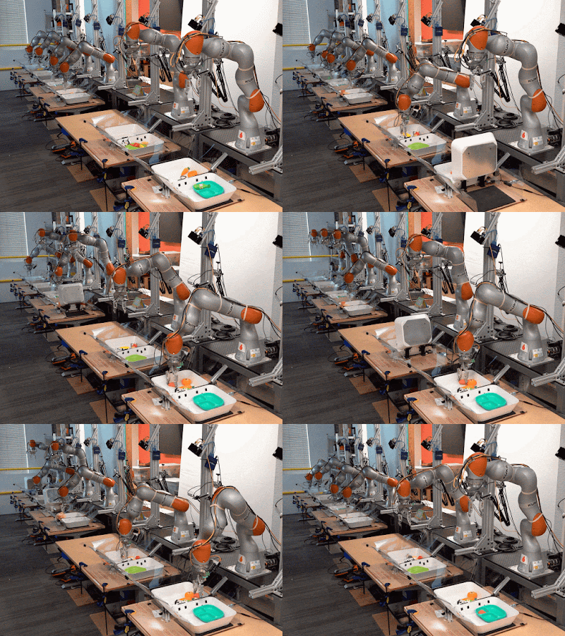
Multi-task data collection across multiple robots where different robots collect data for different tasks.

In other large-scale machine learning domains, such as natural language processing and computer vision, a number of strategies have been applied to amortize the effort of learning over multiple skills. For example, pre-training on large natural language datasets can enable few- or zero-shot learning of multiple tasks, such as question answering and sentiment analysis. However, because robots collect their own data, robotic skill learning presents a unique set of opportunities and challenges. Automating this process is a large engineering endeavour, and effectively reusing past robotic data collected by different robots remains an open problem.

Today we present two new advances for robotic RL at scale, MT-Opt, a new multi-task RL system for automated data collection and multi-task RL training, and Actionable Models, which leverages the acquired data for goal-conditioned RL. MT-Opt introduces a scalable data-collection mechanism that is used to collect over 800,000 episodes of various tasks on real robots and demonstrates a successful application of multi-task RL that yields ~3x average improvement over baseline. Additionally, it enables robots to master new tasks quickly through use of its extensive multi-task dataset (new task fine-tuning in <1 day of data collection). Actionable Models enables learning in the absence of specific tasks and rewards by training an implicit model of the world that is also an actionable robotic policy. This drastically increases the number of tasks the robot can perform (via visual goal specification) and enables more efficient learning of downstream tasks.

Large-Scale Multi-Task Data Collection System
The cornerstone for both MT-Opt and Actionable Models is the volume and quality of training data. To collect diverse, multi-task data at scale, users need a way to specify tasks, decide for which tasks to collect the data, and finally, manage and balance the resulting dataset. To that end, we create a scalable and intuitive multi-task success detector using data from all of the chosen tasks. The multi-task success is trained using supervised learning to detect the outcome of a given task and it allows users to quickly define new tasks and their rewards. When this success detector is being applied to collect data, it is periodically updated to accommodate distribution shifts caused by various real-world factors, such as varying lighting conditions, changing background surroundings, and novel states that the robots discover.

Second, we simultaneously collect data for multiple distinct tasks across multiple robots by using solutions to easier tasks to effectively bootstrap learning of more complex tasks. This allows training of a policy for the harder tasks and improves the data collected for them. As such, the amount of per-task data and the number of successful episodes for each task grows over time. To further improve the performance, we focus data collection on underperforming tasks, rather than collecting data uniformly across tasks.

This system collected 9600 robot hours of data (from 57 continuous data collection days on seven robots). However, while this data collection strategy was effective at collecting data for a large number of tasks, the success rate and data volume was imbalanced between tasks.

Learning with MT-Opt
We address the data collection imbalance by transferring data across tasks and re-balancing the per-task data. The robots generate episodes that are labelled as success or failure for each task and are then copied and shared across other tasks. The balanced batch of episodes is then sent to our multi-task RL training pipeline to train the MT-Opt policy.

Data sharing and task re-balancing strategy used by MT-Opt. The robots generate episodes which then get labelled as success or failure for the current task and are then shared across other tasks.

MT-Opt uses Q-learning, a popular RL method that learns a function that estimates the future sum of rewards, called the Q-function. The learned policy then picks the action that maximizes this learned Q-function. For multi-task policy training, we specify the task as an extra input to a large Q-learning network (inspired by our previous work on large-scale single-task learning with QT-Opt) and then train all of the tasks simultaneously with offline RL using the entire multi-task dataset. In this way, MT-Opt is able to train on a wide variety of skills that include picking specific objects, placing them into various fixtures, aligning items on a rack, rearranging and covering objects with towels, etc.

Compared to single-task baselines, MT-Opt performs similarly on the tasks that have the most data and significantly improves performance on underrepresented tasks. So, for a generic lifting task, which has the most supporting data, MT-Opt achieved an 89% success rate (compared to 88% for QT-Opt) and achieved a 50% average success rate across rare tasks, compared to 1% with a single-task QT-Opt baseline and 18% using a naïve, multi-task QT-Opt baseline. Using MT-Opt not only enables zero-shot generalization to new but similar tasks, but also can quickly (in about 1 day of data collection on seven robots) be fine-tuned to new, previously unseen tasks. For example, when applied to an unseen towel-covering task, the system achieved a zero-shot success rate of 92% for towel-picking and 79% for object-covering, which wasn’t present in the original dataset.

Example tasks that MT-Opt is able to learn, such as instance and indiscriminate grasping, chasing, placing, aligning and rearranging.
Towel-covering task that was not present in the original dataset. We fine-tune MT-Opt on this novel task in 1 day to achieve a high (>90%) success rate.

Learning with Actionable Models
While supplying a rigid definition of tasks facilitates autonomous data collection for MT-Opt, it limits the number of learnable behaviors to a fixed set. To enable learning a wider range of tasks from the same data, we use goal-conditioned learning, i.e., learning to reach given goal configurations of a scene in front of the robot, which we specify with goal images. In contrast to explicit model-based methods that learn predictive models of future world observations, or approaches that employ online data collection, this approach learns goal-conditioned policies via offline model-free RL.

To learn to reach any goal state, we perform hindsight relabeling of all trajectories and sub-sequences in our collected dataset and train a goal-conditioned Q-function in a fully offline manner (in contrast to learning online using a fixed set of success examples as in recursive classification). One challenge in this setting is the distributional shift caused by learning only from “positive” hindsight relabeled examples. This we address by employing a conservative strategy to minimize Q-values of unseen actions using artificial negative actions. Furthermore, to enable reaching temporary-extended goals, we introduce a technique for chaining goals across multiple episodes.

Actionable Models relabel sub-sequences with all intermediate goals and regularize Q-values with artificial negative actions.

Training with Actionable Models allows the system to learn a large repertoire of visually indicated skills, such as object grasping, container placing and object rearrangement. The model is also able to generalize to novel objects and visual objectives not seen in the training data, which demonstrates its ability to learn general functional knowledge about the world. We also show that downstream reinforcement learning tasks can be learned more efficiently by either fine-tuning a pre-trained goal-conditioned model or through a goal-reaching auxiliary objective during training.

Example tasks (specified by goal-images) that our Actionable Model is able to learn.

Conclusion
The results of both MT-Opt and Actionable Models indicate that it is possible to collect and then learn many distinct tasks from large diverse real-robot datasets within a single model, effectively amortizing the cost of learning across many skills. We see this an important step towards general robot learning systems that can be further scaled up to perform many useful services and serve as a starting point for learning downstream tasks.

This post is based on two papers, "MT-Opt: Continuous Multi-Task Robotic Reinforcement Learning at Scale" and "Actionable Models: Unsupervised Offline Reinforcement Learning of Robotic Skills," with additional information and videos on the project websites for MT-Opt and Actionable Models.

Acknowledgements
This research was conducted by Dmitry Kalashnikov, Jake Varley, Yevgen Chebotar, Ben Swanson, Rico Jonschkowski, Chelsea Finn, Sergey Levine, Yao Lu, Alex Irpan, Ben Eysenbach, Ryan Julian and Ted Xiao. We’d like to give special thanks to Josh Weaver, Noah Brown, Khem Holden, Linda Luu and Brandon Kinman for their robot operation support; Anthony Brohan for help with distributed learning and testing infrastructure; Tom Small for help with videos and project media; Julian Ibarz, Kanishka Rao, Vikas Sindhwani and Vincent Vanhoucke for their support; Tuna Toksoz and Garrett Peake for improving the bin reset mechanisms; Satoshi Kataoka, Michael Ahn, and Ken Oslund for help with the underlying control stack, and the rest of the Robotics at Google team for their overall support and encouragement. All the above contributions were incredibly enabling for this research.

Source: Google AI Blog


Recursive Classification: Replacing Rewards with Examples in RL

A general goal of robotics research is to design systems that can assist in a variety of tasks that can potentially improve daily life. Most reinforcement learning algorithms for teaching agents to perform new tasks require a reward function, which provides positive feedback to the agent for taking actions that lead to good outcomes. However, actually specifying these reward functions can be quite tedious and can be very difficult to define for situations without a clear objective, such as whether a room is clean or if a door is sufficiently shut. Even for tasks that are easy to describe, actually measuring whether the task has been solved can be difficult and may require adding many sensors to a robot's environment.

Alternatively, training a model using examples, called example-based control, has the potential to overcome the limitations of approaches that rely on traditional reward functions. This new problem statement is most similar to prior methods based on "success detectors", and efficient algorithms for example-based control could enable non-expert users to teach robots to perform new tasks, without the need for coding expertise, knowledge of reward function design, or the installation of environmental sensors.

In "Replacing Rewards with Examples: Example-Based Policy Search via Recursive Classification," we propose a machine learning algorithm for teaching agents how to solve new tasks by providing examples of success (e.g., if “success” examples show a nail embedded into a wall, the agent will learn to pick up a hammer and knock nails into the wall). This algorithm, recursive classification of examples (RCE), does not rely on hand-crafted reward functions, distance functions, or features, but rather learns to solve tasks directly from data, requiring the agent to learn how to solve the entire task by itself, without requiring examples of any intermediate states. Using a version of temporal difference learning — similar to Q-learning, but replacing the typical reward function term using only examples of success — RCE outperforms prior approaches based on imitation learning on simulated robotics tasks. Coupled with theoretical guarantees similar to those for reward-based learning, the proposed method offers a user-friendly alternative for teaching robots new tasks.

Top: To teach a robot to hammer a nail into a wall, most reinforcement learning algorithms require that the user define a reward function. Bottom: The example-based control method uses examples of what the world looks like when a task is completed to teach the robot to solve the task, e.g., examples where the nail is already hammered into the wall.

Example-Based Control vs Imitation Learning
While the example-based control method is similar to imitation learning, there is an important distinction — it does not require expert demonstrations. In fact, the user can actually be quite bad at performing the task themselves, as long as they can look back and pick out the small fraction of states where they did happen to solve the task.

Additionally, whereas previous research used a stage-wise approach in which the model first uses success examples to learn a reward function and then applies that reward function with an off-the-shelf reinforcement learning algorithm, RCE learns directly from the examples and skips the intermediate step of defining the reward function. Doing so avoids potential bugs and bypasses the process of defining the hyperparameters associated with learning a reward function (such as how often to update the reward function or how to regularize it) and, when debugging, removes the need to examine code related to learning the reward function.

Recursive Classification of Examples
The intuition behind the RCE approach is simple: the model should predict whether the agent will solve the task in the future, given the current state of the world and the action that the agent is taking. If there were data that specified which state-action pairs lead to future success and which state-action pairs lead to future failure, then one could solve this problem using standard supervised learning. However, when the only data available consists of success examples, the system doesn’t know which states and actions led to success, and while the system also has experience interacting with the environment, this experience isn't labeled as leading to success or not.

Left: The key idea is to learn a future success classifier that predicts for every state (circle) in a trajectory whether the task will be solved in the future (thumbs up/down). Right: In the example-based control approach, the model is provided only with unlabeled experience (grey circles) and success examples (green circles), so one cannot apply standard supervised learning. Instead, the model uses the success examples to automatically label the unlabeled experience.

Nonetheless, one can piece together what these data would look like, if it were available. First, by definition, a successful example must be one that solves the given task. Second, even though it is unknown whether an arbitrary state-action pair will lead to success in solving a task, it is possible to estimate how likely it is that the task will be solved if the agent started at the next state. If the next state is likely to lead to future success, it can be assumed that the current state is also likely to lead to future success. In effect, this is recursive classification, where the labels are inferred based on predictions at the next time step.

The underlying algorithmic idea of using a model's predictions at a future time step as a label for the current time step closely resembles existing temporal-difference methods, such as Q-learning and successor features. The key difference is that the approach described here does not require a reward function. Nonetheless, we show that this method inherits many of the same theoretical convergence guarantees as temporal difference methods. In practice, implementing RCE requires changing only a few lines of code in an existing Q-learning implementation.

Evaluation
We evaluated the RCE method on a range of challenging robotic manipulation tasks. For example, in one task we required a robotic hand to pick up a hammer and hit a nail into a board. Previous research into this task [1, 2] have used a complex reward function (with terms corresponding to the distance between the hand and the hammer, the distance between the hammer and the nail, and whether the nail has been knocked into the board). In contrast, the RCE method requires only a few observations of what the world would look like if the nail were hammered into the board.

We compared the performance of RCE to a number of prior methods, including those that learn an explicit reward function and those based on imitation learning , all of which struggle to solve this task. This experiment highlights how example-based control makes it easy for users to specify even complex tasks, and demonstrates that recursive classification can successfully solve these sorts of tasks.

Compared with prior methods, the RCE approach solves the task of hammering a nail into a board more reliably that prior approaches based on imitation learning [SQIL, DAC] and those that learn an explicit reward function [VICE, ORIL, PURL].

Conclusion
We have presented a method to teach autonomous agents to perform tasks by providing them with examples of success, rather than meticulously designing reward functions or collecting first-person demonstrations. An important aspect of example-based control, which we discuss in the paper, is what assumptions the system makes about the capabilities of different users. Designing variants of RCE that are robust to differences in users' capabilities may be important for applications in real-world robotics. The code is available, and the project website contains additional videos of the learned behaviors.

Acknowledgements
We thank our co-authors, Ruslan Salakhutdinov and Sergey Levine. We also thank Surya Bhupatiraju, Kamyar Ghasemipour, Max Igl, and Harini Kannan for feedback on this post, and Tom Small for helping to design figures for this post.

Source: Google AI Blog


Leveraging Machine Learning for Game Development

Over the years, online multiplayer games have exploded in popularity, captivating millions of players across the world. This popularity has also exponentially increased demands on game designers, as players expect games to be well-crafted and balanced — after all, it's no fun to play a game where a single strategy beats all the rest.

In order to create a positive gameplay experience, game designers typically tune the balance of a game iteratively:

  1. Stress-test through thousands of play-testing sessions from test users
  2. Incorporate feedback and re-design the game
  3. Repeat 1 & 2 until both the play-testers and game designers are satisfied

This process is not only time-consuming but also imperfect — the more complex the game, the easier it is for subtle flaws to slip through the cracks. When games often have many different roles that can be played, with dozens of interconnecting skills, it makes it all the more difficult to hit the right balance.

Today, we present an approach that leverages machine learning (ML) to adjust game balance by training models to serve as play-testers, and demonstrate this approach on the digital card game prototype Chimera, which we’ve previously shown as a testbed for ML-generated art. By running millions of simulations using trained agents to collect data, this ML-based game testing approach enables game designers to more efficiently make a game more fun, balanced, and aligned with their original vision.
Chimera
We developed Chimera as a game prototype that would heavily lean on machine learning during its development process. For the game itself, we purposefully designed the rules to expand the possibility space, making it difficult to build a traditional hand-crafted AI to play the game.

The gameplay of Chimera revolves around the titular chimeras, creature mash-ups that players aim to strengthen and evolve. The objective of the game is to defeat the opponent's chimera. These are the key points in the game design:

  • Players may play:
    • creatures, which can attack (through their attack stat) or be attacked (against their health stat), or
    • spells, which produce special effects.
  • Creatures are summoned into limited-capacity biomes, which are placed physically on the board space. Each creature has a preferred biome and will take repeated damage if placed on an incorrect biome or a biome that is over capacity.
  • A player controls a single chimera, which starts off in a basic "egg" state and can be evolved and strengthened by absorbing creatures. To do this, the player must also acquire a certain amount of link energy, which is generated from various gameplay mechanics.
  • The game ends when a player has successfully brought the health of the opponent's chimera to 0.

Learning to Play Chimera
As an imperfect information card game with a large state space, we expected Chimera to be a difficult game for an ML model to learn, especially as we were aiming for a relatively simple model. We used an approach inspired by those used by earlier game-playing agents like AlphaGo, in which a convolutional neural network (CNN) is trained to predict the probability of a win when given an arbitrary game state. After training an initial model on games where random moves were chosen, we set the agent to play against itself, iteratively collecting game data, that was then used to train a new agent. With each iteration, the quality of the training data improved, as did the agent’s ability to play the game.
The ML agent's performance against our best hand-crafted AI as training progressed. The initial ML agent (version 0) picked moves randomly.

For the actual game state representation that the model would receive as input, we found that passing an "image" encoding to the CNN resulted in the best performance, beating all benchmark procedural agents and other types of networks (e.g. fully connected). The chosen model architecture is small enough to run on a CPU in reasonable time, which allowed us to download the model weights and run the agent live in a Chimera game client using Unity Barracuda.

An example game state representation used to train the neural network.
In addition to making decisions for the game AI, we also used the model to display the estimated win probability for a player over the course of the game.

Balancing Chimera
This approach enabled us to simulate millions more games than real players would be capable of playing in the same time span. After collecting data from the games played by the best-performing agents, we analyzed the results to find imbalances between the two of the player decks we had designed.

First, the Evasion Link Gen deck was composed of spells and creatures with abilities that generated extra link energy used to evolve a player’s chimera. It also contained spells that enabled creatures to evade attacks. In contrast, the Damage-Heal deck contained creatures of variable strength with spells that focused on healing and inflicting minor damage. Although we had designed these decks to be of equal strength, the Evasion Link Gen deck was winning 60% of the time when played against the Damage-Heal deck.

When we collected various stats related to biomes, creatures, spells, and chimera evolutions, two things immediately jumped out at us:

  1. There was a clear advantage in evolving a chimera — the agent won a majority of the games where it evolved its chimera more than the opponent did. Yet, the average number of evolves per game did not meet our expectations. To make it more of a core game mechanic, we wanted to increase the overall average number of evolves while keeping its usage strategic.
  2. The T-Rex creature was overpowered. Its appearances correlated strongly with wins, and the model would always play the T-Rex regardless of penalties for summoning into an incorrect or overcrowded biome.

From these insights, we made some adjustments to the game. To emphasize chimera evolution as a core mechanism in the game, we decreased the amount of link energy required to evolve a chimera from 3 to 1. We also added a “cool-off” period to the T-Rex creature, doubling the time it took to recover from any of its actions.

Repeating our ‘self-play’ training procedure with the updated rules, we observed that these changes pushed the game in the desired direction — the average number of evolves per game increased, and the T-Rex's dominance faded.

One example comparison of the T-Rex’s influence before and after balancing. The charts present the number of games won (or lost) when a deck initiates a particular spell interaction (e.g., using the “Dodge” spell to benefit a T-Rex). Left: Before the changes, the T-Rex had a strong influence in every metric examined — highest survival rate, most likely to be summoned ignoring penalties, most absorbed creature during wins. Right: After the changes, the T-Rex was much less overpowered.

By weakening the T-Rex, we successfully reduced the Evasion Link Gen deck's reliance on an overpowered creature. Even so, the win ratio between the decks remained at 60/40 rather than 50/50. A closer look at the individual game logs revealed that the gameplay was often less strategic than we would have liked. Searching through our gathered data again, we found several more areas to introduce changes in.

To start, we increased the starting health of both players as well as the amount of health that healing spells could replenish. This was to encourage longer games that would allow a more diverse set of strategies to flourish. In particular, this enabled the Damage-Heal deck to survive long enough to take advantage of its healing strategy. To encourage proper summoning and strategic biome placement, we increased the existing penalties on playing creatures into incorrect or overcrowded biomes. And finally, we decreased the gap between the strongest and weakest creatures through minor attribute adjustments.

New adjustments in place, we arrived at the final game balance stats for these two decks:

Deck Avg # evolves per game    
(before → after)    
Win % (1M games)
(before → after)
Evasion Link Gen     1.54 → 2.16     59.1% → 49.8%
Damage Heal 0.86 → 1.76     40.9% → 50.2%

Conclusion
Normally, identifying imbalances in a newly prototyped game can take months of playtesting. With this approach, we were able to not only discover potential imbalances but also introduce tweaks to mitigate them in a span of days. We found that a relatively simple neural network was sufficient to reach high level performance against humans and traditional game AI. These agents could be leveraged in further ways, such as for coaching new players or discovering unexpected strategies. We hope this work will inspire more exploration in the possibilities of machine learning for game development.

Acknowledgements
This project was conducted in collaboration with many people. Thanks to Ryan Poplin, Maxwell Hannaman, Taylor Steil, Adam Prins, Michal Todorovic, Xuefan Zhou, Aaron Cammarata, Andeep Toor, Trung Le, Erin Hoffman-John, and Colin Boswell. Thanks to everyone who contributed through playtesting, advising on game design, and giving valuable feedback.

Source: Google AI Blog


PAIRED: A New Multi-agent Approach for Adversarial Environment Generation

The effectiveness of any machine learning method is critically dependent on its training data. In the case of reinforcement learning (RL), one can rely either on limited data collected by an agent interacting with the real world, or a simulated training environment that can be used to collect as much data as needed. This latter method of training in simulation is increasingly popular, but it has a problem — the RL agent can learn what is built into the simulator, but tends to be bad at generalizing to tasks that are even slightly different than the ones simulated. And obviously building a simulator that covers all the complexity of the real-world is extremely challenging.

An approach to address this is to automatically create more diverse training environments by randomizing all the parameters of the simulator, a process called domain randomization (DR). However, DR can fail even in very simple environments. For example, in the animation below, the blue agent is trying to navigate to the green goal. The left panel shows an environment created with DR where the positions of the obstacles and goal have been randomized. Many of these DR environments were used to train the agent, which was then transferred to the simple Four Rooms environment in the middle panel. Notice that the agent can’t find the goal. This is because it has not learned to walk around walls. Even though the wall configuration from the Four Rooms example could have been generated randomly in the DR training phase, it’s unlikely. As a result, the agent has not spent enough time training on walls similar to the Four Rooms structure, and is unable to reach the goal.

Domain randomization (left) does not effectively prepare an agent to transfer to previously unseen environments, such as the Four Rooms scenario (middle). To address this, a minimax adversary is used to construct previously unseen environments (right), but can result in creating situations that are impossible to solve.

Instead of just randomizing the environment parameters, one could train a second RL agent to learn how to set the environment parameters. This minimax adversary can be trained to minimize the performance of the first RL agent by finding and exploiting weaknesses in its policy - e.g. building wall configurations it has not encountered before. But again there is a problem. The right panel shows an environment built by a minimax adversary in which it is actually impossible for the agent to reach the goal. While the minimax adversary has succeeded in its task — it has minimized the performance of the original agent — it provides no opportunity for the agent to learn. Using a purely adversarial objective is not well suited to generating training environments, either.

In collaboration with UC Berkeley, we propose a new multi-agent approach for training the adversary in “Emergent Complexity and Zero-shot Transfer via Unsupervised Environment Design”, a publication recently presented at NeurIPS 2020. In this work we present an algorithm, Protagonist Antagonist Induced Regret Environment Design (PAIRED), that is based on minimax regret and prevents the adversary from creating impossible environments, while still enabling it to correct weaknesses in the agent’s policy. PAIRED incentivizes the adversary to tune the difficulty of the generated environments to be just outside the agent’s current abilities, leading to an automatic curriculum of increasingly challenging training tasks. We show that agents trained with PAIRED learn more complex behavior and generalize better to unknown test tasks. We have released open-source code for PAIRED on our GitHub repo.

PAIRED
To flexibly constrain the adversary, PAIRED introduces a third RL agent, which we call the antagonist agent, because it is allied with the adversarial agent, i.e., the one designing the environment. We rename our initial agent, the one navigating the environment, the protagonist. Once the adversary generates an environment, both the protagonist and antagonist play through that environment.

The adversary’s job is to maximize the antagonist’s reward while minimizing the protagonist's reward. This means it must create environments that are feasible (because the antagonist can solve them and get a high score), but challenging to the protagonist (exploit weaknesses in its current policy). The gap between the two rewards is the regret — the adversary tries to maximize the regret, while the protagonist competes to minimize it.

The methods discussed above (domain randomization, minimax regret and PAIRED) can be analyzed using the same theoretical framework, unsupervised environment design (UED), which we describe in detail in the paper. UED draws a connection between environment design and decision theory, enabling us to show that domain randomization is equivalent to the Principle of Insufficient Reason, the minimax adversary follows the Maximin Principle, and PAIRED is optimizing minimax regret. Below, we show how each of these ideas works for environment design:

Domain randomization (a) generates unstructured environments that aren’t tailored to the agent’s learning progress. The minimax adversary (b) may create impossible environments. PAIRED (c) can generate challenging, structured environments, which are still possible for the agent to complete.

Curriculum Generation
What’s interesting about minimax regret is that it incentivizes the adversary to generate a curriculum of initially easy, then increasingly challenging environments. In most RL environments, the reward function will give a higher score for completing the task more efficiently, or in fewer timesteps. When this is true, we can show that regret incentivizes the adversary to create the easiest possible environment the protagonist can’t solve yet. To see this, let’s assume the antagonist is perfect, and always gets the highest score that it possibly can. Meanwhile, the protagonist is terrible, and gets a score of zero on everything. In that case, the regret just depends on the difficulty of the environment. Since easier environments can be completed in fewer timesteps, they allow the antagonist to get a higher score. Therefore, the regret of failing at an easy environment is greater than the regret of failing on a hard environment:

So, by maximizing regret the adversary is searching for easy environments that the protagonist fails to do. Once the protagonist learns to solve each environment, the adversary must move on to finding a slightly harder environment that the protagonist can’t solve. Thus, the adversary generates a curriculum of increasingly difficult tasks.

Results
We can see the curriculum emerging in the learning curves below, which plot the shortest path length of a maze the agents have successfully solved. Unlike minimax or domain randomization, the PAIRED adversary creates a curriculum of increasingly longer, but possible, mazes, enabling PAIRED agents to learn more complex behavior.

But can these different training schemes help an agent generalize better to unknown test tasks? Below, we see the zero-shot transfer performance of each algorithm on a series of challenging test tasks. As the complexity of the transfer environment increases, the performance gap between PAIRED and the baselines widens. For extremely difficult tasks like Labyrinth and Maze, PAIRED is the only method that can occasionally solve the task. These results provide promising evidence that PAIRED can be used to improve generalization for deep RL.

Admittedly, these simple gridworlds do not reflect the complexities of the real world tasks that many RL methods are attempting to solve. We address this in “Adversarial Environment Generation for Learning to Navigate the Web”, which examines the performance of PAIRED when applied to more complex problems, such as teaching RL agents to navigate web pages. We propose an improved version of PAIRED, and show how it can be used to train an adversary to generate a curriculum of increasingly challenging websites:

Above, you can see websites built by the adversary in the early, middle, and late training stages, which progress from using very few elements per page to many simultaneous elements, making the tasks progressively harder. We test whether agents trained on this curriculum can generalize to standardized web navigation tasks, and achieve a 75% success rate, with a 4x improvement over the strongest curriculum learning baseline:

Conclusions
Deep RL is very good at fitting a simulated training environment, but how can we build simulations that cover the complexity of the real world? One solution is to automate this process. We propose Unsupervised Environment Design (UED) as a framework that describes different methods for automatically creating a distribution of training environments, and show that UED subsumes prior work like domain randomization and minimax adversarial training. We think PAIRED is a good approach for UED, because regret maximization leads to a curriculum of increasingly challenging tasks, and prepares agents to transfer successfully to unknown test tasks.

Acknowledgements
We would like to recognize the co-authors of “Emergent Complexity and Zero-shot Transfer via Unsupervised Environment Design”: Michael Dennis, Natasha Jaques, Eugene Vinitsky, Alexandre Bayen, Stuart Russell, Andrew Critch, and Sergey Levine, as well as the co-authors of Adversarial Environment Generation for Learning to Navigate the Web: Izzeddin Gur, Natasha Jaques, Yingjie Miao, Jongwook Choi, Kevin Malta, Manoj Tiwari, Honglak Lee, Aleksandra Faust. In addition, we thank Michael Chang, Marvin Zhang, Dale Schuurmans, Aleksandra Faust, Chase Kew, Jie Tan, Dennis Lee, Kelvin Xu, Abhishek Gupta, Adam Gleave, Rohin Shah, Daniel Filan, Lawrence Chan, Sam Toyer, Tyler Westenbroek, Igor Mordatch, Shane Gu, DJ Strouse, and Max Kleiman-Weiner for discussions that contributed to this work.

Source: Google AI Blog


Mastering Atari with Discrete World Models

Deep reinforcement learning (RL) enables artificial agents to improve their decisions over time. Traditional model-free approaches learn which of the actions are successful in different situations by interacting with the environment through a large amount of trial and error. In contrast, recent advances in deep RL have enabled model-based approaches to learn accurate world models from image inputs and use them for planning. World models can learn from fewer interactions, facilitate generalization from offline data, enable forward-looking exploration, and allow reusing knowledge across multiple tasks.

Despite their intriguing benefits, existing world models (such as SimPLe) have not been accurate enough to compete with the top model-free approaches on the most competitive reinforcement learning benchmarks — to date, the well-established Atari benchmark requires model-free algorithms, such as DQN, IQN, and Rainbow, to reach human-level performance. As a result, many researchers have focused instead on developing task-specific planning methods, such as VPN and MuZero, which learn by predicting sums of expected task rewards. However, these methods are specific to individual tasks and it is unclear how well they would generalize to new tasks or learn from unsupervised datasets. Similar to the recent breakthrough of unsupervised representation learning in computer vision [1, 2], world models aim to learn patterns in the environment that are more general than any particular task to later solve tasks more efficiently.

Today, in collaboration with DeepMind and the University of Toronto, we introduce DreamerV2, the first RL agent based on a world model to achieve human-level performance on the Atari benchmark. It constitutes the second generation of the Dreamer agent that learns behaviors purely within the latent space of a world model trained from pixels. DreamerV2 relies exclusively on general information from the images and accurately predicts future task rewards even when its representations were not influenced by those rewards. Using a single GPU, DreamerV2 outperforms top model-free algorithms with the same compute and sample budget.

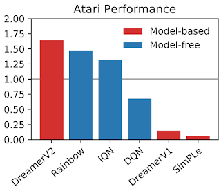
Gamer normalized median score across the 55 Atari games after 200 million steps. DreamerV2 substantially outperforms previous world models. Moreover, it exceeds top model-free agents within the same compute and sample budget.
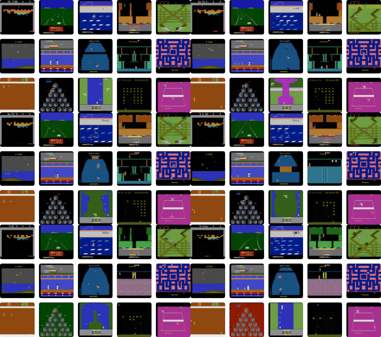
Behaviors learned by DreamerV2 for some of the 55 Atari games. These videos show images from the environment. Video predictions are shown below in the blog post.

An Abstract Model of the World
Just like its predecessor, DreamerV2 learns a world model and uses it to train actor-critic behaviors purely from predicted trajectories. The world model automatically learns to compute compact representations of its images that discover useful concepts, such as object positions, and learns how these concepts change in response to different actions. This lets the agent generate abstractions of its images that ignore irrelevant details and enables massively parallel predictions on a single GPU. During 200 million environment steps, DreamerV2 predicts 468 billion compact states for learning its behavior.

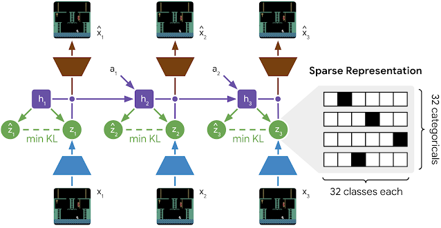
DreamerV2 builds upon the Recurrent State-Space Model (RSSM) that we introduced for PlaNet and was also used for DreamerV1. During training, an encoder turns each image into a stochastic representation that is incorporated into the recurrent state of the world model. Because the representations are stochastic, they do not have access to perfect information about the images and instead extract only what is necessary to make predictions, making the agent robust to unseen images. From each state, a decoder reconstructs the corresponding image to learn general representations. Moreover, a small reward network is trained to rank outcomes during planning. To enable planning without generating images, a predictor learns to guess the stochastic representations without access to the images from which they were computed.

Learning process of the world model used by DreamerV2. The world model maintains recurrent states (h1–h3) that receive actions (a1–a2) and incorporate information about the images (x1–x3) via stochastic representations (z1–z3). A predictor guesses the representations as (ẑ1–ẑ3) without access to the images from which they were generated.

Importantly, DreamerV2 introduces two new techniques to RSSM that lead to a substantially more accurate world model for learning successful policies. The first technique is to represent each image with multiple categorical variables instead of the Gaussian variables used by PlaNet, DreamerV1, and many more world models in the literature [1, 2, 3, 4, 5]. This leads the world model to reason about the world in terms of discrete concepts and enables more accurate predictions of future representations.

The encoder turns each image into 32 distributions over 32 classes each, the meanings of which are determined automatically as the world model learns. The one-hot vectors sampled from these distributions are concatenated to a sparse representation that is passed on to the recurrent state. To backpropagate through the samples, we use straight-through gradients that are easy to implement using automatic differentiation. Representing images with categorical variables allows the predictor to accurately learn the distribution over the one-hot vectors of the possible next images. In contrast, earlier world models that use Gaussian predictors cannot accurately match the distribution over multiple Gaussian representations for the possible next images.

Multiple categoricals that represent possible next images can be accurately predicted by a categorical predictor, whereas a Gaussian predictor is not flexible enough to accurately predict multiple possible Gaussian representations.

The second new technique of DreamerV2 is KL balancing. Many previous world models use the ELBO objective that encourages accurate reconstructions while keeping the stochastic representations (posteriors) close to their predictions (priors) to regularize the amount of information extracted from each image and facilitate generalization. Because the objective is optimized end-to-end, the stochastic representations and their predictions can be made more similar by bringing either of the two towards the other. However, bringing the representations towards their predictions can be problematic when the predictor is not yet accurate. KL balancing lets the predictions move faster toward the representations than vice versa. This results in more accurate predictions, a key to successful planning.

Long-term video predictions of the world model for holdout sequences. Each model receives 5 frames as input (not shown) and then predicts 45 steps forward given only actions. The video predictions are only used to gain insights into the quality of the world model. During planning, only compact representations are predicted, not images.

Measuring Atari Performance
DreamerV2 is the first world model that enables learning successful behaviors with human-level performance on the well-established and competitive Atari benchmark. We select the 55 games that many previous studies have in common and recommend this set of games for future work. Following the standard evaluation protocol, the agents are allowed 200M environment interactions using an action repeat of 4 and sticky actions (25% chance that an action is ignored and the previous action is repeated instead). We compare to the top model-free agents IQN and Rainbow, as well as to the well-known C51 and DQN agents implemented in the Dopamine framework.

Different standards exist for aggregating the scores across the 55 games. Ideally, a new algorithm would perform better under all conditions. For all four aggregation methods, DreamerV2 indeed outperforms all compared model-free algorithms while using the same computational budget.

DreamerV2 outperforms the top model-free agents according to four methods for aggregating scores across the 55 Atari games. We introduce and recommend the Clipped Record Mean (right-most plot) as an informative and robust performance metric.

The first three aggregation methods were previously proposed in the literature. We identify important drawbacks in each and recommend a new aggregation method, the clipped record mean to overcome their drawbacks.

  • Gamer Median. Most commonly, scores for each game are normalized by the performance of a human gamer that was assessed for the DQN paper and the median of the normalized scores of all games is reported. Unfortunately, the median ignores the scores of many simpler and harder games.
  • Gamer Mean. The mean takes the scores for all games into account but is mainly influenced by a small number of games where the human gamer performed poorly. This makes it easy for an algorithm to achieve large normalized scores on some games (e.g., James Bond, Video Pinball) that then dominate the mean.
  • Record Mean. Prior work recommends normalization based on the human world record instead, but such a metric is still overly influenced by a small number of games where it is easy for the artificial agents to outscore the human record.
  • Clipped Record Mean. We introduce a new metric that normalizes scores by the world record and clips them to not exceed the record. This yields an informative and robust metric that takes the performance on all games into account to an approximately equal amount.

While many current algorithms exceed the human gamer baseline, they are still quite far behind the human world record. As shown in the right-most plot above, DreamerV2 leads by achieving 25% of the human record on average across games. Clipping the scores at the record line lets us focus our efforts on developing methods that come closer to the human world record on all of the games rather than exceeding it on just a few games.

What matters and what doesn't
To gain insights into the important components of DreamerV2, we conduct an extensive ablation study. Importantly, we find that categorical representations offer a clear advantage over Gaussian representations despite the fact that Gaussians have been used extensively in prior works. KL balancing provides an even more substantial advantage over the KL regularizer used by most generative models.

By preventing the image reconstruction or reward prediction gradients from shaping the model states, we study their importance for learning successful representations. We find that DreamerV2 relies completely on universal information from the high-dimensional input images and its representations enable accurate reward predictions even when they were not trained using information about the reward. This mirrors the success of unsupervised representation learning in the computer vision community.

Atari performance for various ablations of DreamerV2 (Clipped Record Mean). Categorical representations, KL balancing, and learning about the images are crucial for the success of DreamerV2. Using reward information, that is specific to narrow tasks, offers no additional benefits for learning the world model.

Conclusion
We show how to learn a powerful world model to achieve human-level performance on the competitive Atari benchmark and outperform the top model-free agents. This result demonstrates that world models are a powerful approach for achieving high performance on reinforcement learning problems and are ready to use for practitioners and researchers. We see this as an indication that the success of unsupervised representation learning in computer vision [1, 2] is now starting to be realized in reinforcement learning in the form of world models. An unofficial implementation of DreamerV2 is available on Github and provides a productive starting point for future research projects. We see world models that leverage large offline datasets, long-term memory, hierarchical planning, and directed exploration as exciting avenues for future research.

Acknowledgements
This project is a collaboration with Timothy Lillicrap, Mohammad Norouzi, and Jimmy Ba. We further thank everybody on the Brain Team and beyond who commented on our paper draft and provided feedback at any point throughout the project.

Source: Google AI Blog


Evaluating Design Trade-offs in Visual Model-Based Reinforcement Learning

Model-free reinforcement learning has been successfully demonstrated across a range of domains, including robotics, control, playing games and autonomous vehicles. These systems learn by simple trial and error and thus require a vast number of attempts at a given task before solving it. In contrast, model-based reinforcement learning (MBRL) learns a model of the environment (often referred to as a world model or a dynamics model) that enables the agent to predict the outcomes of potential actions, which reduces the amount of environment interaction needed to solve a task.

In principle, all that is strictly necessary for planning is to predict future rewards, which could then be used to select near-optimal future actions. Nevertheless, many recent methods, such as Dreamer, PlaNet, and SimPLe, additionally leverage the training signal of predicting future images. But is predicting future images actually necessary, or helpful? What benefit do visual MBRL algorithms actually derive from also predicting future images? The computational and representational cost of predicting entire images is considerable, so understanding whether this is actually useful is of profound importance for MBRL research.

In “Models, Pixels, and Rewards: Evaluating Design Trade-offs in Visual Model-Based Reinforcement Learning”, we demonstrate that predicting future images provides a substantial benefit, and is in fact a key ingredient in training successful visual MBRL agents. We developed a new open-source library, called the World Models Library, which enabled us to rigorously evaluate various world model designs to determine the relative impact of image prediction on returned rewards for each.

World Models Library
The World Models Library, designed specifically for visual MBRL training and evaluation, enables the empirical study of the effects of each design decision on the final performance of an agent across multiple tasks on a large scale. The library introduces a platform-agnostic visual MBRL simulation loop and the APIs to seamlessly define new world-models, planners and tasks or to pick and choose from the existing catalog, which includes agents (e.g., PlaNet), video models (e.g., SV2P), and a variety of DeepMind Control tasks and planners, such as CEM and MPPI.

Using the library, developers can study the effect of a varying factor in MBRL, such as the model design or representation space, on the performance of the agent on a suite of tasks. The library supports the training of the agents from scratch, or on a pre-collected set of trajectories, as well as evaluation of a pre-trained agent on a given task. The models, planning algorithms and the tasks can be easily mixed and matched to any desired combination.

To provide the greatest flexibility for users, the library is built using the NumPy interface, which enables different components to be implemented in either TensorFlow, Pytorch or JAX. Please look at this colab for a quick introduction.

Impact of Image Prediction
Using the World Models Library, we trained multiple world models with different levels of image prediction. All of these models use the same input (previously observed images) to predict an image and a reward, but they differ on what percentage of the image they predict. As the number of image pixels predicted by the agent increases, the agent performance as measured by the true reward generally improves.

The input to the model is fixed (previous observed images), but the fraction of the image predicted varies. As can be seen in the graph on the right, increasing the number of predicted pixels significantly improves the performance of the model.

Interestingly, the correlation between reward prediction accuracy and agent performance is not as strong, and in some cases a more accurate reward prediction can even result in lower agent performance. At the same time, there is a strong correlation between image reconstruction error and the performance of the agent.

Correlation between accuracy of image/reward prediction (x-axis) and task performance (y-axis). This graph clearly demonstrates a stronger correlation between image prediction accuracy and task performance.

This phenomenon is directly related to exploration, i.e., when the agent attempts more risky and potentially less rewarding actions in order to collect more information about the unknown options in the environment. This can be shown by testing and comparing models in an offline setup (i.e., learning policies from pre-collected datasets, as opposed to online RL, which learns policies by interacting with an environment). An offline setup ensures that there is no exploration and all of the models are trained on the same data. We observed that models that fit the data better usually perform better in the offline setup, and surprisingly, these may not be the same models that perform the best when learning and exploring from scratch.

Scores achieved by different visual MBRL models across different tasks. The top and bottom half of the graph visualizes the achieved score when trained in the online and offline settings for each task, respectively. Each color is a different model. It is common for a poorly-performing model in the online setting to achieve high scores when trained on pre-collected data (the offline setting) and vice versa.

Conclusion
We have empirically demonstrated that predicting images can substantially improve task performance over models that only predict the expected reward. We have also shown that the accuracy of image prediction strongly correlates with the final task performance of these models. These findings can be used for better model design and can be particularly useful for any future setting where the input space is high-dimensional and collecting data is expensive.

If you'd like to develop your own models and experiments, head to our repository and colab where you'll find instructions on how to reproduce this work and use or extend the World Models Library.

Acknowledgement:
We would like to give special recognition to multiple researchers in the Google Brain team and co-authors of the paper: Mohammad Taghi Saffar, Danijar Hafner, Harini Kannan, Chelsea Finn and Sergey Levine.

Source: Google AI Blog


Estimating the Impact of Training Data with Reinforcement Learning

Recent work suggests that not all data samples are equally useful for training, particularly for deep neural networks (DNNs). Indeed, if a dataset contains low-quality or incorrectly labeled data, one can often improve performance by removing a significant portion of training samples. Moreover, in cases where there is a mismatch between the train and test datasets (e.g., due to difference in train and test location or time), one can also achieve higher performance by carefully restricting samples in the training set to those most relevant for the test scenario. Because of the ubiquity of these scenarios, accurately quantifying the values of training samples has great potential for improving model performance on real-world datasets.


Top: Examples of low-quality samples (noisy/crowd-sourced); Bottom: Examples of a train and test mismatch.

In addition to improving model performance, assigning a quality value to individual data can also enable new use cases. It can be used to suggest better practices for data collection, e.g., what kinds of additional data would benefit the most, and can be used to construct large-scale training datasets more efficiently, e.g., by web searching using the labels as keywords and filtering out less valuable data.

In “Data Valuation Using Deep Reinforcement Learning”, accepted at ICML 2020, we address the challenge of quantifying the value of training data using a novel approach based on meta-learning. Our method integrates data valuation into the training procedure of a predictor model that learns to recognize samples that are more valuable for the given task, improving both predictor and data valuation performance. We have also launched four AI Hub Notebooks that exemplify the use cases of DVRL and are designed to be conveniently adapted to other tasks and datasets, such as domain adaptationcorrupted sample discovery and robust learningtransfer learning on image data and data valuation.

Quantifying the Value of Data
Not all data are equal for a given ML model — some have greater relevance for the task at hand or are more rich in informative content than others. So how does one evaluate the value of a single datum? At the granularity of a full dataset, it is straightforward; one can simply train a model on the entire dataset and use its performance on a test set as its value. However, estimating the value of a single datum is far more difficult, especially for complex models that rely on large-scale datasets, because it is computationally infeasible to re-train and re-evaluate a model on all possible subsets.

To tackle this, researchers have explored permutation-based methods (e.g., influence functions), and game theory-based methods (e.g., data Shapley). However, even the best current methods are far from being computationally feasible for large datasets and complex models, and their data valuation performance is limited. Concurrently, meta learning-based adaptive weight assignment approaches have been developed to estimate the weight values using a meta-objective. But rather than prioritizing learning from high value data samples, their data value mapping is typically based on gradient descent learning or other heuristic approaches that alter the conventional predictor model training dynamics, which can result in performance changes that are unrelated to the value of individual data points.

Data Valuation Using Reinforcement Learning (DVRL)
To infer the data values, we propose a data value estimator (DVE) that estimates data values and selects the most valuable samples to train the predictor model. This selection operation is fundamentally non-differentiable and thus conventional gradient descent-based methods cannot be used. Instead, we propose to use reinforcement learning (RL) such that the supervision of the DVE is based on a reward that quantifies the predictor performance on a small (but clean) validation set. The reward guides the optimization of the policy towards the action of optimal data valuation, given the state and input samples. Here, we treat the predictor model learning and evaluation framework as the environment, a novel application scenario of RL-assisted machine learning.

Training with Data Value Estimation using Reinforcement Learning (DVRL). When training the data value estimator with an accuracy reward, the most valuable samples (denoted with green dots) are used more and more, whereas the least valuable samples (red dots) are used less frequently.

Results
We evaluate the data value estimation quality of DVRL on multiple types of datasets and use cases.

  • Model performance after removing high/low value samples
    Removing low value samples from the training dataset can improve the predictor model performance, especially in the cases where the training dataset contains corrupted samples. On the other hand, removing high value samples, especially if the dataset is small, decreases the performance significantly. Overall, the performance after removing high/low value samples is a strong indicator for the quality of data valuation.
    Accuracy with the removal of most and least valuable samples, where 20% of the labels are noisy by design. By removing such noisy labels as the least valuable samples, a high-quality data valuation method achieves better accuracy. We demonstrate that DVRL outperforms other methods significantly from this perspective.
    DVRL shows the fastest performance degradation after removing the most important samples and the slowest performance degradation after removing the least important samples in most cases, underlining the superiority of DVRL in identifying noisy labels compared to competing methods (Leave-One-Out and Data Shapley).

  • Robust learning with noisy labels
    We consider how reliably DVRL can learn with noisy data in an end-to-end way, without removing the low-value samples. Ideally, noisy samples should get low data values as DVRL converges and a high performance model would be returned.
    Robust learning with noisy labels. Test accuracy for ResNet-32 and WideResNet-28-10 on CIFAR-10 and CIFAR-100 datasets with 40% of uniform random noise on labels. DVRL outperforms other popular methods that are based on meta-learning.
    We show state-of-the-art results with DVRL in minimizing the impact of noisy labels. These also demonstrate that DVRL can scale to complex models and large-scale datasets.

  • Domain adaptation
    We consider the scenario where the training dataset comes from a substantially different distribution from the validation and testing datasets. Data valuation is expected to be beneficial for this task by selecting the samples from the training dataset that best match the distribution of the validation dataset. We focus on the three cases: (1) a training set based on image search results (low-quality web-scraped) applied to the task of predicting skin lesion classification using HAM 10000 data (high-quality medical); (2) an MNIST training set for a digit recognition task on USPS data (different visual domain); (3) e-mail spam data to detect spam applied to an SMS dataset (different task). DVRL yields significant improvements for domain adaptation, by jointly optimizing the data valuator and corresponding predictor model.

Conclusions
We propose a novel meta learning framework for data valuation which determines how likely each training sample will be used in training of the predictor model. Unlike previous works, our method integrates data valuation into the training procedure of the predictor model, allowing the predictor and DVE to improve each other's performance. We model this data value estimation task using a DNN trained through RL with a reward obtained from a small validation set that represents the target task performance. In a computationally-efficient way, DVRL can provide high quality ranking of training data that is useful for domain adaptation, corrupted sample discovery and robust learning. We show that DVRL significantly outperforms alternative methods on diverse types of tasks and datasets.

Acknowledgements
We gratefully acknowledge the contributions of Tomas Pfister.

Source: Google AI Blog