Tag Archives: reinforcement learning

RLDS: An Ecosystem to Generate, Share, and Use Datasets in Reinforcement Learning

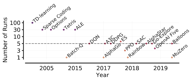
Most reinforcement learning (RL) and sequential decision making algorithms require an agent to generate training data through large amounts of interactions with their environment to achieve optimal performance. This is highly inefficient, especially when generating those interactions is difficult, such as collecting data with a real robot or by interacting with a human expert. This issue can be mitigated by reusing external sources of knowledge, for example, the RL Unplugged Atari dataset, which includes data of a synthetic agent playing Atari games.

However, there are very few of these datasets and a variety of tasks and ways of generating data in sequential decision making (e.g., expert data or noisy demonstrations, human or synthetic interactions, etc.), making it unrealistic and not even desirable for the whole community to work on a small number of representative datasets because these will never be representative enough. Moreover, some of these datasets are released in a form that only works with certain algorithms, which prevents researchers from reusing this data. For example, rather than including the sequence of interactions with the environment, some datasets provide a set of random interactions, making it impossible to reconstruct the temporal relation between them, while others are released in slightly different formats, which can introduce subtle bugs that are very difficult to identify.

In this context, we introduce Reinforcement Learning Datasets (RLDS), and release a suite of tools for recording, replaying, manipulating, annotating and sharing data for sequential decision making, including offline RL, learning from demonstrations, or imitation learning. RLDS makes it easy to share datasets without any loss of information (e.g., keeping the sequence of interactions instead of randomizing them) and to be agnostic to the underlying original format, enabling users to quickly test new algorithms on a wider range of tasks. Additionally, RLDS provides tools for collecting data generated by either synthetic agents (EnvLogger) or humans (RLDS Creator), as well as for inspecting and manipulating the collected data. Ultimately, integration with TensorFlow Datasets (TFDS) facilitates the sharing of RL datasets with the research community.

With RLDS, users can record interactions between an agent and an environment in a lossless and standard format. Then, they can use and transform this data to feed different RL or Sequential Decision Making algorithms, or to perform data analysis.

Dataset Structure
Algorithms in RL, offline RL, or imitation learning may consume data in very different formats, and, if the format of the dataset is unclear, it's easy to introduce bugs caused by misinterpretations of the underlying data. RLDS makes the data format explicit by defining the contents and the meaning of each of the fields of the dataset, and provides tools to re-align and transform this data to fit the format required by any algorithm implementation. In order to define the data format, RLDS takes advantage of the inherently standard structure of RL datasets — i.e., sequences (episodes) of interactions (steps) between agents and environments, where agents can be, for example, rule-based/automation controllers, formal planners, humans, animals, or a combination of these. Each of these steps contains the current observation, the action applied to the current observation, the reward obtained as a result of applying action, and the discount obtained together with reward. Steps also include additional information to indicate whether the step is the first or last of the episode, or if the observation corresponds to a terminal state. Each step and episode may also contain custom metadata that can be used to store environment-related or model-related data.

Producing the Data
Researchers produce datasets by recording the interactions with an environment made by any kind of agent. To maintain its usefulness, raw data is ideally stored in a lossless format by recording all the information that is produced, keeping the temporal relation between the data items (e.g., ordering of steps and episodes), and without making any assumption on how the dataset is going to be used in the future. For this, we release EnvLogger, a software library to log agent-environment interactions in an open format.

EnvLogger is an environment wrapper that records agent–environment interactions and saves them in long-term storage. Although EnvLogger is seamlessly integrated in the RLDS ecosystem, we designed it to be usable as a stand-alone library for greater modularity.

As in most machine learning settings, collecting human data for RL is a time consuming and labor intensive process. The common approach to address this is to use crowd-sourcing, which requires user-friendly access to environments that may be difficult to scale to large numbers of participants. Within the RLDS ecosystem, we release a web-based tool called RLDS Creator, which provides a universal interface to any human-controllable environment through a browser. Users can interact with the environments, e.g., play the Atari games online, and the interactions are recorded and stored such that they can be loaded back later using RLDS for analysis or to train agents.

Sharing the Data
Datasets are often onerous to produce, and sharing with the wider research community not only enables reproducibility of former experiments, but also accelerates research as it makes it easier to run and validate new algorithms on a range of scenarios. For that purpose, RLDS is integrated with TensorFlow Datasets (TFDS), an existing library for sharing datasets within the machine learning community. Once a dataset is part of TFDS, it is indexed in the global TFDS catalog, making it accessible to any researcher by using tfds.load(name_of_dataset), which loads the data either in Tensorflow or in Numpy formats.

TFDS is independent of the underlying format of the original dataset, so any existing dataset with RLDS-compatible format can be used with RLDS, even if it was not originally generated with EnvLogger or RLDS Creator. Also, with TFDS, users keep ownership and full control over their data and all datasets include a citation to credit the dataset authors.

Consuming the Data
Researchers can use the datasets in order to analyze, visualize or train a variety of machine learning algorithms, which, as noted above, may consume data in different formats than how it has been stored. For example, some algorithms, like R2D2 or R2D3, consume full episodes; others, like Behavioral Cloning or ValueDice, consume batches of randomized steps. To enable this, RLDS provides a library of transformations for RL scenarios. These transformations have been optimized, taking into account the nested structure of the RL datasets, and they include auto-batching to accelerate some of these operations. Using those optimized transformations, RLDS users have full flexibility to easily implement some high level functionalities, and the pipelines developed are reusable across RLDS datasets. Example transformations include statistics across the full dataset for selected step fields (or sub-fields) or flexible batching respecting episode boundaries. You can explore the existing transformations in this tutorial and see more complex real examples in this Colab.

Available Datasets
At the moment, the following datasets (compatible with RLDS) are in TFDS:

Our team is committed to quickly expanding this list in the near future and external contributions of new datasets to RLDS and TFDS are welcomed.

Conclusion
The RLDS ecosystem not only improves reproducibility of research in RL and sequential decision making problems, but also enables new research by making it easier to share and reuse data. We hope the capabilities offered by RLDS will initiate a trend of releasing structured RL datasets, holding all the information and covering a wider range of agents and tasks.

Acknowledgements
Besides the authors of this post, this work has been done by Google Research teams in Paris and Zurich in Collaboration with Deepmind. In particular by Sertan Girgin, Damien Vincent, Hanna Yakubovich, Daniel Kenji Toyama, Anita Gergely, Piotr Stanczyk, Raphaël Marinier, Jeremiah Harmsen, Olivier Pietquin and Nikola Momchev. We also want to thank the collaboration of other engineers and researchers who provided feedback and contributed to the project. In particular, George Tucker, Sergio Gomez, Jerry Li, Caglar Gulcehre, Pierre Ruyssen, Etienne Pot, Anton Raichuk, Gabriel Dulac-Arnold, Nino Vieillard, Matthieu Geist, Alexandra Faust, Eugene Brevdo, Tom Granger, Zhitao Gong, Toby Boyd and Tom Small.

Source: Google AI Blog


Decisiveness in Imitation Learning for Robots

Despite considerable progress in robot learning over the past several years, some policies for robotic agents can still struggle to decisively choose actions when trying to imitate precise or complex behaviors. Consider a task in which a robot tries to slide a block across a table to precisely position it into a slot. There are many possible ways to solve this task, each requiring precise movements and corrections. The robot must commit to just one of these options, but must also be capable of changing plans each time the block ends up sliding farther than expected. Although one might expect such a task to be easy, that is often not the case for modern learning-based robots, which often learn behavior that expert observers describe as indecisive or imprecise.

Example of a baseline explicit behavior cloning model struggling on a task where the robot needs to slide a block across a table and then precisely insert it into a fixture.

To encourage robots to be more decisive, researchers often utilize a discretized action space, which forces the robot to choose option A or option B, without oscillating between options. For example, discretization was a key element of our recent Transporter Networks architecture, and is also inherent in many notable achievements by game-playing agents, such as AlphaGo, AlphaStar, and OpenAI’s Dota bot. But discretization brings its own limitations — for robots that operate in the spatially continuous real world, there are at least two downsides to discretization: (i) it limits precision, and (ii) it triggers the curse of dimensionality, since considering discretizations along many different dimensions can dramatically increase memory and compute requirements. Related to this, in 3D computer vision much recent progress has been powered by continuous, rather than discretized, representations.

With the goal of learning decisive policies without the drawbacks of discretization, today we announce our open source implementation of Implicit Behavioral Cloning (Implicit BC), which is a new, simple approach to imitation learning and was presented last week at CoRL 2021. We found that Implicit BC achieves strong results on both simulated benchmark tasks and on real-world robotic tasks that demand precise and decisive behavior. This includes achieving state-of-the-art (SOTA) results on human-expert tasks from our team’s recent benchmark for offline reinforcement learning, D4RL. On six out of seven of these tasks, Implicit BC outperforms the best previous method for offline RL, Conservative Q Learning. Interestingly, Implicit BC achieves these results without requiring any reward information, i.e., it can use relatively simple supervised learning rather than more-complex reinforcement learning.

Implicit Behavioral Cloning
Our approach is a type of behavior cloning, which is arguably the simplest way for robots to learn new skills from demonstrations. In behavior cloning, an agent learns how to mimic an expert’s behavior using standard supervised learning. Traditionally, behavior cloning involves training an explicit neural network (shown below, left), which takes in observations and outputs expert actions.

The key idea behind Implicit BC is to instead train a neural network to take in both observations and actions, and output a single number that is low for expert actions and high for non-expert actions (below, right), turning behavioral cloning into an energy-based modeling problem. After training, the Implicit BC policy generates actions by finding the action input that has the lowest score for a given observation.

Depiction of the difference between explicit (left) and implicit (right) policies. In the implicit policy, the “argmin” means the action that, when paired with a particular observation, minimizes the value of the energy function.

To train Implicit BC models, we use an InfoNCE loss, which trains the network to output low energy for expert actions in the dataset, and high energy for all others (see below). It is interesting to note that this idea of using models that take in both observations and actions is common in reinforcement learning, but not so in supervised policy learning.

Animation of how implicit models can fit discontinuities — in this case, training an implicit model to fit a step (Heaviside) function. Left: 2D plot fitting the black (X) training points — the colors represent the values of the energies (blue is low, brown is high). Middle: 3D plot of the energy model during training. Right: Training loss curve.

Once trained, we find that implicit models are particularly good at precisely modeling discontinuities (above) on which prior explicit models struggle (as in the first figure of this post), resulting in policies that are newly capable of switching decisively between different behaviors.

But why do conventional explicit models struggle? Modern neural networks almost always use continuous activation functions — for example, Tensorflow, Jax, and PyTorch all only ship with continuous activation functions. In attempting to fit discontinuous data, explicit networks built with these activation functions cannot represent discontinuities, so must draw continuous curves between data points. A key aspect of implicit models is that they gain the ability to represent sharp discontinuities, even though the network itself is composed only of continuous layers.

We also establish theoretical foundations for this aspect, specifically a notion of universal approximation. This proves the class of functions that implicit neural networks can represent, which can help justify and guide future research.

Examples of fitting discontinuous functions, for implicit models (top) compared to explicit models (bottom). The red highlighted insets show that implicit models represent discontinuities (a) and (b) while the explicit models must draw continuous lines (c) and (d) in between the discontinuities.

One challenge faced by our initial attempts at this approach was “high action dimensionality”, which means that a robot must decide how to coordinate many motors all at the same time. To scale to high action dimensionality, we use either autoregressive models or Langevin dynamics.

Highlights
In our experiments, we found Implicit BC does particularly well in the real world, including an order of magnitude (10x) better on the 1mm-precision slide-then-insert task compared to a baseline explicit BC model. On this task the implicit model does several consecutive precise adjustments (below) before sliding the block into place. This task demands multiple elements of decisiveness: there are many different possible solutions due to the symmetry of the block and the arbitrary ordering of push maneuvers, and the robot needs to discontinuously decide when the block has been pushed far “enough” before switching to slide it in a different direction. This is in contrast to the indecisiveness that is often associated with continuous-controlled robots.

Example task of sliding a block across a table and precisely inserting it into a slot. These are autonomous behaviors of our Implicit BC policies, using only images (from the shown camera) as input.
A diverse set of different strategies for accomplishing this task. These are autonomous behaviors from our Implicit BC policies, using only images as input.

In another challenging task, the robot needs to sort blocks by color, which presents a large number of possible solutions due to the arbitrary ordering of sorting. On this task the explicit models are customarily indecisive, while implicit models perform considerably better.

Comparison of implicit (left) and explicit (right) BC models on a challenging continuous multi-item sorting task. (4x speed)

In our testing, implicit BC models can also exhibit robust reactive behavior, even when we try to interfere with the robot, despite the model never seeing human hands.

Robust behavior of the implicit BC model despite interfering with the robot.

Overall, we find that Implicit BC policies can achieve strong results compared to state of the art offline reinforcement learning methods across several different task domains. These results include tasks that, challengingly, have either a low number of demonstrations (as few as 19), high observation dimensionality with image-based observations, and/or high action dimensionality up to 30 — which is a large number of actuators to have on a robot.

Policy learning results of Implicit BC compared to baselines across several domains.

Conclusion
Despite its limitations, behavioral cloning with supervised learning remains one of the simplest ways for robots to learn from examples of human behaviors. As we showed here, replacing explicit policies with implicit policies when doing behavioral cloning allows robots to overcome the "struggle of decisiveness", enabling them to imitate much more complex and precise behaviors. While the focus of our results here was on robot learning, the ability of implicit functions to model sharp discontinuities and multimodal labels may have broader interest in other application domains of machine learning as well.

Acknowledgements
Pete and Corey summarized research performed together with other co-authors: Andy Zeng, Oscar Ramirez, Ayzaan Wahid, Laura Downs, Adrian Wong, Johnny Lee, Igor Mordatch, and Jonathan Tompson. The authors would also like to thank Vikas Sindwhani for project direction advice; Steve Xu, Robert Baruch, Arnab Bose for robot software infrastructure; Jake Varley, Alexa Greenberg for ML infrastructure; and Kamyar Ghasemipour, Jon Barron, Eric Jang, Stephen Tu, Sumeet Singh, Jean-Jacques Slotine, Anirudha Majumdar, Vincent Vanhoucke for helpful feedback and discussions.

Source: Google AI Blog


Permutation-Invariant Neural Networks for Reinforcement Learning

“The brain is able to use information coming from the skin as if it were coming from the eyes. We don’t see with the eyes or hear with the ears, these are just the receptors, seeing and hearing in fact goes on in the brain.”
Paul Bach-y-Rita1

People have the amazing ability to use one sensory modality (e.g., touch) to supply environmental information normally gathered by another sense (e.g., vision). This adaptive ability, called sensory substitution, is a phenomenon well-known to neuroscience. While difficult adaptations — such as adjusting to seeing things upside-down, learning to ride a “backwards” bicycle, or learning to “see” by interpreting visual information emitted from a grid of electrodes placed on one’s tongue — require anywhere from weeks, months or even years to attain mastery, people are able to eventually adjust to sensory substitutions.

Examples of Sensory Substitution. Left: Tongue Display Unit (Maris and Bach-y-Rita, 2001; Image: Kaczmarek, 2011). Right: “Upside down goggles” initially conceived by Erismann and Kohler in 1931. (Image Wikipedia).

In contrast, most neural networks are not able to adapt to sensory substitutions at all. For instance, most reinforcement learning (RL) agents require their inputs to be in a pre-specified format, or else they will fail. They expect fixed-size inputs and assume that each element of the input carries a precise meaning, such as the pixel intensity at a specified location, or state information, like position or velocity. In popular RL benchmark tasks (e.g., Ant or Cart-pole), an agent trained using current RL algorithms will fail if its sensory inputs are changed or if the agent is fed additional noisy inputs that are unrelated to the task at hand.

In “The Sensory Neuron as a Transformer: Permutation-Invariant Neural Networks for Reinforcement Learning”, a spotlight paper at NeurIPS 2021, we explore permutation invariant neural network agents, which require each of their sensory neurons (receptors that receive sensory inputs from the environment) to figure out the meaning and context of its input signal, rather than explicitly assuming a fixed meaning. Our experiments show that such agents are robust to observations that contain additional redundant or noisy information, and to observations that are corrupt and incomplete.

Permutation invariant reinforcement learning agents adapting to sensory substitutions. Left: The ordering of the ant’s 28 observations are randomly shuffled every 200 time-steps. Unlike the standard policy, our policy is not affected by the suddenly permuted inputs. Right: Cart-pole agent given many redundant noisy inputs (Interactive web-demo).

In addition to adapting to sensory substitutions in state-observation environments (like the ant and cart-pole examples), we show that these agents can also adapt to sensory substitutions in complex visual-observation environments (such as a CarRacing game that uses only pixel observations) and can perform when the stream of input images is constantly being reshuffled:

We partition the visual input from CarRacing into a 2D grid of small patches, and shuffled their ordering. Without any additional training, our agent still performs even when the original training background (left) is replaced with new images (right).

Method
Our approach takes observations from the environment at each time-step and feeds each element of the observation into distinct, but identical neural networks (called “sensory neurons”), each with no fixed relationship with one another. Each sensory neuron integrates over time information from only their particular sensory input channel. Because each sensory neuron receives only a small part of the full picture, they need to self-organize through communication in order for a global coherent behavior to emerge.

Illustration of observation segmentation.We segment each input into elements, which are then fed to independent sensory neurons. For non-vision tasks where the inputs are usually 1D vectors, each element is a scalar. For vision tasks, we crop each input image into non-overlapping patches.

We encourage neurons to communicate with each other by training them to broadcast messages. While receiving information locally, each individual sensory neuron also continually broadcasts an output message at each time-step. These messages are consolidated and combined into an output vector, called the global latent code, using an attention mechanism similar to that applied in the Transformer architecture. A policy network then uses the global latent code to produce the action that the agent will use to interact with the environment. This action is also fed back into each sensory neuron in the next time-step, closing the communication loop.

Overview of the permutation-invariant RL method. We first feed each individual observation (ot) into a particular sensory neuron (along with the agent’s previous action, at-1). Each neuron then produces and broadcasts a message independently, and an attention mechanism summarizes them into a global latent code (mt) that is given to the agent's downstream policy network (?) to produce the agent’s action at.

Why is this system permutation invariant? Each sensory neuron is an identical neural network that is not confined to only process information from one particular sensory input. In fact, in our setup, the inputs to each sensory neuron are not defined. Instead, each neuron must figure out the meaning of its input signal by paying attention to the inputs received by the other sensory neurons, rather than explicitly assuming a fixed meaning. This encourages the agent to process the entire input as an unordered set, making the system to be permutation invariant to its input. Furthermore, in principle, the agent can use as many sensory neurons as required, thus enabling it to process observations of arbitrary length. Both of these properties will help the agent adapt to sensory substitutions.

Results
We demonstrate the robustness and flexibility of this approach in simpler, state-observation environments, where the observations the agent receives as inputs are low-dimensional vectors holding information about the agent’s states, such as the position or velocity of its components. The agent in the popular Ant locomotion task has a total of 28 inputs with information that includes positions and velocities. We shuffle the order of the input vector several times during a trial and show that the agent is rapidly able to adapt and is still able to walk forward.

In cart-pole, the agent’s goal is to swing up a cart-pole mounted at the center of the cart and balance it upright. Normally the agent sees only five inputs, but we modify the cartpole environment to provide 15 shuffled input signals, 10 of which are pure noise, and the remainder of which are the actual observations from the environment. The agent is still able to perform the task, demonstrating the system’s capacity to work with a large number of inputs and attend only to channels it deems useful. Such flexibility may find useful applications for processing a large unspecified number of signals, most of which are noise, from ill-defined systems.

We also apply this approach to high-dimensional vision-based environments where the observation is a stream of pixel images. Here, we investigate screen-shuffled versions of vision-based RL environments, where each observation frame is divided into a grid of patches, and like a puzzle, the agent must process the patches in a shuffled order to determine a course of action to take. To demonstrate our approach on vision-based tasks, we created a shuffled version of Atari Pong.

Shuffled Pong results. Left: Pong agent trained to play using only 30% of the patches matches performance of Atari opponent. Right: Without extra training, when we give the agent more puzzle pieces, its performance increases.

Here the agent’s input is a variable-length list of patches, so unlike typical RL agents, the agent only gets to “see” a subset of patches from the screen. In the puzzle pong experiment, we pass to the agent a random sample of patches across the screen, which are then fixed through the remainder of the game. We find that we can discard 70% of the patches (at these fixed-random locations) and still train the agent to perform well against the built-in Atari opponent. Interestingly, if we then reveal additional information to the agent (e.g., allowing it access to more image patches), its performance increases, even without additional training. When the agent receives all the patches, in shuffled order, it wins 100% of the time, achieving the same result with agents that are trained while seeing the entire screen.

We find that imposing additional difficulty during training by using unordered observations has additional benefits, such as improving generalization to unseen variations of the task, like when the background of the CarRacing training environment is replaced with a novel image.

Shuffled CarRacing results. The agent has learned to focus its attention (indicated by the highlighted patches) on the road boundaries. Left: Training environment. Right: Test environment with new background.

Conclusion
The permutation invariant neural network agents presented here can handle ill-defined, varying observation spaces. Our agents are robust to observations that contain redundant or noisy information, or observations that are corrupt and incomplete. We believe that permutation invariant systems open up numerous possibilities in reinforcement learning.

If you’re interested to learn more about this work, we invite readers to read our interactive article (pdf version) or watch our video. We also released code to reproduce our experiments.


1Quoted in Livewired, by David Eagleman.  

Source: Google AI Blog


RLiable: Towards Reliable Evaluation & Reporting in Reinforcement Learning

Reinforcement learning (RL) is an area of machine learning that focuses on learning from experiences to solve decision making tasks. While the field of RL has made great progress, resulting in impressive empirical results on complex tasks, such as playing video games, flying stratospheric balloons and designing hardware chips, it is becoming increasingly apparent that the current standards for empirical evaluation might give a false sense of fast scientific progress while slowing it down.

To that end, in “Deep RL at the Edge of the Statistical Precipice”, accepted as an oral presentation at NeurIPS 2021, we discuss how statistical uncertainty of results needs to be considered, especially when using only a few training runs, in order for evaluation in deep RL to be reliable. Specifically, the predominant practice of reporting point estimates ignores this uncertainty and hinders reproducibility of results. Related to this, tables with per-task scores, as are commonly reported, can be overwhelming beyond a few tasks and often omit standard deviations. Furthermore, simple performance metrics like the mean can be dominated by a few outlier tasks, while the median score would remain unaffected even if up to half of the tasks had performance scores of zero. Thus, to increase the field's confidence in reported results with a handful of runs, we propose various statistical tools, including stratified bootstrap confidence intervals, performance profiles, and better metrics, such as interquartile mean and probability of improvement. To help researchers incorporate these tools, we also release an easy-to-use Python library RLiable with a quickstart colab.

Statistical Uncertainty in RL Evaluation
Empirical research in RL relies on evaluating performance on a diverse suite of tasks, such as Atari 2600 video games, to assess progress. Published results on deep RL benchmarks typically compare point estimates of the mean and median scores aggregated across tasks. These scores are typically relative to some defined baseline and optimal performance (e.g., random agent and “average” human performance on Atari games, respectively) so as to make scores comparable across different tasks.

In most RL experiments, there is randomness in the scores obtained from different training runs, so reporting only point estimates does not reveal whether similar results would be obtained with new independent runs. A small number of training runs, coupled with the high variability in performance of deep RL algorithms, often leads to large statistical uncertainty in such point estimates.

The distribution of median human normalized scores on the Atari 100k benchmark, which contains 26 games, for five recently published algorithms, DER, OTR, CURL, two variants of DrQ, and SPR. The reported point estimates of median scores based on a few runs in publications, as shown by dashed lines, do not provide information about the variability in median scores and typically overestimate (e.g., CURL, SPR, DrQ) or underestimate (e.g., DER) the expected median, which can result in erroneous conclusions.

As benchmarks become increasingly more complex, evaluating more than a few runs will be increasingly demanding due to the increased compute and data needed to solve such tasks. For example, five runs on 50 Atari games for 200 million frames takes 1000+ GPU days. Thus, evaluating more runs is not a feasible solution for reducing statistical uncertainty on computationally demanding benchmarks. While prior work has recommended statistical significance tests as a solution, such tests are dichotomous in nature (either “significant” or “not significant”), so they often lack the granularity needed to yield meaningful insights and are widely misinterpreted.

Number of runs in RL papers over the years. Beginning with the Arcade Learning Environment (ALE), the shift toward computationally-demanding benchmarks has led to the practice of evaluating only a handful of runs per task, increasing the statistical uncertainty in point estimates.

Tools for Reliable Evaluation
Any aggregate metric based on a finite number of runs is a random variable, so to take this into account, we advocate for reporting stratified bootstrap confidence intervals (CIs), which predict the likely values of aggregate metrics if the same experiment were repeated with different runs. These CIs allow us to understand the statistical uncertainty and reproducibility of results. Such CIs use the scores on combined runs across tasks. For example, evaluating 3 runs each on Atari 100k, which contains 26 tasks, results in 78 sample scores for uncertainty estimation.

In each task, colored balls denote scores on different runs. To compute statified bootstrap CIs using the percentile method, bootstrap samples are created by randomly sampling scores with replacement proportionately from each task. Then, the distribution of aggregate scores on these samples is the bootstrapping distribution, whose spread around the center gives us the confidence interval.

Most deep RL algorithms often perform better on some tasks and training runs, but aggregate performance metrics can conceal this variability, as shown below.

Data with varied appearance but identical aggregate statistics. Source: Same Stats, Different Graphs.

Instead, we recommend performance profiles, which are typically used for comparing solve times of optimization software. These profiles plot the score distribution across all runs and tasks with uncertainty estimates using stratified bootstrap confidence bands. These plots show the total runs across all tasks that obtain a score above a threshold (?) as a function of the threshold.

Performance profiles correspond to the empirical tail distribution of scores on runs combined across all tasks. Shaded regions show 95% stratified bootstrap confidence bands.

Such profiles allow for qualitative comparisons at a glance. For example, the curve for one algorithm above another means that one algorithm is better than the other. We can also read any score percentile, e.g., the profiles intersect y = 0.5 (dotted line above) at the median score. Furthermore, the area under the profile corresponds to the mean score.

While performance profiles are useful for qualitative comparisons, algorithms rarely outperform other algorithms on all tasks and thus their profiles often intersect, so finer quantitative comparisons require aggregate performance metrics. However, existing metrics have limitations: (1) a single high performing task may dominate the task mean score, while (2) the task median is unaffected by zero scores on nearly half of the tasks and requires a large number of training runs for small statistical uncertainty. To address the above limitations, we recommend two alternatives based on robust statistics: the interquartile mean (IQM) and the optimality gap, both of which can be read as areas under the performance profile, below.

IQM (red) corresponds to the area under the performance profile, shown in blue, between the 25 and 75 percentile scores on the x-axis. Optimality gap (yellow) corresponds to the area between the profile and horizontal line at y = 1 (human performance), for scores less than 1.

As an alternative to median and mean, IQM corresponds to the mean score of the middle 50% of the runs combined across all tasks. It is more robust to outliers than mean, a better indicator of overall performance than median, and results in smaller CIs, and so, requires fewer runs to claim improvements. Another alternative to mean, optimality gap measures how far an algorithm is from optimal performance.

IQM discards the lowest 25% and highest 25% of the combined scores (colored balls) and computes the mean of the remaining 50% scores.

For directly comparing two algorithms, another metric to consider is the average probability of improvement, which describes how likely an improvement over baseline is, regardless of its size. This metric is computed using the Mann-Whitney U-statistic, averaged across tasks.

Re-evaluating Evaluation
Using the above tools for evaluation, we revisit performance evaluations of existing algorithms on widely used RL benchmarks, revealing inconsistencies in prior evaluation. For example, in the Arcade Learning Environment (ALE), a widely recognized RL benchmark, the performance ranking of algorithms changes depending on the choice of aggregate metric. Since performance profiles capture the full picture, they often illustrate why such inconsistencies exist.

Median (left) and IQM (right) human normalized scores on the ALE as a function of the number of environment frames seen during training. IQM results in significantly smaller CIs than median scores.

On DM Control, a popular continuous control benchmark, there are large overlaps in 95% CIs of mean normalized scores for most algorithms.

DM Control Suite results, averaged across six tasks, on the 100k and 500k step benchmark. Since scores are normalized using maximum performance, mean scores correspond to one minus the optimality gap. The ordering of the algorithms is based on their claimed relative performance — all algorithms except Dreamer claimed improvement over at least one algorithm placed below them. Shaded regions show 95% CIs.

Finally, on Procgen, a benchmark for evaluating generalization in RL, the average probability of improvement shows that some claimed improvements are only 50-70% likely, suggesting that some reported improvements could be spurious.

Each row shows the probability that the algorithm X on the left outperforms algorithm Y on the right, given that X was claimed to be better than Y. Shaded region denotes 95% stratified bootstrap CIs.

Conclusion
Our findings on widely-used deep RL benchmarks show that statistical issues can have a large influence on previously reported results. In this work, we take a fresh look at evaluation to improve the interpretation of reported results and standardize experimental reporting. We’d like to emphasize the importance of published papers providing results for all runs to allow for future statistical analyses. To build confidence in your results, please check out our open-source library RLiable and the quickstart colab.

Acknowledgments
This work was done in collaboration with Max Schwarzer, Aaron Courville and Marc G. Bellemare. We’d like to thank Tom Small for an animated figure used in this post. We are also grateful for feedback by several members of the Google Research, Brain Team and DeepMind.

Source: Google AI Blog


Improving Generalization in Reinforcement Learning using Policy Similarity Embeddings

Reinforcement learning (RL) is a sequential decision-making paradigm for training intelligent agents to tackle complex tasks such as robotic locomotion, playing video games, flying stratospheric balloons and designing hardware chips. While RL agents have shown promising results in a variety of activities, it is difficult to transfer the capabilities of these agents to new tasks, even when these tasks are semantically equivalent. For example, consider a jumping task, where an agent, learning from image observations, needs to jump over an obstacle. Deep RL agents trained on a few of these tasks with varying obstacle positions struggle to successfully jump with obstacles at previously unseen locations.

Jumping task: The agent (white block), learning from pixels, needs to jump over an obstacle (gray square). The challenge is to generalize to unseen obstacle positions and floor heights in test tasks using a small number of training tasks. In a given task, the agent needs to time the jump precisely, at a specific distance from the obstacle, otherwise it will eventually hit the obstacle.

In “Contrastive Behavioral Similarity Embeddings for Generalization in Reinforcement Learning”, presented as a spotlight at ICLR 2021, we incorporate the inherent sequential structure in RL into the representation learning process to enhance generalization in unseen tasks. This is orthogonal to the predominant approaches before this work, which were typically adapted from supervised learning, and, as such, largely ignore this sequential aspect. Our approach exploits the fact that an agent, when operating in tasks with similar underlying mechanics, exhibits at least short sequences of behaviors that are similar across these tasks.

Prior work on generalization was typically adapted from supervised learning and revolved around enhancing the learning process. These approaches rarely exploit properties of the sequential aspect such as similarity in actions across temporal observations.

Our approach trains the agent to learn a representation in which states are close when the agent’s optimal behavior in these states and future states are similar. This notion of proximity, which we call behavioral similarity, generalizes to observations across different tasks. To measure behavioral similarity between states across various tasks (e.g., distinct obstacle positions in the jumping task), we introduce the policy similarity metric (PSM), a theoretically motivated state-similarity metric inspired by bisimulation. For example, the image below shows that the agent’s future actions in the two visually different states are the same, making these states similar according to PSM.

Understanding behavioral similarity. The agent (blue icon) needs to obtain the reward while maintaining distance from danger. Even though the initial states are visually different, they are similar in terms of their optimal behavior at current states as well as future states following the current state. Policy similarity metric (PSM) assigns high similarity to such behaviorally similar states and low similarity to dissimilar states.

For enhancing generalization, our approach learns state embeddings, which correspond to neural-network–based representations of task states, that bring together behaviorally similar states (such as in the figure above) while pushing behaviorally dissimilar states apart. To do so, we present contrastive metric embeddings (CMEs) that harness the benefits of contrastive learning for learning representations based on a state-similarity metric. We instantiate contrastive embeddings with the policy similarity metric (PSM) to learn policy similarity embeddings (PSEs). PSEs assign similar representations to states with similar behavior at both those states and future states, such as the two initial states shown in the image above.

As shown in the results below, PSEs considerably enhance generalization on the jumping task from pixels mentioned earlier, outperforming prior methods.

Method Grid Configuration
“Wide” “Narrow” “Random”
Regularization 17.2 (2.2) 10.2 (4.6) 9.3 ( 5.4)
PSEs 33.6 (10.0) 9.3 (5.3) 37.7 (10.4)
Data Augmentation    50.7 (24.2)       33.7 (11.8)       71.3 (15.6)   
Data Aug. + Bisimulation    41.4 (17.6) 17.4 (6.7) 33.4 (15.6)
Data Aug. + PSEs 87.0 (10.1) 52.4 (5.8) 83.4 (10.1)
Jumping Task Results: Percentage (%) of test tasks solved by different methods without and with data augmentation. The “wide”, “narrow”, and “random” grids are configurations shown in the figure below containing 18 training tasks and 268 test tasks. We report average performance across 100 runs with different random initializations, with standard deviation in parentheses.
Jumping Task Grid Configurations: Visualization of average performance of PSEs with data augmentation across different configurations. For each grid configuration, the height varies along the y-axis (11 heights) while the obstacle position varies along the x-axis (26 locations). The red letter T indicates the training tasks. Beige tiles are tasks PSEs solved while black tiles are unsolved tasks, in conjunction with data augmentation.

We also visualize the representations learned by PSEs and baseline methods by projecting them to 2D points with UMAP, a popular visualization technique for high dimensional data. As shown by the visualization, PSEs cluster behaviorally-similar states together and dissimilar states apart, unlike prior methods. Furthermore, PSEs partition the states into two sets: (1) all states before the jump and (2) states where actions do not affect the outcome (states after jump).

Visualizing learned representations. (a) Optimal trajectories on the jumping task (visualized as coloured blocks) with varying obstacle positions. Points with the same number label correspond to the same distance of the agent from the obstacle, the underlying optimal invariant feature across various jumping tasks. (b-d) We visualize the hidden representations using UMAP, where the color of points indicate the tasks of the corresponding observations. (b) PSEs capture the correct invariant feature as can be seen from points with the same number label being clustered together. That is, after the jump action (numbered block 2), all other actions (non-numbered blocks) are similar as shown by the overlapping curve. Contrary to PSEs, baselines including (c) l2-loss embeddings (instead of contrastive loss) and (d) reward-based bisimulation metrics do not put behaviorally similar states with similar number labels together. Poor generalization for (c, d) is likely due to states with the similar optimal behavior ending up with distant embeddings.

Conclusion
Overall, this work shows the benefits of exploiting the inherent structure in RL for learning effective representations. Specifically, this work advances generalization in RL by two contributions: the policy similarity metric and contrastive metric embeddings. PSEs combine these two ideas to enhance generalization. Exciting avenues for future work include finding better ways for defining behavior similarity and leveraging this structure for representation learning.

Acknowledgements
This is a joint work with Pablo Samuel Castro, Marlos C. Machado and Marc G. Bellemare. We would also like to thank David Ha, Ankit Anand, Alex Irpan, Rico Jonschkowski, Richard Song, Ofir Nachum, Dale Schuurmans, Aleksandra Faust and Dibya Ghosh for their insightful comments on this work.

Source: Google AI Blog


Speeding Up Reinforcement Learning with a New Physics Simulation Engine

Reinforcement learning (RL) is a popular method for teaching robots to navigate and manipulate the physical world, which itself can be simplified and expressed as interactions between rigid bodies1 (i.e., solid physical objects that do not deform when a force is applied to them). In order to facilitate the collection of training data in a practical amount of time, RL usually leverages simulation, where approximations of any number of complex objects are composed of many rigid bodies connected by joints and powered by actuators. But this poses a challenge: it frequently takes millions to billions of simulation frames for an RL agent to become proficient at even simple tasks, such as walking, using tools, or assembling toy blocks.

While progress has been made to improve training efficiency by recycling simulation frames, some RL tools instead sidestep this problem by distributing the generation of simulation frames across many simulators. These distributed simulation platforms yield impressive results that train very quickly, but they must run on compute clusters with thousands of CPUs or GPUs which are inaccessible to most researchers.

In “Brax - A Differentiable Physics Engine for Large Scale Rigid Body Simulation”, we present a new physics simulation engine that matches the performance of a large compute cluster with just a single TPU or GPU. The engine is designed to both efficiently run thousands of parallel physics simulations alongside a machine learning (ML) algorithm on a single accelerator and scale millions of simulations seamlessly across pods of interconnected accelerators. We’ve open sourced the engine along with reference RL algorithms and simulation environments that are all accessible via Colab. Using this new platform, we demonstrate 100-1000x faster training compared to a traditional workstation setup.

Three typical RL workflows. The left shows a typical workstation flow: on a single machine, with the environment on CPU, training takes hours or days. The middle shows a typical distributed simulation flow: training takes minutes by farming simulation out to thousands of machines. The right shows the Brax flow: learning and large batch simulation occur side by side on a single CPU/GPU chip.

Physics Simulation Engine Design Opportunities
Rigid body physics are used in video games, robotics, molecular dynamics, biomechanics, graphics and animation, and other domains. In order to accurately model such systems, simulators integrate forces from gravity, motor actuation, joint constraints, object collisions, and others to simulate the motion of a physical system across time.

Simulation of three spherical bodies, a wall, two joints, and one actuator. For each simulation timestep, forces and torques are integrated together to update the positions, rotations, and velocities of each physical body.

Taking a closer look at how most physics simulation engines are designed today, there are a few large opportunities to improve efficiency. As we noted above, a typical robotics learning pipeline places a single learner in a tight feedback with many simulations in parallel, but upon analyzing this architecture, one finds that:

  1. This layout imposes an enormous latency bottleneck. Because the data must travel over the network within a datacenter, the learner must wait for 10,000+ nanoseconds to fetch experience from the simulator. Were this experience instead already on the same device as the learner’s neural network, latency would drop to <1 nanosecond.
  2. The computation necessary for training the agent (one simulation step, followed by one update of the agent’s neural network) is overshadowed by the computation spent packaging the data (i.e., marshalling data within the engine, then into a wire format such as protobuf, then into TCP buffers, and then undoing all these steps on the learner side).
  3. The computations happening within each simulator are remarkably similar, but not exactly the same.

Brax Design
In response to these observations, Brax is designed so that its physics calculations are exactly the same across each of its thousands of parallel environments by ensuring that the simulation is free of branches (i.e., simulation “if” logic that diverges as a result of the environment state). An example of a branch in a physics engine is the application of a contact force between a ball and a wall: different code paths will execute depending on whether the ball is touching the wall. That is, if the ball contacts the wall, separate code for simulating the ball’s bounce off the wall will execute. Brax employs a mix of the following three strategies to avoid branching:

  • Replace the discrete branching logic with a continuous function, such as approximating the ball-wall contact force using a signed distance function. This approach results in the most efficiency gains.
  • Evaluate the branch during JAX’s just-in-time compile. Many branches based on static properties of the environment, such as whether it’s even possible for two objects to collide, may be evaluated prior to simulation time.
  • Run both sides of the branch during simulation but then select only the required results. Because this executes some code that isn’t ultimately used, it wastes operations compared to the above.

Once the calculations are guaranteed to be exactly uniform, the entire training architecture can be reduced in complexity to be executed on a single TPU or GPU. Doing so removes the computational overhead and latency of cross-machine communication. In practice, these changes lower the cost of training by 100x-1000x for comparable workloads.

Brax Environments
Environments are tiny packaged worlds that define a task for an RL agent to learn. Environments contain not only the means to simulate a world, but also functions, such as how to observe the world and the definition of the goal in that world.

A few standard benchmark environments have emerged in recent years for testing new RL algorithms and for evaluating the impact of those algorithms using metrics commonly understood by research scientists. Brax includes four such ready-to-use environments that come from the popular OpenAI gym: Ant, HalfCheetah, Humanoid, and Reacher.


From left to right: Ant, HalfCheetah, Humanoid, and Reacher are popular baseline environments for RL research.

Brax also includes three novel environments: dexterous manipulation of an object (a popular challenge in robotics), generalized locomotion (an agent that goes to a target placed anywhere around it), and a simulation of an industrial robot arm.


Left: Grasp, a claw hand that learns dexterous manipulation. Middle: Fetch, a toy, box-like dog learns a general goal-based locomotion policy. Right: Simulation of UR5e, an industrial robot arm.

Performance Benchmarks
The first step for analyzing Brax’s performance is to measure the speed at which it can simulate large batches of environments, because this is the critical bottleneck to overcome in order for the learner to consume enough experience to learn quickly.

These two graphs below show how many physics steps (updates to the state of the environment) Brax can produce as it is tasked with simulating more and more environments in parallel. The graph on the left shows that Brax scales the number of steps per second linearly with the number of parallel environments, only hitting memory bandwidth bottlenecks at 10,000 environments, which is not only enough for training single agents, but also suitable for training entire populations of agents. The graph on the right shows two things: first, that Brax performs well not only on TPU, but also on high-end GPUs (see the V100 and P100 curves), and second, that by leveraging JAX’s device parallelism primitives, Brax scales seamlessly across multiple devices, reaching hundreds of millions of physics steps per second (see the TPUv3 8x8 curve, which is 64 TPUv3 chips directly connected to each other over a high speed interconnect) .

Left: Scaling of the simulation steps per second for each Brax environment on a 4x2 TPU v3. Right: Scaling of the simulation steps per second for several accelerators on the Ant environment.

Another way to analyze Brax’s performance is to measure its impact on the time it takes to run a reinforcement learning experiment on a single workstation. Here we compare Brax training the popular Ant benchmark environment to its OpenAI counterpart, powered by the MuJoCo physics engine.

In the graph below, the blue line represents a standard workstation setup, where a learner runs on the GPU and the simulator runs on the CPU. We see that the time it takes to train an ant to run with reasonable proficiency (a score of 4000 on the y axis) drops from about 3 hours for the blue line, to about 10 seconds using Brax on accelerator hardware. It’s interesting to note that even on CPU alone (the grey line), Brax performs more than an order of magnitude faster, benefitting from learner and simulator both sitting in the same process.

Brax’s optimized PPO versus a standard GPU-backed PPO learning the MuJoCo-Ant-v2 environment, evaluated for 10 million steps. Note the x-axis is log-wallclock-time in seconds. Shaded region indicates lowest and highest performing seeds over 5 replicas, and solid line indicates mean.

Physics Fidelity
Designing a simulator that matches the behavior of the real world is a known hard problem that this work does not address. Nevertheless, it is useful to compare Brax to a reference simulator to ensure it is producing output that is at least as valid. In this case, we again compare Brax to MuJoCo, which is well-regarded for its simulation quality. We expect to see that, all else being equal, a policy has a similar reward trajectory whether trained in MuJoCo or Brax.

MuJoCo-Ant-v2 vs. Brax Ant, showing the number of environment steps plotted against the average episode score achieved for the environment. Both environments were trained with the same standard implementation of SAC. Shaded region indicates lowest and highest performing seeds over five runs, and solid line indicates the mean.

These curves show that as the reward rises at about the same rate for both simulators, both engines compute physics with a comparable level of complexity or difficulty to solve. And as both curves top out at about the same reward, we have confidence that the same general physical limits apply to agents operating to the best of their ability in either simulation.

We can also measure Brax’s ability to conserve linear momentum, angular momentum, and energy.

Linear momentum (left), angular momentum (middle), and energy (right) non-conservation scaling for Brax as well as several other physics engines. The y-axis indicates drift from the expected calculation (higher is smaller drift, which is better), and the x axis indicates the amount of time being simulated.

This measure of physics simulation quality was first proposed by the authors of MuJoCo as a way to understand how the simulation drifts off course as it is tasked with computing larger and larger time steps. Here, Brax performs similarly as its neighbors.

Conclusion
We invite researchers to perform a more qualitative measure of Brax’s physics fidelity by training their own policies in the Brax Training Colab. The learned trajectories are recognizably similar to those seen in OpenAI Gym.

Our work makes fast, scalable RL and robotics research much more accessible — what was formerly only possible via large compute clusters can now be run on workstations, or for free via hosted Google Colaboratory. Our Github repository includes not only the Brax simulation engine, but also a host of reference RL algorithms for fast training. We can’t wait to see what kind of new research Brax enables.

Acknowledgements
We'd like to thank our paper co-authors: Anton Raichuk, Sertan Girgin, Igor Mordatch, and Olivier Bachem. We also thank Erwin Coumans for advice on building physics engines, Blake Hechtman and James Bradbury for providing optimization help with JAX and XLA, and Luke Metz and Shane Gu for their advice. We’d also like to thank Vijay Sundaram, Wright Bagwell, Matt Leffler, Gavin Dodd, Brad Mckee, and Logan Olson, for helping to incubate this project.


1 Due to the complexity of the real world, there is also ongoing research exploring the physics of deformable bodies

Source: Google AI Blog


Reducing the Computational Cost of Deep Reinforcement Learning Research

It is widely accepted that the enormous growth of deep reinforcement learning research, which combines traditional reinforcement learning with deep neural networks, began with the publication of the seminal DQN algorithm. This paper demonstrated the potential of this combination, showing that it could produce agents that could play a number of Atari 2600 games very effectively. Since then, there have been several approaches that have built on and improved the original DQN. The popular Rainbow algorithm combined a number of these recent advances to achieve state-of-the-art performance on the ALE benchmark. This advance, however, came at a very high computational cost, which has the unfortunate side effect of widening the gap between those with ample access to computational resources and those without.

In “Revisiting Rainbow: Promoting more Insightful and Inclusive Deep Reinforcement Learning Research”, to be presented at ICML 2021, we revisit this algorithm on a set of small- and medium-sized tasks. We first discuss the computational cost associated with the Rainbow algorithm. We explore how the same conclusions regarding the benefits of combining the various algorithmic components can be reached with smaller-scale experiments, and further generalize that idea to how research done on a smaller computational budget can provide valuable scientific insights.

The Cost of Rainbow
A major reason for the computational cost of Rainbow is that the standards in academic publishing often require evaluating new algorithms on large benchmarks like ALE, which consists of 57 Atari 2600 games that reinforcement learning agents may learn to play. For a typical game, it takes roughly five days to train a model using a Tesla P100 GPU. Furthermore, if one wants to establish meaningful confidence bounds, it is common to perform at least five independent runs. Thus, to train Rainbow on the full suite of 57 games required around 34,200 GPU hours (or 1425 days) in order to provide convincing empirical performance statistics. In other words, such experiments are only feasible if one is able to train on multiple GPUs in parallel, which can be prohibitive for smaller research groups.

Revisiting Rainbow
As in the original Rainbow paper, we evaluate the effect of adding the following components to the original DQN algorithm: double Q-learning, prioritized experience replay, dueling networks, multi-step learning, distributional RL, and noisy nets.

We evaluate on a set of four classic control environments, which can be fully trained in 10-20 minutes (compared to five days for ALE games):

Upper left: In CartPole, the task is to balance a pole on a cart that the agent can move left and right. Upper right: In Acrobot, there are two arms and two joints, where the agent applies force to the joint between the two arms in order to raise the lower arm above a threshold. Lower left: In LunarLander, the agent is meant to land the spaceship between the two flags. Lower right: In MountainCar, the agent must build up momentum between two hills to drive to the top of the rightmost hill.

We investigated the effect of both independently adding each of the components to DQN, as well as removing each from the full Rainbow algorithm. As in the original Rainbow paper, we find that, in aggregate, the addition of each of these algorithms does improve learning over the base DQN. However, we also found some important differences, such as the fact that distributional RL — commonly thought to be a positive addition on its own — does not always yield improvements on its own. Indeed, in contrast to the ALE results in the Rainbow paper, in the classic control environments, distributional RL only yields an improvement when combined with another component.

Each plot shows the training progress when adding the various components to DQN. The x-axis is training steps,the y-axis is performance (higher is better).
Each plot shows the training progress when removing the various components from Rainbow. The x-axis is training steps,the y-axis is performance (higher is better).

We also re-ran the Rainbow experiments on the MinAtar environment, which consists of a set of five miniaturized Atari games, and found qualitatively similar results. The MinAtar games are roughly 10 times faster to train than the regular Atari 2600 games on which the original Rainbow algorithm was evaluated, but still share some interesting aspects, such as game dynamics and having pixel-based inputs to the agent. As such, they provide a challenging mid-level environment, in between the classic control and the full Atari 2600 games.

When viewed in aggregate, we find our results to be consistent with those of the original Rainbow paper — the impact resulting from each algorithmic component can vary from environment to environment. If we were to suggest a single agent that balances the tradeoffs of the different algorithmic components, our version of Rainbow would likely be consistent with the original, in that combining all components produces a better overall agent. However, there are important details in the variations of the different algorithmic components that merit a more thorough investigation.

Beyond the Rainbow
When DQN was introduced, it made use of the Huber loss and the RMSProp Optimizer. It has been common practice for researchers to use these same choices when building on DQN, as most of their effort is spent on other algorithmic design decisions. In the spirit of reassessing these assumptions, we revisited the loss function and optimizer used by DQN on a lower-cost, small-scale classic control and MinAtar environments. We ran some initial experiments using the Adam optimizer, which has lately been the most popular optimizer choice, combined with a simpler loss function, the mean-squared error loss (MSE). Since the selection of optimizer and loss function is often overlooked when developing a new algorithm, we were surprised to see that we observed a dramatic improvement on all the classic control and MinAtar environments.

We thus decided to evaluate the different ways of combining the two optimizers (RMSProp and Adam) with the two losses (Huber and MSE) on the full ALE suite (60 Atari 2600 games). We found that Adam+MSE is a superior combination than RMSProp+Huber.

Measuring the improvement Adam+MSE gives over the default DQN settings (RMSProp + Huber); higher is better.

Additionally, when comparing the various optimizer-loss combinations, we find that when using RMSProp, the Huber loss tends to perform better than MSE (illustrated by the gap between the solid and dotted orange lines).

Normalized scores aggregated over all 60 Atari 2600 games, comparing the different optimizer-loss combinations.

Conclusion
On a limited computational budget we were able to reproduce, at a high-level, the findings of the Rainbow paper and uncover new and interesting phenomena. Evidently it is much easier to revisit something than to discover it in the first place. Our intent with this work, however, was to argue for the relevance and significance of empirical research on small- and medium-scale environments. We believe that these less computationally intensive environments lend themselves well to a more critical and thorough analysis of the performance, behaviors, and intricacies of new algorithms.

We are by no means calling for less emphasis to be placed on large-scale benchmarks. We are simply urging researchers to consider smaller-scale environments as a valuable tool in their investigations, and reviewers to avoid dismissing empirical work that focuses on smaller-scale environments. By doing so, in addition to reducing the environmental impact of our experiments, we will get both a clearer picture of the research landscape and reduce the barriers for researchers from diverse and often underresourced communities, which can only help make our community and scientific advances stronger.

Acknowledgments
Thank you to Johan, the first author of this paper, for his hard work and persistence in seeing this through! We would also like to thank Marlos C. Machado, Sara Hooker, Matthieu Geist, Nino Vieillard, Hado van Hasselt, Eleni Triantafillou, and Brian Tanner for their insightful comments on this work.

Source: Google AI Blog