Tag Archives: optimization

Measuring the Limits of Data Parallel Training for Neural Networks


Over the past decade, neural networks have achieved state-of-the-art results in a wide variety of prediction tasks, including image classification, machine translation, and speech recognition. These successes have been driven, at least in part, by hardware and software improvements that have significantly accelerated neural network training. Faster training has directly resulted in dramatic improvements to model quality, both by allowing more training data to be processed and by allowing researchers to try new ideas and configurations more rapidly. Today, hardware developments like Cloud TPU Pods are rapidly increasing the amount of computation available for neural network training, which raises the possibility of harnessing additional computation to make neural networks train even faster and facilitate even greater improvements to model quality. But how exactly should we harness this unprecedented amount of computation, and should we always expect more computation to facilitate faster training?

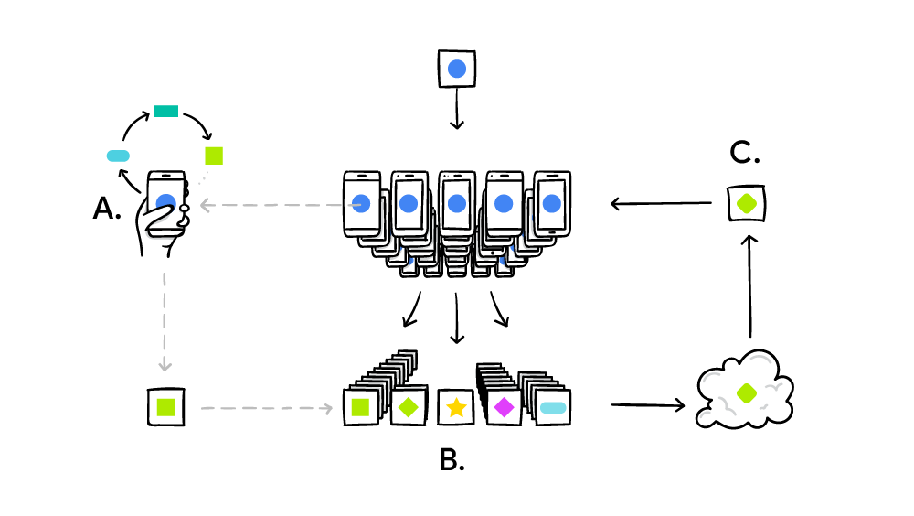
The most common way to utilize massive compute power is to distribute computations between different processors and perform those computations simultaneously. When training neural networks, the primary ways to achieve this are model parallelism, which involves distributing the neural network across different processors, and data parallelism, which involves distributing training examples across different processors and computing updates to the neural network in parallel. While model parallelism makes it possible to train neural networks that are larger than a single processor can support, it usually requires tailoring the model architecture to the available hardware. In contrast, data parallelism is model agnostic and applicable to any neural network architecture – it is the simplest and most widely used technique for parallelizing neural network training. For the most common neural network training algorithms (synchronous stochastic gradient descent and its variants), the scale of data parallelism corresponds to the batch size, the number of training examples used to compute each update to the neural network. But what are the limits of this type of parallelization, and when should we expect to see large speedups?

In "Measuring the Effects of Data Parallelism in Neural Network Training", we investigate the relationship between batch size and training time by running experiments on six different types of neural networks across seven different datasets using three different optimization algorithms ("optimizers"). In total, we trained over 100K individual models across ~450 workloads, and observed a seemingly universal relationship between batch size and training time across all workloads we tested. We also study how this relationship varies with the dataset, neural network architecture, and optimizer, and found extremely large variation between workloads. Additionally, we are excited to share our raw data for further analysis by the research community. The data includes over 71M model evaluations to make up the training curves of all 100K+ individual models we trained, and can be used to reproduce all 24 plots in our paper.

Universal Relationship Between Batch Size and Training Time
In an idealized data parallel system that spends negligible time synchronizing between processors, training time can be measured in the number of training steps (updates to the neural network's parameters). Under this assumption, we observed three distinct scaling regimes in the relationship between batch size and training time: a "perfect scaling" regime where doubling the batch size halves the number of training steps required to reach a target out-of-sample error, followed by a regime of "diminishing returns", and finally a "maximal data parallelism" regime where further increasing the batch size does not reduce training time, even assuming idealized hardware.

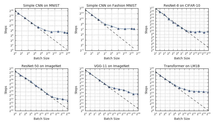
For all workloads we tested, we observed a universal relationship between batch size and training speed with three distinct regimes: perfect scaling (following the dashed line), diminishing returns (diverging from the dashed line), and maximal data parallelism (where the trend plateaus). The transition points between the regimes vary dramatically between different workloads.
Although the basic relationship between batch size and training time appears to be universal, we found that the transition points between the different scaling regimes vary dramatically across neural network architectures and datasets. This means that while simple data parallelism can provide large speedups for some workloads at the limits of today's hardware (e.g. Cloud TPU Pods), and perhaps beyond, some workloads require moving beyond simple data parallelism in order to benefit from the largest scale hardware that exists today, let alone hardware that has yet to be built. For example, in the plot above, ResNet-8 on CIFAR-10 cannot benefit from batch sizes larger than 1,024, whereas ResNet-50 on ImageNet continues to benefit from increasing the batch size up to at least 65,536.

Optimizing Workloads
If one could predict which workloads benefit most from data parallel training, then one could tailor their workloads to make maximal use of the available hardware. However, our results suggest that this will often not be straightforward, because the maximum useful batch size depends, at least somewhat, on every aspect of the workload: the neural network architecture, the dataset, and the optimizer. For example, some neural network architectures can benefit from much larger batch sizes than others, even when trained on the same dataset with the same optimizer. Although this effect sometimes depends on the width and depth of the network, it is inconsistent between different types of network and some networks do not even have obvious notions of "width" and "depth". And while we found that some datasets can benefit from much larger batch sizes than others, these differences are not always explained by the size of the dataset—sometimes smaller datasets benefit more from larger batch sizes than larger datasets.

Left: A transformer neural network scales to much larger batch sizes than an LSTM neural network on the LM1B dataset. Right: The Common Crawl dataset does not benefit from larger batch sizes than the LM1B dataset, even though it is 1,000 times the size.
Perhaps our most promising finding is that even small changes to the optimization algorithm, such as allowing momentum in stochastic gradient descent, can dramatically improve how well training scales with increasing batch size. This raises the possibility of designing new optimizers, or testing the scaling properties of optimizers that we did not consider, to find optimizers that can make maximal use of increased data parallelism.

Future Work
Utilizing additional data parallelism by increasing the batch size is a simple way to produce valuable speedups across a range of workloads, but, for all the workloads we tried, the benefits diminished within the limits of state-of-the-art hardware. However, our results suggest that some optimization algorithms may be able to consistently extend the perfect scaling regime across many models and data sets. Future work could perform the same measurements with other optimizers, beyond the few closely-related ones we tried, to see if any existing optimizer extends perfect scaling across many problems.

Acknowledgements
The authors of this study were Chris Shallue, Jaehoon Lee, Joe Antognini, Jascha Sohl-Dickstein, Roy Frostig and George Dahl (Chris and Jaehoon contributed equally). Many researchers have done work in this area that we have built on, so please see our paper for a full discussion of related work.

Source: Google AI Blog


Google AI Princeton: Current and Future Research


Google has long partnered with academia to advance research, collaborating with universities all over the world on joint research projects which result in novel developments in Computer Science, Engineering, and related fields. Today we announce the latest of these academic partnerships in the form of a new lab, across the street from Princeton University’s historic Nassau Hall, opening early next year. By fostering closer collaborations with faculty and students at Princeton, the lab aims to broaden research in multiple facets of machine learning, focusing its initial research efforts on optimization methods for large-scale machine learning, control theory and reinforcement learning. Below we give a brief overview of the research progress thus far.

Large-Scale Optimization
Imagine you have gone for a mountain hike and have run out of water. You need to get to a lake. How can you do so most efficiently? This is a matter of optimizing your route, and the mathematical analogue of this is the gradient descent method. You therefore move in the direction of steepest descent until you find the nearest lake at the bottom of your path. In the language of optimization, the location of the lake is referred to as a (local) minimum. The trajectory of gradient descent resembles the path, shown below, a thirsty yet avid hiker would take in order to get down to a lake as fast as she can.
Gradient descent (GD), and its randomized version, stochastic gradient descent (SGD), are the methods of choice for optimizing the weights of neural networks. Stacking all of the parameters together, we form a set of cells organized into vectors Let us take a simplistic view and assume that our neural net merely has 5 different parameters. Taking a gradient descent step amounts to subtracting the gradient vector (red) from the current set of parameters (blue) and putting the result back into the parameter vector.
Going back to our avid hiker, suppose she finds an unmarked path that is long and narrow, with limited visibility as she gazes down. If she follows the descent method her path would zig-zag down the hill, as shown in the illustration below on the left. However, she can now make faster progress by exploiting the skewed geometry of the terrain. That is, she can make a bigger leap forward than to the sides. In the context of gradient descent, pacing up is called acceleration. A popular class of acceleration methods is named adaptive regularization, or adaptive preconditioning, first introduced by the AdaGrad algorithm devised in collaboration with Prof. John Duchi from Stanford while he was at Google.
The idea is to change the geometry of the landscape of the optimization objective to make it easier for gradient descent to work. In order to do so, preconditioning methods stretch and rotate the space. The terrain after preconditioning looks like the serene, perfectly spherical lake above on the right, and the descent trajectory is a straight line! Procedurally, instead of subtracting the gradient vectors from the parameters vector per-se, adaptive preconditioning first multiplies the gradient by a 5×5 multicell structure, called a matrix preconditioner, as shown below.
This preconditioning operation yields a stretched and rotated gradient which is then subtracted as before, allowing much faster progress toward a basin. However, there is a downside to preconditioning, namely, its computational cost. Instead of subtracting a 5-dimensional gradient vector from a 5-dimensional parameter vector, the preconditioning transformation itself requires 5×5=25 operations. Suppose we would like to precondition gradients in order to learn a deep network with 10 million parameters. A single preconditioning step would require 100 trillion operations. In order to save computation, a diagonal version in which preconditioning amounts to stretching sans rotation was also introduced in the original AdaGrad paper. The diagonal version was later adopted and modified, yielding another very successful algorithm called Adam.

This simplified diagonal preconditioning imposes only a marginal additional cost to gradient descent. However, oversimplification has its own downside: we are no longer able to rotate our space. Going back to our hiker, if the deep-and-narrow canyon runs from southeast to northwest, she can no longer take large westward leaps. Had we provided her with a “rigged” compass in which the north pole is in the northwest, she could have followed her descent procedure as before. In high dimensions, the analog of compass rigging is full-matrix preconditioning. We thus asked ourselves whether we could devise a preconditioning method that is computationally efficient while allowing for the equivalent of coordinate rotations.

At Google AI Princeton, we developed a new method for full-matrix adaptive preconditioning at roughly the same computational cost as the commonly-used diagonal restriction. Details can be found in the paper, but the key idea behind the method is depicted below. Instead of using a full matrix, we replace the preconditioning matrix by a product of three matrices: a tall & thin matrix, a (small) square matrix, and a short & fat matrix. The vast amount of computation is performed using the smaller matrix. If we have d parameters, instead of a single large d × d matrix, the matrices maintained by GGT (shorthand for the operation Gradient GradientT), the proposed method, are of sizes d × k, k × k, k × d respectively.

For reasonable choices of k, which can be thought of as the “window size” of the algorithm, the computational bottleneck has been mitigated from a single large matrix, to that of a much smaller kkmatrix. In our implementation we typically choose k to be, say, 50, and maintaining the smaller square matrix is significantly less expensive while yielding good empirical performance. When compared to other adaptive methods on standard deep learning tasks, GGT is competitive with AdaGrad and Adam.

Spectral Filtering for Control and Reinforcement Learning
Another broad mission of Google’s research group in Princeton is to develop principled building blocks for decision-making systems. In particular, the group strives to leverage provable guarantees from the field of online learning, which studies the robust (worst-case) guarantees of decision-making algorithms under uncertainty. An online algorithm is said to attain a no-regret guarantee if it learns to make decisions as well as the best "offline" decision in hindsight. Ideas from this field have already enabled many innovations within theoretical computer science, and provide a mathematically elegant framework to study a widely-used technique called boosting. We envision using ideas from online learning to broaden the toolkit of modern reinforcement learning.

With that goal in mind, and in collaboration with researchers and students at Princeton, we developed the algorithmic technique of spectral filtering for estimation and control of linear dynamical systems (see several recent publications). In this setting, noisy observations (e.g., location sensor measurements) are being streamed from an unknown source. The source of the signal is a system whose state evolves over time following a set of linear equations (e.g. Newton's laws). To forecast future signals (prediction), or to perform actions which bring the system to a desired state (control), the usual approach starts with learning the model explicitly (a task termed system identification), which is often slow and inaccurate.

Spectral filtering circumvents the need to model the dynamics explicitly, by reformulating prediction and control as convex programs, enabling provable no-regret guarantees. A major component of the technique is that of a new signal processing transformation. The idea is to summarize the long history of past input signals through convolution with a tailored bank of filters, and then use this representation to predict the dynamical system’s future outputs. Each filter compresses the input signal into a single real number, by taking a weighted combination of the previous inputs.
A set of filters depicted in a plot of filter amplitude versus time. With our technique of spectral filtering, multiple filters are used to predict the state of a linear dynamical system at any given time. Each filter is a set of weights used to summarize past observations, such that combining them in a weighted fashion, over time allows us to accurately predict the system.
The mathematical derivation of these weights (filters) has an interesting connection to the spectral theory of Hankel matrices.

Looking Forward
We are excited about the progress we have made thus far in partnership with Princeton’s faculty and students, and we look forward to the official opening of the lab in the coming weeks. It has long been Google’s view that both industry and academia benefit significantly from an open research culture, and we look forward to our continued close collaboration.

Acknowledgments
The research and results discussed in this post would not have been possible without contributions from the following researchers: Naman Agarwal, Brian Bullins, Xinyi Chen, Udaya Ghai, Tomer Koren, Karan Singh, Cyril Zhang, Yi Zhang, and visiting professor Sham Kakade. Since joining Google earlier this year, the research team has been working remotely from both the Google NYC office as well as the Princeton University campus, and they look forward to moving into the new Google space across from the Princeton campus in the weeks to come.

Source: Google AI Blog


Machine Learning in Google BigQuery


Google BiqQuery allows interactive analysis of large datasets, making it easy for businesses to share meaningful insights and develop solutions based on customer analytics. However, many of the businesses that are using BigQuery aren’t using machine learning to help better understand the data they are generating. This is because data analysts, proficient in SQL, may not have the traditional data science background needed to apply machine learning techniques.

Today we’re announcing BigQuery ML, a capability inside BigQuery that allows data scientists and analysts to build and deploy machine learning models on massive structured or semi-structured datasets. BigQuery ML is a set of simple SQL language extensions which enables users to utilize popular ML capabilities, performing predictive analytics like forecasting sales and creating customer segmentations right at the source, where they already store their data. BigQuery ML additionally sets smart defaults automatically and takes care of data transformation, leading to a seamless and easy to use experience with great results.
When designing the BigQuery ML backend, the team was faced with a dilemma. Transferring large amounts of data from BigQuery servers to special-purpose servers running machine learning algorithms would be time-consuming and would incur an overhead in terms of security and privacy considerations. However, because the core components of gradient descent — an optimization method that is the workhorse of machine learning algorithms — can be implemented using common SQL operations*, we were able to repurpose the existing BigQuery SQL processing engine for BigQuery ML.

Since the BigQuery engine is designed to efficiently scan large datasets rather than randomly draw small samples from them, BigQuery ML is based on the standard (batch) variant of gradient descent rather than the stochastic version. And while stochastic gradient descent is far more common in today’s large-scale machine learning systems, the batch variant has numerous practical advantages.

For example, in-database machine learning systems based on stochastic gradient descent process examples one by one, and can perform poorly when the data is suboptimally ordered. But BigQuery data is often distributed on disk so as to optimize the performance of regular SQL queries, and continually redistributing the data to support stochastic machine learning algorithms would be computationally expensive. In contrast, batch gradient descent is insensitive to the ordering and partitioning of data on disk, thereby completely circumventing this problem. Also, batch methods can be combined with line search techniques from the classical optimization literature, leading to a learning algorithm that is more stable and requires less fine tuning. Using line search with stochastic methods is far trickier. Our implementation also includes support for regularization and preconditioning. For more details, please see our paper.

We hope that you’ll find BigQuery ML useful for many predictive analytics tasks. To try it, visit the BigQuery console and follow the user guide. Creating a model is as simple as:
CREATE MODEL dataset.model_name
OPTIONS(model_type=’linear_reg’, input_label_cols=[‘input_label’])
AS SELECT * FROM input_table;
In the future, we plan to further integrate our gradient descent implementation with BigQuery infrastructure to realize more performance gains. We’re also going to explore other machine learning algorithms that can be easily and efficiently implemented for large-scale problems by leveraging the power of BigQuery.

Acknowledgements
BigQuery ML is the result of a large collaboration across many teams at Google. Key contributors and sponsors include Hossein Ahmadi, Corinna Cortes, Grzegorz Czajkowski, Mingge Deng, Amir Hormati, Abhishek Kashyap, Jing Jing Long, Dan McClary, Chris Meyers, Girishkumar Sabhnani, Vivek Sharma, Jordan Tigani, Chad Verbowski, Jiaxun Wu and Lisa Yin.


* For example, a gradient vector can be computed using the SUM and GROUP BY operators, and the weights of a model can be updated using an INNER JOIN.

Source: Google AI Blog


Realtime tSNE Visualizations with TensorFlow.js


In recent years, the t-distributed Stochastic Neighbor Embedding (tSNE) algorithm has become one of the most used and insightful techniques for exploratory data analysis of high-dimensional data. Used to interpret deep neural network outputs in tools such as the TensorFlow Embedding Projector and TensorBoard, a powerful feature of tSNE is that it reveals clusters of high-dimensional data points at different scales while requiring only minimal tuning of its parameters. Despite these advantages, the computational complexity of the tSNE algorithm limits its application to relatively small datasets. While several evolutions of tSNE have been developed to address this issue (mainly focusing on the scalability of the similarity computations between data points), they have so far not been enough to provide a truly interactive experience when visualizing the evolution of the tSNE embedding for large datasets.

In “Linear tSNE Optimization for the Web”, we present a novel approach to tSNE that heavily relies on modern graphics hardware. Given the linear complexity of the new approach, our method generates embeddings faster than comparable techniques and can even be executed on the client side in a web browser by leveraging GPU capabilities through WebGL. The combination of these two factors allows for real-time interactive visualization of large, high-dimensional datasets. Furthermore, we are releasing this work as an open source library in the TensorFlow.js family in the hopes that the broader research community finds it useful.
Real-time evolution of the tSNE embedding for the complete MNIST dataset with our technique. The dataset contains images of 60,000 handwritten digits. You can find a live demo here.
The aim of tSNE is to cluster small “neighborhoods” of similar data points while also reducing the overall dimensionality of the data so it is more easily visualized. In other words, the tSNE objective function measures how well these neighborhoods of similar data are preserved in the 2 or 3-dimensional space, and arranges them into clusters accordingly.

In previous work, the minimization of the tSNE objective was performed as a N-body simulation problem, in which points are randomly placed in the embedding space and two different types of forces are applied on each point. Attractive forces bring the points closer to the points that are most similar in the high-dimensional space, while repulsive forces push them away from all the neighbors in the embedding.

While the attractive forces are acting on a small subset of points (i.e., similar neighbors), repulsive forces are in effect from all pairs of points. Due to this, tSNE requires significant computation and many iterations of the objective function, which limits the possible dataset size to just a few hundred data points. To improve over a brute force solution, the Barnes-Hut algorithm was used to approximate the repulsive forces and the gradient of the objective function. This allows scaling of the computation to tens of thousand data points, but it requires more than 15 minutes to compute the MNIST embedding in a C++ implementation.

In our paper, we propose a solution to this scaling problem by approximating the gradient of the objective function using textures that are generated in WebGL. Our technique draws a “repulsive field” at every minimization iteration using a three channel texture, with the 3 components treated as colors and drawn in the RGB channels. The repulsive field is obtained for every point to represent both the horizontal and vertical repulsive force created by the point, and a third component used for normalization. Intuitively, the normalization term ensures that the magnitude of the shifts matches the similarity measure in the high-dimensional space. In addition, the resolution of the texture is adaptively changed to keep the number of pixels drawn constant.
Rendering of the three functions used to approximate the repulsive effect created by a single point. In the above figure the repulsive forces show a point in a blue area is pushed to the left/bottom, while a point in the red area is pushed to the right/top while a point in the white region will not move.
The contribution of every point is then added on the GPU, resulting in a texture similar to those presented in the GIF below, that approximate the repulsive fields. This innovative repulsive field approach turns out to be much more GPU friendly than more commonly used calculation of point-to-point interactions. This is because repulsion for multiple points can be computed at once and in a very fast way in the GPU. In addition, we implemented the computation of the attraction between points in the GPU.
This animation shows the evolution of the tSNE embedding (upper left) and of the scalar fields used to approximate its gradient with normalization term (upper right), horizontal shift (bottom left) and vertical shift (bottom right).
We additionally revised the update of the embedding from an ad-hoc implementation to a series of standard tensor operations that are computed in TensorFlow.js, a JavaScript library to perform tensor computations in the web browser. Our approach, which is released as an open source library in the TensorFlow.js family, allows us to compute the evolution of the tSNE embedding entirely on the GPU while having better computational complexity.

With this implementation, what used to take 15 minutes to calculate (on the MNIST dataset) can now be visualized in real-time and in the web browser. Furthermore this allows real-time visualizations of much larger datasets, a feature that is particularly useful when deep neural output is analyzed. One main limitation of our work is that this technique currently only works for 2D embeddings. However, 2D visualizations are often preferred over 3D ones as they require more interaction to effectively understand cluster results.

Future Work
We believe that having a fast and interactive tSNE implementation that runs in the browser will empower developers of data analytics systems. We are particularly interested in exploring how our implementation can be used for the interpretation of deep neural networks. Additionally, our implementation shows how lateral thinking in using GPU computations (approximating the gradient using RGB texture) can be used to significantly speed up algorithmic computations. In the future we will be exploring how this kind of gradient approximation can be applied not only to speed-up other dimensionality reduction algorithms, but also to implement other N-body simulations in the web browser using TensorFlow.js.

Acknowledgements
We would like to thank Alexander Mordvintsev, Yannick Assogba, Matt Sharifi, Anna Vilanova, Elmar Eisemann, Nikhil Thorat, Daniel Smilkov, Martin Wattenberg, Fernanda Viegas, Alessio Bazzica, Boudewijn Lelieveldt, Thomas Höllt, Baldur van Lew, Julian Thijssen and Marvin Ritter.

Source: Google AI Blog


The cpu_features library

Originally posted by Guillaume Chatelet from the Google Compiler Research Team on the Google Open Source Blog

"Write Once, Run Anywhere." That was the promise of Java back in the 1990s. You could write your Java code on one platform, and it would run on any CPU implementing a Java Virtual Machine.

Copyright Andrew Dunn, licensed CC-BY-SA-2.0

But for developers who need to squeeze every bit of performance out of their applications, that's not enough. Since the dawn of computing, performance-minded programmers have used insights about hardware to fine tune their code.

Let's say you're working on code for which speed is paramount, perhaps a new video codec or a library to process tensors. There are individual instructions that will dramatically improve performance, like fused multiply-add, as well as entire instruction sets like SSE2 and AVX, that can give the critical portions of your code a speed boost.

Here's the problem: there's no way to know a priori which instructions your CPU supports. Identifying the CPU manufacturer isn't sufficient. For instance, Intel's Haswell architecture supports the AVX2 instruction set, while Sandy Bridge doesn't. Some developers resort to desperate measures like reading /proc/cpuinfo to identify the CPU and then consulting hardcoded mappings of CPU IDs to instructions.

Enter cpu_features, a small, fast, and simple open source library to report CPU features at runtime. Written in C99 for maximum portability, it allocates no memory and is suitable for implementing fundamental functions and running in sandboxed environments.

The library currently supports x86, ARM/AArch64, and MIPS processors, and we'll be adding to it as the need arises. We also welcome contributions from others interested in making programs "write once, run fast everywhere."

The cpu_features library

"Write Once, Run Anywhere." That was the promise of Java back in the 1990s. You could write your Java code on one platform, and it would run on any CPU implementing a Java Virtual Machine.

But for developers who need to squeeze every bit of performance out of their applications, that's not enough. Since the dawn of computing, performance-minded programmers have used insights about hardware to fine tune their code.

Let's say you're working on code for which speed is paramount, perhaps a new video codec or a library to process tensors. There are individual instructions that will dramatically improve performance, like fused multiply-add, as well as entire instruction sets like SSE2 and AVX, that can give the critical portions of your code a speed boost.
Photo by Andrew Dunn, licensed CC-BY-SA-2.0.

Here's the problem: there's no way to know a priori which instructions your CPU supports. Identifying the CPU manufacturer isn't sufficient. For instance, Intel’s Haswell architecture supports the AVX2 instruction set, while Sandy Bridge doesn't. Some developers resort to desperate measures like reading /proc/cpuinfo to identify the CPU and then consulting hardcoded mappings of CPU IDs to instructions.

Enter cpu_features, a small, fast, and simple open source library to report CPU features at runtime. Written in C89 for maximum portability, it allocates no memory and is suitable for implementing fundamental functions and running in sandboxed environments.

The library currently supports x86, ARM/AArch64, and MIPS processors, and we'll be adding to it as the need arises. We also welcome contributions from others interested in making programs “write once, run fast everywhere.”

By Guillaume Chatelet, Google Compiler Research Team

Announcing the NYC Algorithms and Optimization Site


New York City is home to several Google algorithms research groups. We collaborate closely with the teams behind many Google products and work on a wide variety of algorithmic challenges, like optimizing infrastructure, protecting privacy, improving friend suggestions and much more.

Today, we’re excited to provide more insights into the research done in the Big Apple with the launch of the NYC Algorithms and Optimization Team page. The NYC Algorithms and Optimization Team comprises multiple overlapping research groups working on large-scale graph mining, large-scale optimization and market algorithms.

Large-scale Graph Mining
The Large-scale Graph Mining Group is tasked with building the most scalable library for graph algorithms and analysis and applying it to a multitude of Google products. We formalize data mining and machine learning challenges as graph algorithms problems and perform fundamental research in those fields leading to publications in top venues.

Our projects include:
  • Large-scale Similarity Ranking: Our research in pairwise similarity ranking has produced a number of innovative methods, which we have published in top venues such as WWW, ICML, and VLDB, e.g., improving friend suggestion using ego-networks and computing similarity rankings in large-scale multi-categorical bipartite graphs.
  • Balanced Partitioning: Balanced partitioning is often a crucial first step in solving large-scale graph optimization problems. As our paper shows, we are able to achieve a 15-25% reduction in cut size compared to state-of-the-art algorithms in the literature.
  • Clustering and Connected Components: We have state-of-the-art implementations of many different algorithms including hierarchical clustering, overlapping clustering, local clustering, spectral clustering, and connected components. Our methods are 10-30x faster than the best previously studied algorithms and can scale to graphs with trillions of edges.
  • Public-private Graph Computation: Our research on novel models of graph computation based on a personal view of private data preserves the privacy of each user.
Large-scale Optimization
The Large-scale Optimization Group’s mission is to develop large-scale optimization techniques and use them to improve the efficiency and robustness of infrastructure at Google. We apply techniques from areas such as combinatorial optimization, online algorithms, and control theory to make Google’s massive computational infrastructure do more with less. We combine online and offline optimizations to achieve such goals as increasing throughput, decreasing latency, minimizing resource contention, maximizing the efficacy of caches, and eliminating unnecessary work in distributed systems.

Our research is used in critical infrastructure that supports core products:
  • Consistent Hashing: We designed memoryless balanced allocation algorithms to assign a dynamic set of clients to a dynamic set of servers such that the load on each server is bounded, and the allocation does not change by much for every update operation. This technique is currently implemented in Google Cloud Pub/Sub and externally in the open-source haproxy.
  • Distributed Optimization Based on Core-sets: Composable core-sets provide an effective method for solving optimization problems on massive datasets. This technique can be used for several problems including distributed balanced clustering and distributed submodular maximization.
  • Google Search Infrastructure Optimization: We partnered with the Google Search infrastructure team to build a distributed feedback control loop to govern the way queries are fanned out to machines. We also improved the efficacy of caching by increasing the homogeneity of the stream of queries seen by any single machine.
Market Algorithms
The Market Algorithms Group analyzes, designs, and delivers economically and computationally efficient marketplaces across Google. Our research serves to optimize display ads for DoubleClick’s reservation ads and exchange, as well as sponsored search and mobile ads.

In the past few years, we have explored a number of areas, including:
For a summary of our research activities, you can take a look at talks at our recent market algorithms workshop.

It is our hope that with the help of this new Google NYC Algorithms and Optimization Team page that we can more effectively share our work and broaden our dialogue with the research and engineering community. Please visit the site to learn about our latest projects, publications, seminars, and research areas!

Federated Learning: Collaborative Machine Learning without Centralized Training Data


Standard machine learning approaches require centralizing the training data on one machine or in a datacenter. And Google has built one of the most secure and robust cloud infrastructures for processing this data to make our services better. Now for models trained from user interaction with mobile devices, we're introducing an additional approach: Federated Learning.

Federated Learning enables mobile phones to collaboratively learn a shared prediction model while keeping all the training data on device, decoupling the ability to do machine learning from the need to store the data in the cloud. This goes beyond the use of local models that make predictions on mobile devices (like the Mobile Vision API and On-Device Smart Reply) by bringing model training to the device as well.

It works like this: your device downloads the current model, improves it by learning from data on your phone, and then summarizes the changes as a small focused update. Only this update to the model is sent to the cloud, using encrypted communication, where it is immediately averaged with other user updates to improve the shared model. All the training data remains on your device, and no individual updates are stored in the cloud.
Your phone personalizes the model locally, based on your usage (A). Many users' updates are aggregated (B) to form a consensus change (C) to the shared model, after which the procedure is repeated.
Federated Learning allows for smarter models, lower latency, and less power consumption, all while ensuring privacy. And this approach has another immediate benefit: in addition to providing an update to the shared model, the improved model on your phone can also be used immediately, powering experiences personalized by the way you use your phone.

We're currently testing Federated Learning in Gboard on Android, the Google Keyboard. When Gboard shows a suggested query, your phone locally stores information about the current context and whether you clicked the suggestion. Federated Learning processes that history on-device to suggest improvements to the next iteration of Gboard’s query suggestion model.
To make Federated Learning possible, we had to overcome many algorithmic and technical challenges. In a typical machine learning system, an optimization algorithm like Stochastic Gradient Descent (SGD) runs on a large dataset partitioned homogeneously across servers in the cloud. Such highly iterative algorithms require low-latency, high-throughput connections to the training data. But in the Federated Learning setting, the data is distributed across millions of devices in a highly uneven fashion. In addition, these devices have significantly higher-latency, lower-throughput connections and are only intermittently available for training.

These bandwidth and latency limitations motivate our Federated Averaging algorithm, which can train deep networks using 10-100x less communication compared to a naively federated version of SGD. The key idea is to use the powerful processors in modern mobile devices to compute higher quality updates than simple gradient steps. Since it takes fewer iterations of high-quality updates to produce a good model, training can use much less communication. As upload speeds are typically much slower than download speeds, we also developed a novel way to reduce upload communication costs up to another 100x by compressing updates using random rotations and quantization. While these approaches are focused on training deep networks, we've also designed algorithms for high-dimensional sparse convex models which excel on problems like click-through-rate prediction.

Deploying this technology to millions of heterogenous phones running Gboard requires a sophisticated technology stack. On device training uses a miniature version of TensorFlow. Careful scheduling ensures training happens only when the device is idle, plugged in, and on a free wireless connection, so there is no impact on the phone's performance.
Your phone participates in Federated Learning only
when it won't negatively impact your experience.
The system then needs to communicate and aggregate the model updates in a secure, efficient, scalable, and fault-tolerant way. It's only the combination of research with this infrastructure that makes the benefits of Federated Learning possible.

Federated learning works without the need to store user data in the cloud, but we're not stopping there. We've developed a Secure Aggregation protocol that uses cryptographic techniques so a coordinating server can only decrypt the average update if 100s or 1000s of users have participated — no individual phone's update can be inspected before averaging. It's the first protocol of its kind that is practical for deep-network-sized problems and real-world connectivity constraints. We designed Federated Averaging so the coordinating server only needs the average update, which allows Secure Aggregation to be used; however the protocol is general and can be applied to other problems as well. We're working hard on a production implementation of this protocol and expect to deploy it for Federated Learning applications in the near future.

Our work has only scratched the surface of what is possible. Federated Learning can't solve all machine learning problems (for example, learning to recognize different dog breeds by training on carefully labeled examples), and for many other models the necessary training data is already stored in the cloud (like training spam filters for Gmail). So Google will continue to advance the state-of-the-art for cloud-based ML, but we are also committed to ongoing research to expand the range of problems we can solve with Federated Learning. Beyond Gboard query suggestions, for example, we hope to improve the language models that power your keyboard based on what you actually type on your phone (which can have a style all its own) and photo rankings based on what kinds of photos people look at, share, or delete.

Applying Federated Learning requires machine learning practitioners to adopt new tools and a new way of thinking: model development, training, and evaluation with no direct access to or labeling of raw data, with communication cost as a limiting factor. We believe the user benefits of Federated Learning make tackling the technical challenges worthwhile, and are publishing our work with hopes of a widespread conversation within the machine learning community.

Acknowledgements
This post reflects the work of many people in Google Research, including Blaise Agüera y Arcas, Galen Andrew, Dave Bacon, Keith Bonawitz, Chris Brumme, Arlie Davis, Jac de Haan, Hubert Eichner, Wolfgang Grieskamp, Wei Huang, Vladimir Ivanov, Chloé Kiddon, Jakub Konečný, Nicholas Kong, Ben Kreuter, Alison Lentz, Stefano Mazzocchi, Sarvar Patel, Martin Pelikan, Aaron Segal, Karn Seth, Ananda Theertha Suresh, Iulia Turc, Felix Yu, and our partners in the Gboard team.

Consistent Hashing with Bounded Loads


Running a large-scale web service, such as content hosting, necessarily requires load balancing — distributing clients uniformly across multiple servers such that none get overloaded. Further, it is desirable to find an allocation that does not change very much over time in a dynamic environment in which both clients and servers can be added or removed at any time. In other words, we need the allocation of clients to servers to be consistent over time.

In collaboration with Mikkel Thorup, a visiting researcher from university of Copenhagen, we developed a new efficient allocation algorithm for this problem with tight guarantees on the maximum load of each server, and studied it theoretically and empirically. We then worked with our Cloud team to implement it in Google Cloud Pub/Sub, a scalable event streaming service, and observed substantial improvement on uniformity of the load allocation (in terms of the maximum load assigned to servers) while maintaining consistency and stability objectives. In August 2016 we described our algorithm in the paper “Consistent Hashing with Bounded Loads”, and shared it on ArXiv for potential use by the broader research community.

Three months later, Andrew Rodland from Vimeo informed us that he had found the paper, implemented it in haproxy (a widely-used piece of open source software), and used it for their load balancing project at Vimeo. The results were dramatic: applying these algorithmic ideas helped them decrease the cache bandwidth by a factor of almost 8, eliminating a scaling bottleneck. He recently summarized this story in a blog post detailing his use case. Needless to say, we were excited to learn that our theoretical research was not only put into application, but also that it was useful and open-sourced.

Background
While the concept of consistent hashing has been developed in the past to deal with load balancing in dynamic environments, a fundamental issue with all the previously developed schemes is that, in certain scenarios, they may result in sub-optimal load balancing on many servers.

Additionally, both clients and servers may be added or removed periodically, and with such changes, we do not want to move too many clients. Thus, while the dynamic allocation algorithm has to always ensure a proper load balancing, it should also aim to minimize the number of clients moved after each change to the system. Such allocation problems become even more challenging when we face hard constraints on the capacity of each server - that is, each server has a capacity that the load may not exceed. Typically, we want capacities close to the average loads.

In other words, we want to simultaneously achieve both uniformity and consistency in the resulting allocations. There is a vast amount of literature on solutions in the much simpler case where the set of servers is fixed and only the client set is updated, but in this post we discuss solutions that are relevant in the fully dynamic case where both clients and servers can be added and removed.

The Algorithm
We can think about the servers as bins and clients as balls to have a similar notation with well-studied balls-to-bins stochastic processes. The uniformity objective encourages all bins to have a load roughly equal to the average density (the number of balls divided by the number of bins). For some parameter ε, we set the capacity of each bin to either floor or ceiling of the average load times (1+ε). This extra capacity allows us to design an allocation algorithm that meets the consistency objective in addition to the uniformity property.

Imagine a given range of numbers overlaid on a circle. We apply a hash function to balls and a separate hash function to bins to obtain numbers in that range that correspond to positions on that circle. We then start allocating balls in a specific order independent of their hash values (let’s say based on their ID). Then each ball is moved clockwise and is assigned to the first bin with spare capacity.
Consider the example above where 6 balls and 3 bins are assigned using two separate hash functions to random locations on the circle. For the sake of this instance, assume the capacity of each bin is set to 2. We start allocating balls in the increasing order of their ID values. Ball number 1 moves clockwise, and goes to bin C. Ball number 2 goes to A. Balls 3 and 4 go to bin B. Ball number 5 goes to bin C. Then ball number 6 moves clockwise and hits bin B first. However bin B has capacity 2 and already contains balls 3 and 4. So ball 6 keeps moving to reach bin C but that bin is also full. Finally, ball 6 ends up in bin A that has a spare slot for it.

Upon any update in the system (ball or bin insertion/deletion), the allocation is recomputed to keep the uniformity objective. The art of the analysis is to show that a small update (a few number of insertions and deletions) results in minor changes in the state of the allocation and therefore the consistency objective is met. In our paper we show that every ball removal or insertion in the system results in O(1/ε2) movements of other balls. The most important thing about this upper bound is that it is independent of the total number of balls or bins in the system. So if the number of balls or bins are doubled, this bound will not change. Having an upper bound independent of the number of balls or bins introduces room for scalability as the consistency objective is not violated if we move to bigger instances. Simulations for the number of movements (relocations) per update is shown below when an update occurs on a bin/server.
The red curve shows the average number of movements and the blue bars indicate the variance for different values of ε (the x-axis). The dashed curve is the upper bound suggested by our theoretical results which fits nicely as a prediction of the actual number of movements. Furthermore, for any value of ε, we know the load of each bin is at most (1+ε) times the average load. Below we see the load distribution of bins for different values of ε=0.1, ε=0.3 and ε=0.9.
The distribution of loads for several values of ε. The load distribution is nearly uniform covering all ranges of loads from 0 to (1+ε) times average, and many bins with load equal to (1+ε) times average.
As one can see there is a tradeoff — a lower ε helps with uniformity but not with consistency, while larger ε values help with consistency. A lower ε will ensure that many loads will be equal to the hard capacity limit of (1+ε) times the average, and the rest have a decaying distribution.

When providing content hosting services, one must be ready to face a variety of instances with different characteristics. This consistent hashing scheme is ideal for such scenarios as it performs well even for worst-case instances.

While our internal results are exciting, we are even more pleased that the broader community found our solution useful enough to open-source, allowing anyone to use this algorithm. If you are interested in further details of this research, please see the paper on ArXiv, and stay tuned for more research from the NYC Algorithms Team!

Acknowledgements:
We would like to thank Alex Totok, Matt Gruskin, Sergey Kondratyev and Haakon Ringberg from the Google Cloud Pub/Sub team, and of course Mikkel Thorup for his invaluable contributions to this paper.