Tag Archives: Neural Networks

Revisiting the Unreasonable Effectiveness of Data


There has been remarkable success in the field of computer vision over the past decade, much of which can be directly attributed to the application of deep learning models to this machine perception task. Furthermore, since 2012 there have been significant advances in representation capabilities of these systems due to (a) deeper models with high complexity, (b) increased computational power and (c) availability of large-scale labeled data. And while every year we get further increases in computational power and the model complexity (from 7-layer AlexNet to 101-layer ResNet), available datasets have not scaled accordingly. A 101-layer ResNet with significantly more capacity than AlexNet is still trained with the same 1M images from ImageNet circa 2011. As researchers, we have always wondered: if we scale up the amount of training data 10x, will the accuracy double? How about 100x or maybe even 300x? Will the accuracy plateau or will we continue to see increasing gains with more and more data?
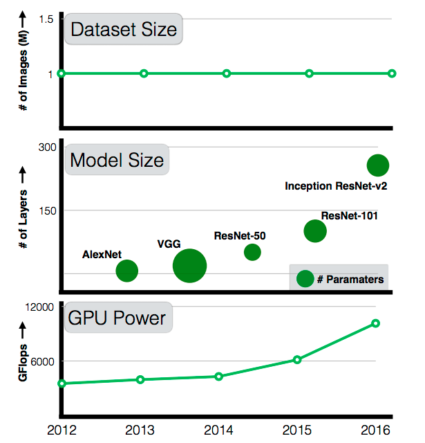
While GPU computation power and model sizes have continued to increase over the last five years, the size of the largest training dataset has surprisingly remained constant.
In our paper, “Revisiting Unreasonable Effectiveness of Data in Deep Learning Era”, we take the first steps towards clearing the clouds of mystery surrounding the relationship between `enormous data' and deep learning. Our goal was to explore: (a) if visual representations can be still improved by feeding more and more images with noisy labels to currently existing algorithms; (b) the nature of the relationship between data and performance on standard vision tasks such as classification, object detection and image segmentation; (c) state-of-the-art models for all the tasks in computer vision using large-scale learning.

Of course, the elephant in the room is where can we obtain a dataset that is 300x larger than ImageNet? At Google, we have been continuously working on building such datasets automatically to improve computer vision algorithms. Specifically, we have built an internal dataset of 300M images that are labeled with 18291 categories, which we call JFT-300M. The images are labeled using an algorithm that uses complex mixture of raw web signals, connections between web-pages and user feedback. This results in over one billion labels for the 300M images (a single image can have multiple labels). Of the billion image labels, approximately 375M are selected via an algorithm that aims to maximize label precision of selected images. However, there is still considerable noise in the labels: approximately 20% of the labels for selected images are noisy. Since there is no exhaustive annotation, we have no way to estimate the recall of the labels.

Our experimental results validate some of the hypotheses but also generate some unexpected surprises:
  • Better Representation Learning Helps. Our first observation is that large-scale data helps in representation learning which in-turn improves the performance on each vision task we study. Our findings suggest that a collective effort to build a large-scale dataset for pretraining is important. It also suggests a bright future for unsupervised and semi-supervised representation learning approaches. It seems the scale of data continues to overpower noise in the label space.
  • Performance increases linearly with orders of magnitude of training data.  Perhaps the most surprising finding is the relationship between performance on vision tasks and the amount of training data (log-scale) used for representation learning. We find that this relationship is still linear! Even at 300M training images, we do not observe any plateauing effect for the tasks studied.
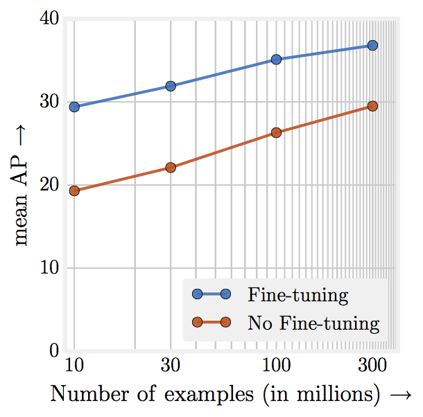
  • Object detection performance when pre-trained on different subsets of JFT-300M from scratch. x-axis is the dataset size in log-scale, y-axis is the detection performance in mAP@[.5,.95] on COCO-minival subset.
  • Capacity is Crucial. We also observe that to fully exploit 300M images, one needs higher capacity (deeper) models. For example, in case of ResNet-50 the gain on COCO object detection benchmark is much smaller (1.87%) compared to (3%) when using ResNet-152.
  • New state of the art results. Our paper presents new state-of-the-art results on several benchmarks using the models learned from JFT-300M. For example, a single model (without any bells and whistles) can now achieve 37.4 AP as compared to 34.3 AP on the COCO detection benchmark.
It is important to highlight that the training regime, learning schedules and parameters we used are based on our understanding of training ConvNets with 1M images from ImageNet. Since we do not search for the optimal set of hyper-parameters in this work (which would have required considerable computational effort), it is highly likely that these results are not the best ones you can obtain when using this scale of data. Therefore, we consider the quantitative performance reported to be an underestimate of the actual impact of data.

This work does not focus on task-specific data, such as exploring if more bounding boxes affects model performance. We believe that, although challenging, obtaining large scale task-specific data should be the focus of future study. Furthermore, building a dataset of 300M images should not be a final goal - as a community, we should explore if models continue to improve in the regime of even larger (1 billion+ image) datasets.

Core Contributors
Chen Sun, Abhinav Shrivastava, Saurabh Singh, and Abhinav Gupta

Acknowledgments
This work would not have been possible without the significant efforts of the Image Understanding and Expander teams at Google who built the massive JFT dataset. We would specifically like to thank Tom Duerig, Neil Alldrin, Howard Zhou, Lu Chen, David Cai, Gal Chechik, Zheyun Feng, Xiangxin Zhu and Rahul Sukthankar for their help. Also big thanks to the VALE team for APIs and specifically, Jonathan Huang, George Papandreou, Liang-Chieh Chen and Kevin Murphy for helpful discussions.

MobileNets: Open Source Models for Efficient On-Device Vision

Crossposted on the Google Research Blog

Deep learning has fueled tremendous progress in the field of computer vision in recent years, with neural networks repeatedly pushing the frontier of visual recognition technology. While many of those technologies such as object, landmark, logo and text recognition are provided for internet-connected devices through the Cloud Vision API, we believe that the ever-increasing computational power of mobile devices can enable the delivery of these technologies into the hands of our users, anytime, anywhere, regardless of internet connection. However, visual recognition for on device and embedded applications poses many challenges — models must run quickly with high accuracy in a resource-constrained environment making use of limited computation, power and space.

Today we are pleased to announce the release of MobileNets, a family of mobile-first computer vision models for TensorFlow, designed to effectively maximize accuracy while being mindful of the restricted resources for an on-device or embedded application. MobileNets are small, low-latency, low-power models parameterized to meet the resource constraints of a variety of use cases. They can be built upon for classification, detection, embeddings and segmentation similar to how other popular large scale models, such as Inception, are used.
Example use cases include detection, fine-grain classification, attributes and geo-localization.
This release contains the model definition for MobileNets in TensorFlow using TF-Slim, as well as 16 pre-trained ImageNet classification checkpoints for use in mobile projects of all sizes. The models can be run efficiently on mobile devices with TensorFlow Mobile.
Model Checkpoint
Million MACs
Million Parameters
Top-1 Accuracy
Top-5 Accuracy
569
4.24
70.7
89.5
418
4.24
69.3
88.9
291
4.24
67.2
87.5
186
4.24
64.1
85.3
317
2.59
68.4
88.2
233
2.59
67.4
87.3
162
2.59
65.2
86.1
104
2.59
61.8
83.6
150
1.34
64.0
85.4
110
1.34
62.1
84.0
77
1.34
59.9
82.5
49
1.34
56.2
79.6
41
0.47
50.6
75.0
34
0.47
49.0
73.6
21
0.47
46.0
70.7
14
0.47
41.3
66.2
Choose the right MobileNet model to fit your latency and size budget. The size of the network in memory and on disk is proportional to the number of parameters. The latency and power usage of the network scales with the number of Multiply-Accumulates (MACs) which measures the number of fused Multiplication and Addition operations. Top-1 and Top-5 accuracies are measured on the ILSVRC dataset.
We are excited to share MobileNets with the open source community. Information for getting started can be found at the TensorFlow-Slim Image Classification Library. To learn how to run models on-device please go to TensorFlow Mobile. You can read more about the technical details of MobileNets in our paper, MobileNets: Efficient Convolutional Neural Networks for Mobile Vision Applications.

By Andrew G. Howard, Senior Software Engineer and Menglong Zhu, Software Engineer

Acknowledgements
MobileNets were made possible with the hard work of many engineers and researchers throughout Google. Specifically we would like to thank:

Core Contributors: Andrew G. Howard, Menglong Zhu, Bo Chen, Dmitry Kalenichenko, Weijun Wang, Tobias Weyand, Marco Andreetto, Hartwig Adam

Special thanks to: Benoit Jacob, Skirmantas Kligys, George Papandreou, Liang-Chieh Chen, Derek Chow, Sergio Guadarrama, Jonathan Huang, Andre Hentz, Pete Warden

MobileNets: Open-Source Models for Efficient On-Device Vision


Deep learning has fueled tremendous progress in the field of computer vision in recent years, with neural networks repeatedly pushing the frontier of visual recognition technology. While many of those technologies such as object, landmark, logo and text recognition are provided for internet-connected devices through the Cloud Vision API, we believe that the ever-increasing computational power of mobile devices can enable the delivery of these technologies into the hands of our users, anytime, anywhere, regardless of internet connection. However, visual recognition for on device and embedded applications poses many challenges — models must run quickly with high accuracy in a resource-constrained environment making use of limited computation, power and space.

Today we are pleased to announce the release of MobileNets, a family of mobile-first computer vision models for TensorFlow, designed to effectively maximize accuracy while being mindful of the restricted resources for an on-device or embedded application. MobileNets are small, low-latency, low-power models parameterized to meet the resource constraints of a variety of use cases. They can be built upon for classification, detection, embeddings and segmentation similar to how other popular large scale models, such as Inception, are used.
Example use cases include detection, fine-grain classification, attributes and geo-localization.
This release contains the model definition for MobileNets in TensorFlow using TF-Slim, as well as 16 pre-trained ImageNet classification checkpoints for use in mobile projects of all sizes. The models can be run efficiently on mobile devices with TensorFlow Mobile.

Model Checkpoint
Million MACs
Million Parameters
Top-1 Accuracy
Top-5 Accuracy
569
4.24
70.7
89.5
418
4.24
69.3
88.9
291
4.24
67.2
87.5
186
4.24
64.1
85.3
317
2.59
68.4
88.2
233
2.59
67.4
87.3
162
2.59
65.2
86.1
104
2.59
61.8
83.6
150
1.34
64.0
85.4
110
1.34
62.1
84.0
77
1.34
59.9
82.5
49
1.34
56.2
79.6
41
0.47
50.6
75.0
34
0.47
49.0
73.6
21
0.47
46.0
70.7
14
0.47
41.3
66.2
Choose the right MobileNet model to fit your latency and size budget. The size of the network in memory and on disk is proportional to the number of parameters. The latency and power usage of the network scales with the number of Multiply-Accumulates (MACs) which measures the number of fused Multiplication and Addition operations. Top-1 and Top-5 accuracies are measured on the ILSVRC dataset.
We are excited to share MobileNets with the open-source community. Information for getting started can be found at the TensorFlow-Slim Image Classification Library. To learn how to run models on-device please go to TensorFlow Mobile. You can read more about the technical details of MobileNets in our paper, MobileNets: Efficient Convolutional Neural Networks for Mobile Vision Applications.

Acknowledgements
MobileNets were made possible with the hard work of many engineers and researchers throughout Google. Specifically we would like to thank:

Core Contributors: Andrew G. Howard, Menglong Zhu, Bo Chen, Dmitry Kalenichenko, Weijun Wang, Tobias Weyand, Marco Andreetto, Hartwig Adam

Special thanks to: Benoit Jacob, Skirmantas Kligys, George Papandreou, Liang-Chieh Chen, Derek Chow, Sergio Guadarrama, Jonathan Huang, Andre Hentz, Pete Warden

The Machine Intelligence Behind Gboard


Most people spend a significant amount of time each day using mobile-device keyboards: composing emails, texting, engaging in social media, and more. Yet, mobile keyboards are still cumbersome to handle. The average user is roughly 35% slower typing on a mobile device than on a physical keyboard. To change that, we recently provided many exciting improvements to Gboard for Android, working towards our vision of creating an intelligent mechanism that enables faster input while offering suggestions and correcting mistakes, in any language you choose.

With the realization that the way a mobile keyboard translates touch inputs into text is similar to how a speech recognition system translates voice inputs into text, we leveraged our experience in Speech Recognition to pursue our vision. First, we created robust spatial models that map fuzzy sequences of raw touch points to keys on the keyboard, just like acoustic models map sequences of sound bites to phonetic units. Second, we built a powerful core decoding engine based on finite state transducers (FST) to determine the likeliest word sequence given an input touch sequence. With its mathematical formalism and broad success in speech applications, we knew that an FST decoder would offer the flexibility needed to support a variety of complex keyboard input behaviors as well as language features. In this post, we will detail what went into the development of both of these systems.

Neural Spatial Models
Mobile keyboard input is subject to errors that are generally attributed to “fat finger typing” (or tracing spatially similar words in glide typing, as illustrated below) along with cognitive and motor errors (manifesting in misspellings, character insertions, deletions or swaps, etc). An intelligent keyboard needs to be able to account for these errors and predict the intended words rapidly and accurately. As such, we built a spatial model for Gboard that addresses these errors at the character level, mapping the touch points on the screen to actual keys.
Average glide trails for two spatially-similar words: “Vampire” and “Value”.
Up to recently, Gboard used a Gaussian model to quantify the probability of tapping neighboring keys and a rule-based model to represent cognitive and motor errors. These models were simple and intuitive, but they didn’t allow us to directly optimize metrics that correlate with better typing quality. Drawing on our experience with Voice Search acoustic models we replaced both the Gaussian and rule-based models with a single, highly efficient long short-term memory (LSTM) model trained with a connectionist temporal classification (CTC) criterion.

However, training this model turned out to be a lot more complicated than we had anticipated. While acoustic models are trained from human-transcribed audio data, one cannot easily transcribe millions of touch point sequences and glide traces. So the team exploited user-interaction signals, e.g. reverted auto-corrections and suggestion picks as negative and positive semi-supervised learning signals, to form rich training and test sets.
Raw data points corresponding to the word “could” (left), and normalized sampled trajectory with per-sample variances (right).
A plethora of techniques from the speech recognition literature was used to iterate on the NSM models to make them small and fast enough to be run on any device. The TensorFlow infrastructure was used to train hundreds of models, optimizing various signals surfaced by the keyboard: completions, suggestions, gliding, etc. After more than a year of work, the resulting models were about 6 times faster and 10 times smaller than the initial versions, they also showed about 15% reduction in bad autocorrects and 10% reduction in wrongly decoded gestures on offline datasets.

Finite-State Transducers
While the NSM uses spatial information to help determine what was tapped or swiped, there are additional constraints — lexical and grammatical — that can be brought to bear. A lexicon tells us what words occur in a language and a probabilistic grammar tells us what words are likely to follow other words. To encode this information we use finite-state transducers. FSTs have long been a key component of Google’s speech recognition and synthesis systems. They provide a principled way to represent various probabilistic models (lexicons, grammars, normalizers, etc) used in natural language processing together with the mathematical framework needed to manipulate, optimize, combine and search the models*.

In Gboard, a key-to-word transducer compactly represents the keyboard lexicon as shown in the figure below. It encodes the mapping from key sequences to words, allowing for alternative key sequences and optional spaces.
This transducer encodes “I”, “I’ve”, “If” along paths from the start state (the bold circle 1) to final states (the double circle states 0 and 1). Each arc is labeled with an input key (before the “:”) and a corresponding output word (after the “:”) where ε encodes the empty symbol. The apostrophe in “I’ve” can be omitted. The user may skip the space bar sometimes. To account for that, the space key transition between words in the transducer is optional. The ε and space back arcs allow accepting more than one word.
A probabilistic n-gram transducer is used to represent the language model for the keyboard. A state in the model represents an (up to) n-1 word context and an arc leaving that state is labeled with a successor word together with its probability of following that context (estimated from textual data). These, together with the spatial model that gives the likelihoods of sequences of key touches (discrete tap entries or continuous gestures in glide typing), are combined and explored with a beam search.

Generic FST principles, such as streaming, support for dynamic models, etc took us a long way towards building a new keyboard decoder, but several new functionalities also had to be added. When you speak, you don’t need the decoder to complete your words or guess what you will say next to save you a few syllables; but when you type, you appreciate the help of word completions and predictions. Also, we wanted the keyboard to provide seamless multilingual support, as shown below.
Trilingual input typing in Gboard.
It was a complex effort to get our new decoder off the ground, but the principled nature of FSTs has many benefits. For example, supporting transliterations for languages like Hindi is just a simple extension of the generic decoder.

Transliteration Models
In many languages with complex scripts, romanization systems have been developed to map characters into the Latin alphabet, often according to their phonetic pronunciations. For example, the Pinyin “xièxiè” corresponds to the Chinese characters “谢谢” (“thank you”). A Pinyin keyboard allows users to conveniently type words on a QWERTY layout and have them automatically “translated” into the target script. Likewise, a transliterated Hindi keyboard allows users to type “daanth” for “दांत” (teeth). Whereas Pinyin is an agreed-upon romanization system, Hindi transliterations are more fuzzy; for example “daant” would be a valid alternative for “दांत”.
Transliterated glide input for Hindi.
Just as we have a transducer mapping from letter sequences to words (a lexicon) and a weighted language model automaton providing probabilities for word sequences, we built weighted transducer mappings between Latin key sequences and target script symbol sequences for 22 Indic languages. Some languages have multiple writing systems (Bodo for example can be written in the Bengali or Devanagari scripts) so between transliterated and native layouts, we built 57 new input methods in just a few months.

The general nature of the FST decoder let us leverage all the work we had done to support completions, predictions, glide typing and many UI features with no extra effort, allowing us to offer a rich experience to our Indian users right from the start.

A More Intelligent Keyboard
All in all, our recent work cut the decoding latency by 50%, reduced the fraction of words users have to manually correct by more than 10%, allowed us to launch transliteration support for the 22 official languages of India, and enabled many new features you may have noticed.

While we hope that these recent changes improve your typing experience, we recognize that on-device typing is by no means solved. Gboard can still make suggestions that seem nonintuitive or of low utility and gestures can still be decoded to words a human would never pick. However, our shift towards powerful machine intelligence algorithms has opened new spaces that we’re actively exploring to make more useful tools and products for our users worldwide.

Acknowledgments
This work was done by Cyril Allauzen, Ouais Alsharif, Lars Hellsten, Tom Ouyang, Brian Roark and David Rybach, with help from Speech Data Operation team. Special thanks go to Johan Schalkwyk and Corinna Cortes for their support.


* The toolbox of relevant algorithms is available in the OpenFst open-source library.

Announcing TensorFlow 1.0


In just its first year, TensorFlow has helped researchers, engineers, artists, students, and many others make progress with everything from language translation to early detection of skin cancer and preventing blindness in diabetics. We’re excited to see people using TensorFlow in over 6000 open-source repositories online.

Today, as part of the first annual TensorFlow Developer Summit, hosted in Mountain View and livestreamed around the world, we’re announcing TensorFlow 1.0:

It’s faster: TensorFlow 1.0 is incredibly fast! XLA lays the groundwork for even more performance improvements in the future, and tensorflow.org now includes tips & tricks for tuning your models to achieve maximum speed. We’ll soon publish updated implementations of several popular models to show how to take full advantage of TensorFlow 1.0 - including a 7.3x speedup on 8 GPUs for Inception v3 and 58x speedup for distributed Inception v3 training on 64 GPUs!

It’s more flexible: TensorFlow 1.0 introduces a high-level API for TensorFlow, with tf.layers, tf.metrics, and tf.losses modules. We’ve also announced the inclusion of a new tf.keras module that provides full compatibility with Keras, another popular high-level neural networks library.

It’s more production-ready than ever: TensorFlow 1.0 promises Python API stability (details here), making it easier to pick up new features without worrying about breaking your existing code.

Other highlights from TensorFlow 1.0:
  • Python APIs have been changed to resemble NumPy more closely. For this and other backwards-incompatible changes made to support API stability going forward, please use our handy migration guide and conversion script.
  • Experimental APIs for Java and Go
  • Higher-level API modules tf.layers, tf.metrics, and tf.losses - brought over from tf.contrib.learn after incorporating skflow and TF Slim
  • Experimental release of XLA, a domain-specific compiler for TensorFlow graphs, that targets CPUs and GPUs. XLA is rapidly evolving - expect to see more progress in upcoming releases.
  • Introduction of the TensorFlow Debugger (tfdbg), a command-line interface and API for debugging live TensorFlow programs.
  • New Android demos for object detection and localization, and camera-based image stylization.
  • Installation improvements: Python 3 docker images have been added, and TensorFlow’s pip packages are now PyPI compliant. This means TensorFlow can now be installed with a simple invocation of pip install tensorflow.
We’re thrilled to see the pace of development in the TensorFlow community around the world. To hear more about TensorFlow 1.0 and how it’s being used, you can watch the TensorFlow Developer Summit talks on YouTube, covering recent updates from higher-level APIs to TensorFlow on mobile to our new XLA compiler, as well as the exciting ways that TensorFlow is being used:


Click here for a link to the livestream and video playlist (individual talks will be posted online later in the day).

The TensorFlow ecosystem continues to grow with new techniques like Fold for dynamic batching and tools like the Embedding Projector along with updates to our existing tools like TensorFlow Serving. We’re incredibly grateful to the community of contributors, educators, and researchers who have made advances in deep learning available to everyone. We look forward to working with you on forums like GitHub issues, Stack Overflow, @TensorFlow, the [email protected] group and at future events.

App Discovery With Google Play, Part 1: Understanding Topics


Every month, more than a billion users come to Google Play to download apps for their mobile devices. While some are looking for specific apps, like Snapchat, others come with only a broad notion of what they are interested in, like “horror games” or “selfie apps”. These broad searches by topic represent nearly half of the queries in Play Store, so it’s critical to find the most relevant apps.

Searches by topic require more than simply indexing apps by query terms; they require an understanding of the topics associated with an app. Machine learning approaches have been applied to similar problems, but success heavily depends on the number of training examples to learn about a topic. While for some popular topics such as “social networking” we had many labeled apps to learn from, the majority of topics had only a handful of examples. Our challenge was to learn from a very limited number of training examples and scale to millions of apps across thousands of topics, forcing us to adapt our machine learning techniques.

Our initial attempt was to build a deep neural network (DNN) trained to predict topics for an app based on words and phrases from the app title and description. For example, if the app description mentioned “frightening”, “very scary”, and “fear” then associate the “horror game” topic with it. However, given the learning capacity of DNNs, it completely “memorized” the topics for the apps in our small training data and failed to generalize to new apps it hadn’t seen before.

To generalize effectively, we needed a much larger dataset to train on, so we turned to how people learn as inspiration. In contrast to DNNs, human beings need much less training data. For example, you would likely need to see very few “horror game” app descriptions before learning how to generalize and associate new apps to that genre. Just by knowing the language describing the apps, people can correctly infer topics from even a few examples.

To emulate this, we tried a very rough approximation of this language-centric learning. We trained a neural network to learn how language was used to describe apps. We built a Skip-gram model, where the neural network attempts to predict the words around a given word, for example “share” given “photo”. The neural network encodes its knowledge as vectors of floating point numbers, referred to as embeddings. These embeddings were used to train another model called a classifier, capable of distinguishing which topics applied to an app. We now needed much less training data to learn about app topics, due to the large amount of learning already done with Skip-gram.

While this architecture generalized well for popular topics like “social networking”, we ran into a new problem for more niche topics like “selfie”. The single classifier built to predict all the topics together focused most of its learning on the popular topics, ignoring the errors it made on the less common ones. To solve this problem we built a separate classifier for each topic and tuned them in isolation.

This architecture produced reasonable results, but would still sometimes overgeneralize. For instance, it might associate Facebook with “dating” or Plants vs Zombies with “educational games”. To produce more precise classifiers, we needed higher volume and quality of training data. We treated the system described above as a coarse classifier that pruned down every possible {app, topic} pair, numbering in billions, to a more manageable list of {app, topic} pairs of interest. We built a pipeline to have human raters evaluate the classifier output and fed consensus results back as training data. This process allowed us to bootstrap from our existing system, giving us a path to steadily improve classifier performance.


To evaluate {app, topic} pairs by human raters, we asked them questions of the form, “To what extent is topic X related to app Y?” Multiple raters received the same question and independently selected answers on a rating scale to indicate if the topic was “important” for the app, “somewhat related”, or completely “off-topic”. Our initial evaluations showed a high level of disagreement amongst the raters. Diving deeper, we identified several causes of disagreement: vague guidelines for answer selection, insufficient rater training, evaluating broad topics like “computer files” and “game physics” that applied to most apps or games. Tackling these issues led to significant gains in rater agreement. Asking raters to choose an explicit reason for their answer from a curated list further improved reliability. Despite the improvements, we sometimes still have to “agree to disagree” and currently discard answers where raters fail to reach consensus.

These app topic classifiers enable search and discovery features in the Google Play Apps store. The current system helps provide relevant results to our users, but we are constantly exploring new ways to improve the system, through additional signals, architectural improvements and new algorithms. In Part 2 of this series, we will discuss how to personalize the app discovery experience for users.

Acknowledgments
This work was done within the Google Play team in close collaboration with Liadan O'Callaghan, Yuhua Zhu, Mark Taylor and Michael Watson.


Supercharging Style Transfer


Pastiche. A French word, it designates a work of art that imitates the style of another one (not to be confused with its more humorous Greek cousin, parody). Although it has been used for a long time in visual art, music and literature, pastiche has been getting mass attention lately with online forums dedicated to images that have been modified to be in the style of famous paintings. Using a technique known as style transfer, these images are generated by phone or web apps that allow a user to render their favorite picture in the style of a well known work of art.

Although users have already produced gorgeous pastiches using the current technology, we feel that it could be made even more engaging. Right now, each painting is its own island, so to speak: the user provides a content image, selects an artistic style and gets a pastiche back. But what if one could combine many different styles, exploring unique mixtures of well known artists to create an entirely unique pastiche?

Learning a representation for artistic style

In our recent paper titled “A Learned Representation for Artistic Style”, we introduce a simple method to allow a single deep convolutional style transfer network to learn multiple styles at the same time. The network, having learned multiple styles, is able to do style interpolation, where the pastiche varies smoothly from one style to another. Our method enables style interpolation in real-time as well, allowing this to be applied not only to static images, but also videos.
Credit: awesome dog role played by Google Brain team office dog Picabo.
In the video above, multiple styles are combined in real-time and the resulting style is applied using a single style transfer network. The user is provided with a set of 13 different painting styles and adjusts their relative strengths in the final style via sliders. In this demonstration, the user is an active participant in producing the pastiche.

A Quick History of Style Transfer

While transferring the style of one image to another has existed for nearly 15 years [1] [2], leveraging neural networks to accomplish it is both very recent and very fascinating. In “A Neural Algorithm of Artistic Style” [3], researchers Gatys, Ecker & Bethge introduced a method that uses deep convolutional neural network (CNN) classifiers. The pastiche image is found via optimization: the algorithm looks for an image which elicits the same kind of activations in the CNN’s lower layers - which capture the overall rough aesthetic of the style input (broad brushstrokes, cubist patterns, etc.) - yet produces activations in the higher layers - which capture the things that make the subject recognizable - that are close to those produced by the content image. From some starting point (e.g. random noise, or the content image itself), the pastiche image is progressively refined until these requirements are met.
Content image: The Tübingen Neckarfront by Andreas Praefcke, Style painting: “Head of a Clown”, by Georges Rouault.
The pastiches produced via this algorithm look spectacular:
Figure adapted from L. Gatys et al. "A Neural Algorithm of Artistic Style" (2015). 
This work is considered a breakthrough in the field of deep learning research because it provided the first proof of concept for neural network-based style transfer. Unfortunately this method for stylizing an individual image is computationally demanding. For instance, in the first demos available on the web, one would upload a photo to a server, and then still have plenty of time to go grab a cup of coffee before a result was available.

This process was sped up significantly by subsequent research [4, 5] that recognized that this optimization problem may be recast as an image transformation problem, where one wishes to apply a single, fixed painting style to an arbitrary content image (e.g. a photograph). The problem can then be solved by teaching a feed-forward, deep convolutional neural network to alter a corpus of content images to match the style of a painting. The goal of the trained network is two-fold: maintain the content of the original image while matching the visual style of the painting.

The end result of this was that what once took a few minutes for a single static image, could now be run real time (e.g. applying style transfer to a live video). However, the increase in speed that allowed real-time style transfer came with a cost - a given style transfer network is tied to the style of a single painting, losing some flexibility of the original algorithm, which was not tied to any one style. This means that to build a style transfer system capable of modeling 100 paintings, one has to train and store 100 separate style transfer networks.

Our Contribution: Learning and Combining Multiple Styles

We started from the observation that many artists from the impressionist period employ similar brush stroke techniques and color palettes. Furthermore, painting by say, Monet, are even more visually similar.
Poppy Field (left) and Impression, Sunrise (right) by Claude Monet. Images from Wikipedia
We leveraged this observation in our training of a machine learning system. That is, we trained a single system that is able to capture and generalize across many Monet paintings or even a diverse array of artists across genres. The pastiches produced are qualitatively comparable to those produced in previous work, while originating from the same style transfer network.
Pastiches produced by our single network, trained on 32 varied styles. These pastiches are qualitatively equivalent to those created by single-style networks: Image Credit: (from top to bottom) content photographs by Andreas Praefcke, Rich Niewiroski Jr. and J.-H. Janßen, (from left to right) style paintings by William Glackens, Paul Signac, Georges Rouault, Edvard Munch and Vincent van Gogh.
The technique we developed is simple to implement and is not memory intensive. Furthermore, our network, trained on several artistic styles, permits arbitrary combining multiple painting styles in real-time, as shown in the video above. Here are four styles being combined in different proportions on a photograph of Tübingen:
Unlike previous approaches to fast style transfer, we feel that this method of modeling multiple styles at the same time opens the door to exciting new ways for users to interact with style transfer algorithms, not only allowing the freedom to create new styles based on the mixture of several others, but to do it in real-time. Stay tuned for a future post on the Magenta blog, in which we will describe the algorithm in more detail and release the TensorFlow source code to run this model and demo yourself. We also recommend that you check out Nat & Lo’s fantastic video explanation on the subject of style transfer.

References

[1] Efros, Alexei A., and William T. Freeman. Image quilting for texture synthesis and transfer (2001).

[2] Hertzmann, Aaron, Charles E. Jacobs, Nuria Oliver, Brian Curless, and David H. Salesin. Image analogies (2001).

[3] Gatys, Leon A., Alexander S. Ecker, and Matthias Bethge. A Neural Algorithm of Artistic Style (2015).

[4] Ulyanov, Dmitry, Vadim Lebedev, Andrea Vedaldi, and Victor Lempitsky. Texture Networks: Feed-forward Synthesis of Textures and Stylized Images (2016).

[5] Johnson, Justin, Alexandre Alahi, and Li Fei-Fei. Perceptual Losses for Real-Time Style Transfer and Super-Resolution (2016).


* This work was done during an internship with the Google Brain Team. Vincent is currently a Ph.D. candidate at MILA, Université de Montréal.


Image Compression with Neural Networks


Data compression is used nearly everywhere on the internet - the videos you watch online, the images you share, the music you listen to, even the blog you're reading right now. Compression techniques make sharing the content you want quick and efficient. Without data compression, the time and bandwidth costs for getting the information you need, when you need it, would be exorbitant!

In "Full Resolution Image Compression with Recurrent Neural Networks", we expand on our previous research on data compression using neural networks, exploring whether machine learning can provide better results for image compression like it has for image recognition and text summarization. Furthermore, we are releasing our compression model via TensorFlow so you can experiment with compressing your own images with our network.

We introduce an architecture that uses a new variant of the Gated Recurrent Unit (a type of RNN that allows units to save activations and process sequences) called Residual Gated Recurrent Unit (Residual GRU). Our Residual GRU combines existing GRUs with the residual connections introduced in "Deep Residual Learning for Image Recognition" to achieve significant image quality gains for a given compression rate. Instead of using a DCT to generate a new bit representation like many compression schemes in use today, we train two sets of neural networks - one to create the codes from the image (encoder) and another to create the image from the codes (decoder).

Our system works by iteratively refining a reconstruction of the original image, with both the encoder and decoder using Residual GRU layers so that additional information can pass from one iteration to the next. Each iteration adds more bits to the encoding, which allows for a higher quality reconstruction. Conceptually, the network operates as follows:
  1. The initial residual, R[0], corresponds to the original image I: R[0] = I.
  2. Set i=1 for to the first iteration.
  3. Iteration[i] takes R[i-1] as input and runs the encoder and binarizer to compress the image into B[i].
  4. Iteration[i] runs the decoder on B[i] to generate a reconstructed image P[i].
  5. The residual for Iteration[i] is calculated: R[i] = I - P[i].
  6. Set i=i+1 and go to Step 3 (up to the desired number of iterations).
The residual image represents how different the current version of the compressed image is from the original. This image is then given as input to the network with the goal of removing the compression errors from the next version of the compressed image. The compressed image is now represented by the concatenation of B[1] through B[N]. For larger values of N, the decoder gets more information on how to reduce the errors and generate a higher quality reconstruction of the original image.

To understand how this works, consider the following example of the first two iterations of the image compression network, shown in the figures below. We start with an image of a lighthouse. On the first pass through the network, the original image is given as an input (R[0] = I). P[1] is the reconstructed image. The difference between the original image and encoded image is the residual, R[1], which represents the error in the compression.
Left: Original image, I = R[0]. Center: Reconstructed image, P[1]. Right: the residual, R[1], which represents the error introduced by compression.
On the second pass through the network, R[1] is given as the network’s input (see figure below). A higher quality image P[2] is then created. So how does the system recreate such a good image (P[2], center panel below) from the residual R[1]? Because the model uses recurrent nodes with memory, the network saves information from each iteration that it can use in the next one. It learned something about the original image in Iteration[1] that is used along with R[1] to generate a better P[2] from B[2]. Lastly, a new residual, R[2] (right), is generated by subtracting P[2] from the original image. This time the residual is smaller since there are fewer differences between the reconstructed image, and what we started with.
The second pass through the network. Left: R[1] is given as input. Center: A higher quality reconstruction, P[2]. Right: A smaller residual R[2] is generated by subtracting P[2] from the original image.
At each further iteration, the network gains more information about the errors introduced by compression (which is captured by the residual image). If it can use that information to predict the residuals even a little bit, the result is a better reconstruction. Our models are able to make use of the extra bits up to a point. We see diminishing returns, and at some point the representational power of the network is exhausted.

To demonstrate file size and quality differences, we can take a photo of Vash, a Japanese Chin, and generate two compressed images, one JPEG and one Residual GRU. Both images target a perceptual similarity of 0.9 MS-SSIM, a perceptual quality metric that reaches 1.0 for identical images. The image generated by our learned model results in an file 25% smaller than JPEG.
Left: Original image (1419 KB PNG) at ~1.0 MS-SSIM. Center: JPEG (33 KB) at ~0.9 MS-SSIM. Right: Residual GRU (24 KB) at ~0.9 MS-SSIM. This is 25% smaller for a comparable image quality
Taking a look around his nose and mouth, we see that our method doesn’t have the magenta blocks and noise in the middle of the image as seen in JPEG. This is due to the blocking artifacts produced by JPEG, whereas our compression network works on the entire image at once. However, there's a tradeoff -- in our model the details of the whiskers and texture are lost, but the system shows great promise in reducing artifacts.
Left: Original. Center: JPEG. Right: Residual GRU.
While today’s commonly used codecs perform well, our work shows that using neural networks to compress images results in a compression scheme with higher quality and smaller file sizes. To learn more about the details of our research and a comparison of other recurrent architectures, check out our paper. Our future work will focus on even better compression quality and faster models, so stay tuned!

Chat Smarter with Allo


At Google, we are continuously building products powered by Machine Learning to delight our users and simplify their lives. Today, we are excited to talk about the technology behind Allo, a new smart messaging app that uses the power of neural networks and Google Search to make your text conversations easier and more productive.

Just like Smart Reply for Inbox, Allo understands the conversation history to generate a set of suggestions that the user will likely want to respond with. In addition to understanding the context of your conversation, Allo learns your individual style, so the responses are personalized for you.
How does it work?

About a year ago, we started exploring how we can make communication easier and more fun to use. The idea of Smart Reply for Allo came from my teammate Sushant Prakash who, along with Ori Gershony, led their teams to build this technology. We began by experimenting with neural network based model architectures which had proven to be successful for sequence prediction, including the encoder-decoder model used in Smart Reply for Inbox.

One challenge we faced was that response generation in online conversations have very strict latency requirements. To address this, Pavel Sountsov and Sushant came up with an innovative two-stage model that works as follows. First, a recurrent neural network looks at the conversation context one word at a time and encodes it in the hidden state of a long short term memory (LSTM). Below, we show an example with a context ‘Where are you?’. The context has three tokens, each of which is embedded into a continuous space and input to the LSTM. The LSTM state now encodes the context as a continuous vector. This vector is used to generate the response as a discretized semantic class.
Each semantic class is associated with a set of possible messages that belong to it. We use a second recurrent network to generate a specific message from that set. This network also converts the context into a hidden LSTM state but this time the hidden state is used to generate the full message of the reply one token at a time. For example, now the LSTM after seeing the context “Where are you?” generates the tokens in the response: “I’m at work”.
A beam search is used to efficiently select the top-N highest scoring responses from among the very large set of possible messages that a LSTM can generate. A snippet of the search space explored by such a beam-search technique is shown below.
As with any large-scale product, there were several engineering challenges we had to solve in generating a set of high-quality responses efficiently. For example, in spite of the two staged architecture, our first few networks were very slow and required about half a second to generate a response. This was obviously a deal breaker when we are talking about real time communication apps! So we had to evolve our neural network architecture further to reduce the latency to less than 200ms. We moved from using a softmax layer to a hierarchical softmax layer which traverses a tree of words instead of traversing a list of words thus making it more efficient.

Another interesting challenge we had to solve when generating predictions is controlling for message length. Sometimes none of the most probable responses are appropriate - if the model predicts too short a message, it might not be useful to the user, and if we predict something too long, it might not fit on the phone screen. We solved this by biasing the beam search to follow paths that lead to higher utility responses instead of favoring just the responses that are most probable. That way, we can efficiently generate appropriate length response predictions that are useful to our users.

Personalized for you

The best part about these suggestions is that over time they are personalized to you so that your individual style is reflected in your conversations. For example, if you often reply to “How are you?” with “Fine.” instead of “I am good.”, it will learn your preference and your future suggestions will take that into account. This was accomplished by incorporating a user's "style" as one of the features in a Neural Network that is used to predict the next word in a response, resulting in suggestions that are customized for your personality and individual preferences. The user's style is captured in a sequence of numbers that we call the user embedding. These embeddings can be generated as part of the regular model training, but this approach requires waiting for many days for training to be complete and it cannot handle more than a handful of millions of users. To solve this issue, Alon Shafrir implemented a L-BFGS based technique to generate user embeddings quickly and at scale. Now, you'll be able to enjoy personalized suggestions after only a short time of using Allo.

More than just English

The neural network model described above is language agnostic so building separate prediction models for each language works quite well. To make sure that responses for each language benefit from our semantic understanding of other languages, Sujith Ravi came up with a graph-based machine learning technique that can connect possible responses across languages. Dana Movshovitz-Attias and Peter Young applied this technique to build a graph that connects responses to incoming messages and to other responses that have similar word embeddings and syntactic relationships. It also connects responses with similar meaning across languages based on the machine translation models developed by our Translate team.

With this graph, we use semi-supervised learning, as described in this paper, to learn the semantic meaning of responses and determine which are the most useful clusters of possible responses. As a result, we can allow the LSTM to score many possible variants of each possible response meaning, allowing the personalization routines to select the best response for the user in the context of the conversation. This also helps enforce diversity as we can now pick the final set of responses from different semantic clusters.

Here’s an example of how the graph might look for a set of messages related to greetings:
Beyond Smart Reply

I am also very excited about the Google assistant in Allo with which you can converse and get information about anything that Google Search knows about. It understands your sentences and helps you accomplish tasks directly from the conversation. For example, the Google assistant can help you discover a restaurant and reserve a table from within the Allo app when chatting with your friends. This has been made possible because of the cutting-edge research in natural language understanding that we have been doing at Google. More details to follow soon!

These smart features will be part of the Android and iOS apps for Allo that will be available later this summer. We can’t wait for you to try and enjoy it!

We wish to acknowledge the hard work of the following in building Smart Reply:

Ryan Cassidy, Dave Citron, Ori Gershony, Max Gubin, Pranav Khaitan, Harini Krishnamurthy, Patrick McGregor, Dana Movshovitz-Attias, Sergey Nazarov, Hung Pham, Sushant Prakash, Vivek Ramavajjala, Sujith Ravi, Sunita Sarawagi, Alon Shafrir, Pavel Sountsov, Peter Young, Shu Zhang

Announcing SyntaxNet: The World’s Most Accurate Parser Goes Open Source


At Google, we spend a lot of time thinking about how computer systems can read and understand human language in order to process it in intelligent ways. Today, we are excited to share the fruits of our research with the broader community by releasing SyntaxNet, an open-source neural network framework implemented in TensorFlow that provides a foundation for Natural Language Understanding (NLU) systems. Our release includes all the code needed to train new SyntaxNet models on your own data, as well as Parsey McParseface, an English parser that we have trained for you and that you can use to analyze English text.

Parsey McParseface is built on powerful machine learning algorithms that learn to analyze the linguistic structure of language, and that can explain the functional role of each word in a given sentence. Because Parsey McParseface is the most accurate such model in the world, we hope that it will be useful to developers and researchers interested in automatic extraction of information, translation, and other core applications of NLU.

How does SyntaxNet work?

SyntaxNet is a framework for what’s known in academic circles as a syntactic parser, which is a key first component in many NLU systems. Given a sentence as input, it tags each word with a part-of-speech (POS) tag that describes the word's syntactic function, and it determines the syntactic relationships between words in the sentence, represented in the dependency parse tree. These syntactic relationships are directly related to the underlying meaning of the sentence in question. To take a very simple example, consider the following dependency tree for Alice saw Bob:


This structure encodes that Alice and Bob are nouns and saw is a verb. The main verb saw is the root of the sentence and Alice is the subject (nsubj) of saw, while Bob is its direct object (dobj). As expected, Parsey McParseface analyzes this sentence correctly, but also understands the following more complex example:


This structure again encodes the fact that Alice and Bob are the subject and object respectively of saw, in addition that Alice is modified by a relative clause with the verb reading, that saw is modified by the temporal modifier yesterday, and so on. The grammatical relationships encoded in dependency structures allow us to easily recover the answers to various questions, for example whom did Alice see?, who saw Bob?, what had Alice been reading about? or when did Alice see Bob?.

Why is Parsing So Hard For Computers to Get Right?

One of the main problems that makes parsing so challenging is that human languages show remarkable levels of ambiguity. It is not uncommon for moderate length sentences - say 20 or 30 words in length - to have hundreds, thousands, or even tens of thousands of possible syntactic structures. A natural language parser must somehow search through all of these alternatives, and find the most plausible structure given the context. As a very simple example, the sentence Alice drove down the street in her car has at least two possible dependency parses:


The first corresponds to the (correct) interpretation where Alice is driving in her car; the second corresponds to the (absurd, but possible) interpretation where the street is located in her car. The ambiguity arises because the preposition in can either modify drove or street; this example is an instance of what is called prepositional phrase attachment ambiguity.

Humans do a remarkable job of dealing with ambiguity, almost to the point where the problem is unnoticeable; the challenge is for computers to do the same. Multiple ambiguities such as these in longer sentences conspire to give a combinatorial explosion in the number of possible structures for a sentence. Usually the vast majority of these structures are wildly implausible, but are nevertheless possible and must be somehow discarded by a parser.

SyntaxNet applies neural networks to the ambiguity problem. An input sentence is processed from left to right, with dependencies between words being incrementally added as each word in the sentence is considered. At each point in processing many decisions may be possible—due to ambiguity—and a neural network gives scores for competing decisions based on their plausibility. For this reason, it is very important to use beam search in the model. Instead of simply taking the first-best decision at each point, multiple partial hypotheses are kept at each step, with hypotheses only being discarded when there are several other higher-ranked hypotheses under consideration. An example of a left-to-right sequence of decisions that produces a simple parse is shown below for the sentence I booked a ticket to Google.
Furthermore, as described in our paper, it is critical to tightly integrate learning and search in order to achieve the highest prediction accuracy. Parsey McParseface and other SyntaxNet models are some of the most complex networks that we have trained with the TensorFlow framework at Google. Given some data from the Google supported Universal Treebanks project, you can train a parsing model on your own machine.

So How Accurate is Parsey McParseface?

On a standard benchmark consisting of randomly drawn English newswire sentences (the 20 year old Penn Treebank), Parsey McParseface recovers individual dependencies between words with over 94% accuracy, beating our own previous state-of-the-art results, which were already better than any previous approach. While there are no explicit studies in the literature about human performance, we know from our in-house annotation projects that linguists trained for this task agree in 96-97% of the cases. This suggests that we are approaching human performance—but only on well-formed text. Sentences drawn from the web are a lot harder to analyze, as we learned from the Google WebTreebank (released in 2011). Parsey McParseface achieves just over 90% of parse accuracy on this dataset.

While the accuracy is not perfect, it’s certainly high enough to be useful in many applications. The major source of errors at this point are examples such as the prepositional phrase attachment ambiguity described above, which require real world knowledge (e.g. that a street is not likely to be located in a car) and deep contextual reasoning. Machine learning (and in particular, neural networks) have made significant progress in resolving these ambiguities. But our work is still cut out for us: we would like to develop methods that can learn world knowledge and enable equal understanding of natural language across all languages and contexts.

To get started, see the SyntaxNet code and download the Parsey McParseface parser model. Happy parsing from the main developers, Chris Alberti, David Weiss, Daniel Andor, Michael Collins & Slav Petrov.