Tag Archives: Neural Networks

Real-time Continuous Transcription with Live Transcribe


The World Health Organization (WHO) estimates that there are 466 million people globally that are deaf and hard of hearing. A crucial technology in empowering communication and inclusive access to the world's information to this population is automatic speech recognition (ASR), which enables computers to detect audible languages and transcribe them into text for reading. Google's ASR is behind automated captions in Youtube, presentations in Slides and also phone calls. However, while ASR has seen multiple improvements in the past couple of years, the deaf and hard of hearing still mainly rely on manual-transcription services like CART in the US, Palantypist in the UK, or STTR in other countries. These services can be prohibitively expensive and often require to be scheduled far in advance, diminishing the opportunities for the deaf and hard of hearing to participate in impromptu conversations as well as social occasions. We believe that technology can bridge this gap and empower this community.

Today, we're announcing Live Transcribe, a free Android service that makes real-world conversations more accessible by bringing the power of automatic captioning into everyday, conversational use. Powered by Google Cloud, Live Transcribe captions conversations in real-time, supporting over 70 languages and more than 80% of the world's population. You can launch it with a single tap from within any app, directly from the accessibility icon on the system tray.

Building Live Transcribe
Previous ASR-based transcription systems have generally required compute-intensive models, exhaustive user research and expensive access to connectivity, all which hinder the adoption of automated continuous transcription. To address these issues and ensure reasonably accurate real-time transcription, Live Transcribe combines the results of extensive user experience (UX) research with seamless and sustainable connectivity to speech processing servers. Furthermore, we needed to ensure that connectivity to these servers didn't cause our users excessive data usage.

Relying on cloud ASR provides us greater accuracy, but we wanted to reduce the network data consumption that Live Transcribe requires. To do this, we implemented an on-device neural network-based speech detector, built on our previous work with AudioSet. This network is an image-like model, similar to our published VGGish model, which detects speech and automatically manages network connections to the cloud ASR engine, minimizing data usage over long periods of use.

User Experience
To make Live Transcribe as intuitive as possible, we partnered with Gallaudet University to kickstart user experience research collaborations that would ensure core user needs were satisfied while maximizing the potential of our technologies. We considered several different modalities, computers, tablets, smartphones, and even small projectors, iterating ways to display auditory information and captions. In the end, we decided to focus on the smartphone form factor because of the sheer ubiquity of these devices and the increasing capabilities they have.

Once this was established, we needed to address another important issue: displaying transcription confidence. Traditionally considered to be helpful to the user, our research explored whether we actually needed to show word-level or phrase-level confidence.
Displaying confidence level of the transcription. Yellow is high confidence, green is medium and blue is low confidence. White is fresh text awaiting context before finalizing. On the left, the coloring is at a per-phrase level while on the right is at a per-word level.1 Research found them to be distracting to the user without providing conversational value.
Reinforcing previous UX research in this space, our research shows that a transcript is easiest to read when it is not layered with these signals. Instead, Live Transcribe focuses on better presentation of the text and supplementing it with other auditory signals besides speech.

Another useful UX signal is the noise level of their current environment. Known as the cocktail party problem, understanding a speaker in a noisy room is a major challenge for computers. To address this, we built an indicator that visualizes the volume of user speech relative to background noise. This also gives users instant feedback on how well the microphone is receiving the incoming speech from the speaker, allowing them to adjust the placement of the phone.
The loudness and noise indicator is made of two concentric circles. The inner brighter circle, indicating the noise floor, tells a deaf user how audibly noisy the current environment is. The outer circle shows how well the speaker’s voice is received.Together, the circles visually show the relative difference intuitively.
Future Work
Potential future improvements in mobile-based automatic speech transcription include on-device recognition, speaker-separation, and speech enhancement. Relying solely on transcription can have pitfalls that can lead to miscommunication. Our research with Gallaudet University shows that combining it with other auditory signals like speech detection and a loudness indicator, makes a tangibly meaningful change in communication options for our users.

Live Transcribe is now available in a staged rollout on the Play Store, and is pre-installed on all Pixel 3 devices with the latest update. Live Transcribe can then be enabled via the Accessibility Settings. You can also read more about it on The Keyword.

Acknowledgements
Live Transcribe was made by researchers Chet Gnegy, Dimitri Kanevsky, and Justin S. Paul in collaboration with Android Accessibility team members Brian Kemler, Thomas Lin, Alex Huang, Jacqueline Huang, Ben Chung, Richard Chang, I-ting Huang, Jessie Lin, Ausmus Chang, Weiwei Wei, Melissa Barnhart and Bingying Xia. We'd also like to thank our close partners from Gallaudet University, Christian Vogler, Norman Williams and Paula Tucker.


1 Eagle-eyed readers can see the phrase level confidence mode in use by Dr. Obeidat in the video above.


Source: Google AI Blog


Improving Search for the next 20 years

https://storage.googleapis.com/gweb-uniblog-publish-prod/images/BLR_-_Koshys_1_1.max-1000x1000.jpg
Growing up in India, there was one good library in my town that I had access to—run by the British Council.  It was modest by western standards, and I had to take two buses just to get there. But I was lucky, because for every child like me, there were many more who didn’t have access to the same information that I did. Access to information changed my life, bringing me to the U.S. to study computer science and opening up huge possibilities for me that would not have been available without the education I had.
Ben's library
The British Council Library in my hometown.


When Google started 20 years ago, our mission was to organize the world’s information and make it universally accessible and useful. That seemed like an incredibly ambitious mission at the time—even considering that in 1998 the web consisted of just 25 million pages (roughly the equivalent of books in a small library).
Fast forward to today, and now we index hundreds of billions of pages in our index—more information than all the libraries in the world could hold. We’ve grown to serve people all over the world, offering Search in more than 150 languages and over 190 countries.
Through all of this, we’ve remained grounded in our mission. In fact, providing greater access to information is as core to our work today as it was when we first started. And while almost everything has changed about technology and the information available to us, the core principles of Search have stayed the same.
  • First and foremost, we focus on the user. Whether you’re looking for recipes, studying for an exam, or finding information on where to vote, we’re focused on serving your information needs.
  • We strive to give you the most relevant, highest quality information as quickly as possible. This was true when Google started with the Page Rank algorithm—the foundational technology to Search. And it’s just as true today.
  • We see billions of queries every day, and 15 percent of queries are ones we’ve never seen before. Given this scale, the only way to provide Search effectively is through an algorithmic approach. This helps us not just solve all the queries we’ve seen yesterday, but also all the ones we can’t anticipate for tomorrow.
  • Finally, we rigorously test every change we make. A key part of this testing is the rater guidelines which define our goals in search, and which are publicly available for anyone to see. Every change to Search is evaluated by experimentation and by raters using these guidelines. Last year alone, we ran more than 200,000 experiments that resulted in 2,400+ changes to search. Search will serve you better today than it did yesterday, and even better tomorrow.
As Google marks our 20th anniversary, I wanted to share a first look at the next chapter of Search, and how we’re working to make information more accessible and useful for people everywhere. This next chapter is driven by three fundamental shifts in how we think about Search:
    Underpinning each of these are our advancements in AI, improving our ability to understand language in ways that weren’t possible when Google first started. This is incredibly exciting, because over 20 years ago when I studied neural nets at school, they didn’t actually work very well...at all!
    But we’ve now reached the point where neural networks can help us take a major leap forward from understanding words to understanding concepts. Neural embeddings, an approach developed in the field of neural networks, allow us to transform words to fuzzier representations of the underlying concepts, and then match the concepts in the query with the concepts in the document. We call this technique neural matching. This can enable us to address queries like: “why does my TV look strange?” to surface the most relevant results for that question, even if the exact words aren’t contained in the page. (By the way, it turns out the reason is called the soap opera effect).
    Finding the right information about my TV is helpful in the moment. But AI can have much more profound effects. Whether it’s predicting areas that might be affected in a flood, or helping you identify the best job opportunities for you, AI can dramatically improve our ability to make information more accessible and useful.
    I’ve worked on Search at Google since the early days of its existence. One of the things that keeps me so inspired about Search all these years is our mission and how timeless it is. Providing greater access to information is fundamental to what we do, and there are always more ways we can help people access the information they need. That’s what pushes us forward to continue to make Search better for our users. And that’s why our work here is never done.

    Posted by Ben Gomes, VP, Search, News and Assistant

    How Can Neural Network Similarity Help Us Understand Training and Generalization?


    In order to solve tasks, deep neural networks (DNNs) progressively transform input data into a sequence of complex representations (i.e., patterns of activations across individual neurons). Understanding these representations is critically important, not only for interpretability, but also so that we can more intelligently design machine learning systems. However, understanding these representations has proven quite difficult, especially when comparing representations across networks. In a previous post, we outlined the benefits of Canonical Correlation Analysis (CCA) as a tool for understanding and comparing the representations of convolutional neural networks (CNNs), showing that they converge in a bottom-up pattern, with early layers converging to their final representations before later layers over the course of training.

    In “Insights on Representational Similarity in Neural Networks with Canonical Correlation” we develop this work further to provide new insights into the representational similarity of CNNs, including differences between networks which memorize (e.g., networks which can only classify images they have seen before) from those which generalize (e.g., networks which can correctly classify previously unseen images). Importantly, we also extend this method to provide insights into the dynamics of recurrent neural networks (RNNs), a class of models that are particularly useful for sequential data, such as language. Comparing RNNs is difficult in many of the same ways as CNNs, but RNNs present the additional challenge that their representations change over the course of a sequence. This makes CCA, with its helpful invariances, an ideal tool for studying RNNs in addition to CNNs. As such, we have additionally open sourced the code used for applying CCA on neural networks with the hope that will help the research community better understand network dynamics.

    Representational Similarity of Memorizing and Generalizing CNNs
    Ultimately, a machine learning system is only useful if it can generalize to new situations it has never seen before. Understanding the factors which differentiate between networks that generalize and those that don’t is therefore essential, and may lead to new methods to improve generalization performance. To investigate whether representational similarity is predictive of generalization, we studied two types of CNNs:
    • generalizing networks: CNNs trained on data with unmodified, accurate labels and which learn solutions which generalize to novel data.
    • memorizing networks: CNNs trained on datasets with randomized labels such that they must memorize the training data and cannot, by definition, generalize (as in Zhang et al., 2017).
    We trained multiple instances of each network, differing only in the initial randomized values of the network weights and the order of the training data, and used a new weighted approach to calculate the CCA distance measure (see our paper for details) to compare the representations within each group of networks and between memorizing and generalizing networks.

    We found that groups of different generalizing networks consistently converged to more similar representations (especially in later layers) than groups of memorizing networks (see figure below). At the softmax, which denotes the network’s ultimate prediction, the CCA distance for each group of generalizing and memorizing networks decreases substantially, as the networks in each separate group make similar predictions.
    Groups of generalizing networks (blue) converge to more similar solutions than groups of memorizing networks (red). CCA distance was calculated between groups of networks trained on real CIFAR-10 labels (“Generalizing”) or randomized CIFAR-10 labels (“Memorizing”) and between pairs of memorizing and generalizing networks (“Inter”).
    Perhaps most surprisingly, in later hidden layers, the representational distance between any given pair of memorizing networks was about the same as the representational distance between a memorizing and generalizing network (“Inter” in the plot above), despite the fact that these networks were trained on data with entirely different labels. Intuitively, this result suggests that while there are many different ways to memorize the training data (resulting in greater CCA distances), there are fewer ways to learn generalizable solutions. In future work, we plan to explore whether this insight can be used to regularize networks to learn more generalizable solutions.

    Understanding the Training Dynamics of Recurrent Neural Networks
    So far, we have only applied CCA to CNNs trained on image data. However, CCA can also be applied to calculate representational similarity in RNNs, both over the course of training and over the course of a sequence. Applying CCA to RNNs, we first asked whether the RNNs exhibit the same bottom-up convergence pattern we observed in our previous work for CNNs. To test this, we measured the CCA distance between the representation at each layer of the RNN over the course of training with its final representation at the end of training. We found that the CCA distance for layers closer to the input dropped earlier in training than for deeper layers, demonstrating that, like CNNs, RNNs also converge in a bottom-up pattern (see figure below).
    Convergence dynamics for RNNs over the course of training exhibit bottom up convergence, as layers closer to the input converge to their final representations earlier in training than later layers. For example, layer 1 converges to its final representation earlier in training than layer 2 than layer 3 and so on. Epoch designates the number of times the model has seen the entire training set while different colors represent the convergence dynamics of different layers.
    Additional findings in our paper show that wider networks (e.g., networks with more neurons at each layer) converge to more similar solutions than narrow networks. We also found that trained networks with identical structures but different learning rates converge to distinct clusters with similar performance, but highly dissimilar representations. We also apply CCA to RNN dynamics over the course of a single sequence, rather than simply over the course of training, providing some initial insights into the various factors which influence RNN representations over time.

    Conclusions
    These findings reinforce the utility of analyzing and comparing DNN representations in order to provide insights into network function, generalization, and convergence. However, there are still many open questions: in future work, we hope to uncover which aspects of the representation are conserved across networks, both in CNNs and RNNs, and whether these insights can be used to improve network performance. We encourage others to try out the code used for the paper to investigate what CCA can tell us about other neural networks!

    Acknowledgements
    Special thanks to Samy Bengio, who is a co-author on this work. We also thank Martin Wattenberg, Jascha Sohl-Dickstein and Jon Kleinberg for helpful comments.

    Source: Google AI Blog


    MobileNetV2: The Next Generation of On-Device Computer Vision Networks


    Last year we introduced MobileNetV1, a family of general purpose computer vision neural networks designed with mobile devices in mind to support classification, detection and more. The ability to run deep networks on personal mobile devices improves user experience, offering anytime, anywhere access, with additional benefits for security, privacy, and energy consumption. As new applications emerge allowing users to interact with the real world in real time, so does the need for ever more efficient neural networks.

    Today, we are pleased to announce the availability of MobileNetV2 to power the next generation of mobile vision applications. MobileNetV2 is a significant improvement over MobileNetV1 and pushes the state of the art for mobile visual recognition including classification, object detection and semantic segmentation. MobileNetV2 is released as part of TensorFlow-Slim Image Classification Library, or you can start exploring MobileNetV2 right away in coLaboratory. Alternately, you can download the notebook and explore it locally using Jupyter. MobileNetV2 is also available as modules on TF-Hub, and pretrained checkpoints can be found on github.

    MobileNetV2 builds upon the ideas from MobileNetV1 [1], using depthwise separable convolution as efficient building blocks. However, V2 introduces two new features to the architecture: 1) linear bottlenecks between the layers, and 2) shortcut connections between the bottlenecks1. The basic structure is shown below.
    Overview of MobileNetV2 Architecture. Blue blocks represent composite convolutional building blocks as shown above.
    The intuition is that the bottlenecks encode the model’s intermediate inputs and outputs while the inner layer encapsulates the model’s ability to transform from lower-level concepts such as pixels to higher level descriptors such as image categories. Finally, as with traditional residual connections, shortcuts enable faster training and better accuracy. You can learn more about the technical details in our paper, “MobileNet V2: Inverted Residuals and Linear Bottlenecks”.

    How does it compare to the first generation of MobileNets?
    Overall, the MobileNetV2 models are faster for the same accuracy across the entire latency spectrum. In particular, the new models use 2x fewer operations, need 30% fewer parameters and are about 30-40% faster on a Google Pixel phone than MobileNetV1 models, all while achieving higher accuracy.
    MobileNetV2 improves speed (reduced latency) and increased ImageNet Top 1 accuracy
    MobileNetV2 is a very effective feature extractor for object detection and segmentation. For example, for detection when paired with the newly introduced SSDLite [2] the new model is about 35% faster with the same accuracy than MobileNetV1. We have open sourced the model under the Tensorflow Object Detection API [4].

    Model
    Params
    Multiply-Adds
    mAP
    Mobile CPU
    MobileNetV1 + SSDLite
    5.1M
    1.3B
    22.2%
    270ms
    4.3M
    0.8B
    22.1%
    200ms

    To enable on-device semantic segmentation, we employ MobileNetV2 as a feature extractor in a reduced form of DeepLabv3 [3], that was announced recently. On the semantic segmentation benchmark, PASCAL VOC 2012, our resulting model attains a similar performance as employing MobileNetV1 as feature extractor, but requires 5.3 times fewer parameters and 5.2 times fewer operations in terms of Multiply-Adds.

    Model
    Params
    Multiply-Adds
    mIOU
    MobileNetV1 + DeepLabV3
    11.15M
    14.25B
    75.29%
    2.11M
    2.75B
    75.32%

    As we have seen MobileNetV2 provides a very efficient mobile-oriented model that can be used as a base for many visual recognition tasks. We hope by sharing it with the broader academic and open-source community we can help to advance research and application development.

    Acknowledgements:
    We would like to acknowledge our core contributors Menglong Zhu, Andrey Zhmoginov and Liang-Chieh Chen. We also give special thanks to Bo Chen, Dmitry Kalenichenko, Skirmantas Kligys, Mathew Tang, Weijun Wang, Benoit Jacob, George Papandreou and Hartwig Adam.

    References
    1. MobileNets: Efficient Convolutional Neural Networks for Mobile Vision Applications, Howard AG, Zhu M, Chen B, Kalenichenko D, Wang W, Weyand T, Andreetto M, Adam H, arXiv:1704.04861, 2017.
    2. MobileNetV2: Inverted Residuals and Linear Bottlenecks, Sandler M, Howard A, Zhu M, Zhmoginov A, Chen LC. arXiv preprint. arXiv:1801.04381, 2018.
    3. Rethinking Atrous Convolution for Semantic Image Segmentation, Chen LC, Papandreou G, Schroff F, Adam H. arXiv:1706.05587, 2017.
    4. Speed/accuracy trade-offs for modern convolutional object detectors, Huang J, Rathod V, Sun C, Zhu M, Korattikara A, Fathi A, Fischer I, Wojna Z, Song Y, Guadarrama S, Murphy K, CVPR 2017.
    5. Deep Residual Learning for Image Recognition, He, Kaiming, Xiangyu Zhang, Shaoqing Ren, and Jian Sun. arXiv:1512.03385,2015


    1 The shortcut (also known as skip) connections, popularized by ResNets[5] are commonly used to connect the non-bottleneck layers. MobilenNetV2 inverts this notion and connects the bottlenecks directly.

    MobileNetV2: The Next Generation of On-Device Computer Vision Networks


    Last year we introduced MobileNetV1, a family of general purpose computer vision neural networks designed with mobile devices in mind to support classification, detection and more. The ability to run deep networks on personal mobile devices improves user experience, offering anytime, anywhere access, with additional benefits for security, privacy, and energy consumption. As new applications emerge allowing users to interact with the real world in real time, so does the need for ever more efficient neural networks.

    Today, we are pleased to announce the availability of MobileNetV2 to power the next generation of mobile vision applications. MobileNetV2 is a significant improvement over MobileNetV1 and pushes the state of the art for mobile visual recognition including classification, object detection and semantic segmentation. MobileNetV2 is released as part of TensorFlow-Slim Image Classification Library, or you can start exploring MobileNetV2 right away in Colaboratory. Alternately, you can download the notebook and explore it locally using Jupyter. MobileNetV2 is also available as modules on TF-Hub, and pretrained checkpoints can be found on github.

    MobileNetV2 builds upon the ideas from MobileNetV1 [1], using depthwise separable convolution as efficient building blocks. However, V2 introduces two new features to the architecture: 1) linear bottlenecks between the layers, and 2) shortcut connections between the bottlenecks1. The basic structure is shown below.
    Overview of MobileNetV2 Architecture. Blue blocks represent composite convolutional building blocks as shown above.
    The intuition is that the bottlenecks encode the model’s intermediate inputs and outputs while the inner layer encapsulates the model’s ability to transform from lower-level concepts such as pixels to higher level descriptors such as image categories. Finally, as with traditional residual connections, shortcuts enable faster training and better accuracy. You can learn more about the technical details in our paper, “MobileNet V2: Inverted Residuals and Linear Bottlenecks”.

    How does it compare to the first generation of MobileNets?
    Overall, the MobileNetV2 models are faster for the same accuracy across the entire latency spectrum. In particular, the new models use 2x fewer operations, need 30% fewer parameters and are about 30-40% faster on a Google Pixel phone than MobileNetV1 models, all while achieving higher accuracy.
    MobileNetV2 improves speed (reduced latency) and increased ImageNet Top 1 accuracy
    MobileNetV2 is a very effective feature extractor for object detection and segmentation. For example, for detection when paired with the newly introduced SSDLite [2] the new model is about 35% faster with the same accuracy than MobileNetV1. We have open sourced the model under the Tensorflow Object Detection API [4].

    Model
    Params
    Multiply-Adds
    mAP
    Mobile CPU
    MobileNetV1 + SSDLite
    5.1M
    1.3B
    22.2%
    270ms
    4.3M
    0.8B
    22.1%
    200ms

    To enable on-device semantic segmentation, we employ MobileNetV2 as a feature extractor in a reduced form of DeepLabv3 [3], that was announced recently. On the semantic segmentation benchmark, PASCAL VOC 2012, our resulting model attains a similar performance as employing MobileNetV1 as feature extractor, but requires 5.3 times fewer parameters and 5.2 times fewer operations in terms of Multiply-Adds.

    Model
    Params
    Multiply-Adds
    mIOU
    MobileNetV1 + DeepLabV3
    11.15M
    14.25B
    75.29%
    2.11M
    2.75B
    75.32%

    As we have seen MobileNetV2 provides a very efficient mobile-oriented model that can be used as a base for many visual recognition tasks. We hope by sharing it with the broader academic and open-source community we can help to advance research and application development.

    Acknowledgements:
    We would like to acknowledge our core contributors Menglong Zhu, Andrey Zhmoginov and Liang-Chieh Chen. We also give special thanks to Bo Chen, Dmitry Kalenichenko, Skirmantas Kligys, Mathew Tang, Weijun Wang, Benoit Jacob, George Papandreou, Zhichao Lu, Vivek Rathod, Jonathan Huang, Yukun Zhu, and Hartwig Adam.

    References
    1. MobileNets: Efficient Convolutional Neural Networks for Mobile Vision Applications, Howard AG, Zhu M, Chen B, Kalenichenko D, Wang W, Weyand T, Andreetto M, Adam H, arXiv:1704.04861, 2017.
    2. MobileNetV2: Inverted Residuals and Linear Bottlenecks, Sandler M, Howard A, Zhu M, Zhmoginov A, Chen LC. arXiv preprint. arXiv:1801.04381, 2018.
    3. Rethinking Atrous Convolution for Semantic Image Segmentation, Chen LC, Papandreou G, Schroff F, Adam H. arXiv:1706.05587, 2017.
    4. Speed/accuracy trade-offs for modern convolutional object detectors, Huang J, Rathod V, Sun C, Zhu M, Korattikara A, Fathi A, Fischer I, Wojna Z, Song Y, Guadarrama S, Murphy K, CVPR 2017.
    5. Deep Residual Learning for Image Recognition, He, Kaiming, Xiangyu Zhang, Shaoqing Ren, and Jian Sun. arXiv:1512.03385,2015


    1 The shortcut (also known as skip) connections, popularized by ResNets[5] are commonly used to connect the non-bottleneck layers. MobilenNetV2 inverts this notion and connects the bottlenecks directly.

    Source: Google AI Blog


    Semantic Image Segmentation with DeepLab in TensorFlow

    Cross-posted on the Google Research Blog.

    Semantic image segmentation, the task of assigning a semantic label, such as “road”, “sky”, “person”, “dog”, to every pixel in an image enables numerous new applications, such as the synthetic shallow depth-of-field effect shipped in the portrait mode of the Pixel 2 and Pixel 2 XL smartphones and mobile real-time video segmentation. Assigning these semantic labels requires pinpointing the outline of objects, and thus imposes much stricter localization accuracy requirements than other visual entity recognition tasks such as image-level classification or bounding box-level detection.


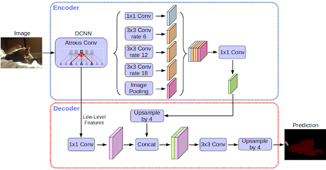
    Today, we are excited to announce the open source release of our latest and best performing semantic image segmentation model, DeepLab-v3+ [1]*, implemented in TensorFlow. This release includes DeepLab-v3+ models built on top of a powerful convolutional neural network (CNN) backbone architecture [2, 3] for the most accurate results, intended for server-side deployment. As part of this release, we are additionally sharing our TensorFlow model training and evaluation code, as well as models already pre-trained on the Pascal VOC 2012 and Cityscapes benchmark semantic segmentation tasks.

    Since the first incarnation of our DeepLab model [4] three years ago, improved CNN feature extractors, better object scale modeling, careful assimilation of contextual information, improved training procedures, and increasingly powerful hardware and software have led to improvements with DeepLab-v2 [5] and DeepLab-v3 [6]. With DeepLab-v3+, we extend DeepLab-v3 by adding a simple yet effective decoder module to refine the segmentation results especially along object boundaries. We further apply the depthwise separable convolution to both atrous spatial pyramid pooling [5, 6] and decoder modules, resulting in a faster and stronger encoder-decoder network for semantic segmentation.


    Modern semantic image segmentation systems built on top of convolutional neural networks (CNNs) have reached accuracy levels that were hard to imagine even five years ago, thanks to advances in methods, hardware, and datasets. We hope that publicly sharing our system with the community will make it easier for other groups in academia and industry to reproduce and further improve upon state-of-art systems, train models on new datasets, and envision new applications for this technology.

    By Liang-Chieh Chen and Yukun Zhu, Google Research

    Acknowledgements
    We would like to thank the support and valuable discussions with Iasonas Kokkinos, Kevin Murphy, Alan L. Yuille (co-authors of DeepLab-v1 and -v2), as well as Mark Sandler, Andrew Howard, Menglong Zhu, Chen Sun, Derek Chow, Andre Araujo, Haozhi Qi, Jifeng Dai, and the Google Mobile Vision team.

    References
    1. Encoder-Decoder with Atrous Separable Convolution for Semantic Image Segmentation, Liang-Chieh Chen, Yukun Zhu, George Papandreou, Florian Schroff, and Hartwig Adam, arXiv: 1802.02611, 2018.
    2. Xception: Deep Learning with Depthwise Separable Convolutions, François Chollet, Proc. of CVPR, 2017.
    3. Deformable Convolutional Networks — COCO Detection and Segmentation Challenge 2017 Entry, Haozhi Qi, Zheng Zhang, Bin Xiao, Han Hu, Bowen Cheng, Yichen Wei, and Jifeng Dai, ICCV COCO Challenge Workshop, 2017.
    4. Semantic Image Segmentation with Deep Convolutional Nets and Fully Connected CRFs, Liang-Chieh Chen, George Papandreou, Iasonas Kokkinos, Kevin Murphy, and Alan L. Yuille, Proc. of ICLR, 2015.
    5. Deeplab: Semantic Image Segmentation with Deep Convolutional Nets, Atrous Convolution, and Fully Connected CRFs, Liang-Chieh Chen, George Papandreou, Iasonas Kokkinos, Kevin Murphy, and Alan L. Yuille, TPAMI, 2017.
    6. Rethinking Atrous Convolution for Semantic Image Segmentation, Liang-Chieh Chen, George Papandreou, Florian Schroff, and Hartwig Adam, arXiv:1706.05587, 2017.


    * DeepLab-v3+ is not used to power Pixel 2's portrait mode or real time video segmentation. These are mentioned in the post as examples of features this type of technology can enable.

    Interpreting Deep Neural Networks with SVCCA


    Deep Neural Networks (DNNs) have driven unprecedented advances in areas such as vision, language understanding and speech recognition. But these successes also bring new challenges. In particular, contrary to many previous machine learning methods, DNNs can be susceptible to adversarial examples in classification, catastrophic forgetting of tasks in reinforcement learning, and mode collapse in generative modelling. In order to build better and more robust DNN-based systems, it is critically important to be able to interpret these models. In particular, we would like a notion of representational similarity for DNNs: can we effectively determine when the representations learned by two neural networks are same?

    In our paper, “SVCCA: Singular Vector Canonical Correlation Analysis for Deep Learning Dynamics and Interpretability,” we introduce a simple and scalable method to address these points. Two specific applications of this that we look at are comparing the representations learned by different networks, and interpreting representations learned by hidden layers in DNNs. Furthermore, we are open sourcing the code so that the research community can experiment with this method.

    Key to our setup is the interpretation of each neuron in a DNN as an activation vector. As shown in the figure below, the activation vector of a neuron is the scalar output it produces on the input data. For example, for 50 input images, a neuron in a DNN will output 50 scalar values, encoding how much it responds to each input. These 50 scalar values then make up an activation vector for the neuron. (Of course, in practice, we take many more than 50 inputs.)
    Here a DNN is given three inputs, x1, x2, x3. Looking at a neuron inside the DNN (bolded in red, right pane), this neuron produces a scalar output zi corresponding to each input xi. These values form the activation vector of the neuron.
    With this basic observation and a little more formulation, we introduce Singular Vector Canonical Correlation Analysis (SVCCA), a technique for taking in two sets of neurons and outputting aligned feature maps learned by both of them. Critically, this technique accounts for superficial differences such as permutations in neuron orderings (crucial for comparing different networks), and can detect similarities where other, more straightforward comparisons fail.

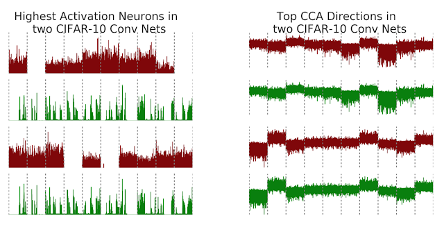
    As an example, consider training two convolutional neural nets (net1 and net2, below) on CIFAR-10, a medium scale image classification task. To visualize the results of our method, we compare activation vectors of neurons with the aligned features output by SVCCA. Recall that the activation vector of a neuron is the raw scalar outputs on input images. The x-axis of the plot consists of images sorted by class (gray dotted lines showing class boundaries), and the y axis the output value of the neuron.
    On the left pane, we show the two highest activation (largest euclidean norm) neurons in net1 and net2. Examining highest activations neurons has been a popular method to interpret DNNs in computer vision, but in this case, the highest activation neurons in net1 and net2 have no clear correspondence, despite both being trained on the same task. However, after applying SVCCA, (right pane), we see that the latent representations learned by both networks do indeed share some very similar features. Note that the top two rows representing aligned feature maps are close to identical, as are the second highest aligned feature maps (bottom two rows). Furthermore, these aligned mappings in the right pane also show a clear correspondence with the class boundaries, e.g. we see the top pair give negative outputs for Class 8, with the bottom pair giving a positive output for Class 2 and Class 7.

    While you can apply SVCCA across networks, one can also do this for the same network, across time, enabling the study of how different layers in a network converge to their final representations. Below, we show panes that compare the representation of layers in net1 during training (y-axes) with the layers at the end of training (x-axes). For example, in the top left pane (titled “0% trained”), the x-axis shows layers of increasing depth of net1 at 100% trained, and the y axis shows layers of increasing depth at 0% trained. Each (i,j) square then tells us how similar the representation of layer i at 100% trained is to layer j at 0% trained. The input layer is at the bottom left, and is (as expected) identical at 0% to 100%. We make this comparison at several points through training, at 0%, 35%, 75% and 100%, for convolutional (top row) and residual (bottom row) nets on CIFAR-10.
    Plots showing learning dynamics of convolutional and residual networks on CIFAR-10. Note the additional structure also visible: the 2x2 blocks in the top row are due to batch norm layers, and the checkered pattern in the bottom row due to residual connections.
    We find evidence of bottom-up convergence, with layers closer to the input converging first, and layers higher up taking longer to converge. This suggests a faster training method, Freeze Training — see our paper for details. Furthermore, this visualization also helps highlight properties of the network. In the top row, there are a couple of 2x2 blocks. These correspond to batch normalization layers, which are representationally identical to their previous layers. On the bottom row, towards the end of training, we can see a checkerboard like pattern appear, which is due to the residual connections of the network having greater similarity to previous layers.

    So far, we’ve concentrated on applying SVCCA to CIFAR-10. But applying preprocessing techniques with the Discrete Fourier transform, we can scale this method to Imagenet sized models. We applied this technique to the Imagenet Resnet, comparing the similarity of latent representations to representations corresponding to different classes:
    SVCCA similarity of latent representations with different classes. We take different layers in Imagenet Resnet, with 0 indicating input and 74 indicating output, and compare representational similarity of the hidden layer and the output class. Interestingly, different classes are learned at different speeds: the firetruck class is learned faster than the different dog breeds. Furthermore, the two pairs of dog breeds (a husky-like pair and a terrier-like pair) are learned at the same rate, reflecting the visual similarity between them.
    Our paper gives further details on the results we’ve explored so far, and also touches on different applications, e.g. compressing DNNs by projecting onto the SVCCA outputs, and Freeze Training, a computationally cheaper method for training deep networks. There are many followups we’re excited about exploring with SVCCA — moving on to different kinds of architectures, comparing across datasets, and better visualizing the aligned directions are just a few ideas we’re eager to try out. We look forward to presenting these results next week at NIPS 2017 in Long Beach, and we hope the code will also encourage many people to apply SVCCA to their network representations to interpret and understand what their network is learning.

    SLING: A Natural Language Frame Semantic Parser


    Until recently, most practical natural language understanding (NLU) systems used a pipeline of analysis stages, from part-of-speech tagging and dependency parsing to steps that computed a semantic representation of the input text. While this facilitated easy modularization of different analysis stages, errors in earlier stages would have cascading effects in later stages and the final representation, and the intermediate stage outputs might not be relevant on their own. For example, a typical pipeline might perform the task of dependency parsing in an early stage and the task of coreference resolution towards the end. If one was only interested in the output of coreference resolution, it would be affected by cascading effects of any errors during dependency parsing.

    Today we are announcing SLING, an experimental system for parsing natural language text directly into a representation of its meaning as a semantic frame graph. The output frame graph directly captures the semantic annotations of interest to the user, while avoiding the pitfalls of pipelined systems by not running any intermediate stages, additionally preventing unnecessary computation. SLING uses a special-purpose recurrent neural network model to compute the output representation of input text through incremental editing operations on the frame graph. The frame graph, in turn, is flexible enough to capture many semantic tasks of interest (more on this below). SLING's parser is trained using only the input words, bypassing the need for producing any intermediate annotations (e.g. dependency parses).

    SLING provides fast parsing at inference time by providing (a) an efficient and scalable frame store implementation and (b) a JIT compiler that generates efficient code to execute the recurrent neural network. Although SLING is experimental, it achieves a parsing speed of >2,500 tokens/second on a desktop CPU, thanks to its efficient frame store and neural network compiler. SLING is implemented in C++ and it is available for download on GitHub. The entire system is described in detail in a technical report as well.

    Frame Semantic Parsing
    Frame Semantics [1] represents the meaning of text — such as a sentence — as a set of formal statements. Each formal statement is called a frame, which can be seen as a unit of knowledge or meaning, that also contains interactions with concepts or other frames typically associated with it. SLING organizes each frame as a list of slots, where each slot has a name (role) and a value which could be a literal or a link to another frame. As an example, consider the sentence:

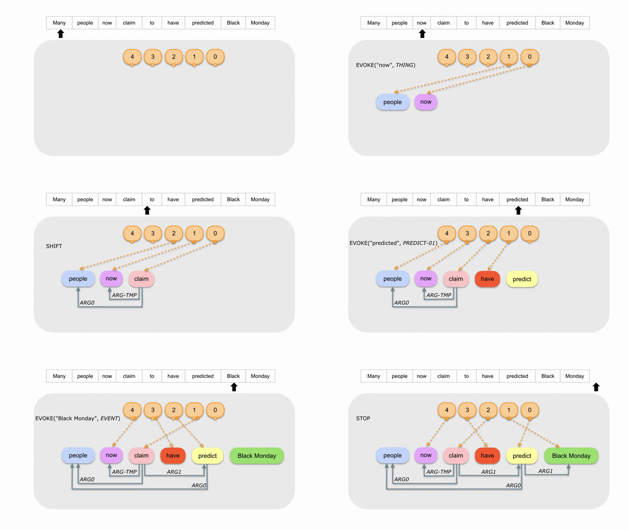
    “Many people now claim to have predicted Black Monday.”

    The figure below illustrates SLING recognizing mentions of entities (e.g. people, places, or events), measurements (e.g. dates or distances), and other concepts (e.g. verbs), and placing them in the correct semantic roles for the verbs in the input. The word predicted evokes the most dominant sense of the verb "predict", denoted as a PREDICT-01 frame. Additionally, this frame also has interactions (slots) with who made the prediction (denoted via the ARG0 slot, which points to the PERSON frame for people) and what was being predicted (denoted via ARG1, which links to the EVENT frame for Black Monday). Frame semantic parsing is the task of producing a directed graph of such frames linked through slots.
    Although the example above is fairly simple, frame graphs are powerful enough to model a variety of complex semantic annotation tasks. For starters, frames provide a convenient way to bring together language-internal and external information types (e.g. knowledge bases). This can then be used to address complex language understanding problems such as reference, metaphor, metonymy, and perspective. The frame graphs for these tasks only differ in the inventory of frame types, roles, and any linking constraints.

    SLING
    SLING trains a recurrent neural network by optimizing for the semantic frames of interest.
    The internal learned representations in the network’s hidden layers replace the hand-crafted feature combinations and intermediate representations in pipelined systems. Internally, SLING uses an encoder-decoder architecture where each input word is encoded into a vector using simple lexical features like the raw word, its suffix(es), punctuation etc. The decoder uses that representation, along with recurrent features from its own history, to compute a sequence of transitions that update the frame graph to obtain the intended frame semantic representation of the input sentence. SLING trains its model using TensorFlow and DRAGNN.

    The animation below shows how frames and roles are incrementally added to the under-construction frame graph using individual transitions. As discussed earlier with our simple example sentence, SLING connects the VERB and EVENT frames using the role ARG1, signifying that the EVENT frame is the concept being predicted. The EVOKE transition evokes a frame of a specified type from the next few tokens in the text (e.g. EVENT from Black Monday). Similarly, the CONNECT transition links two existing frames with a specified role. When the input is exhausted and the last transition (denoted as STOP) is executed, the frame graph is deemed as complete and returned to the user, who can inspect the graph to get the semantic meaning behind the sentence.
    One key aspect of our transition system is the presence of a small fixed-size attention buffer of frames that represents the most recent frames to be evoked or modified, shown with the orange boxes in the figure above. This buffer captures the intuition that we tend to remember knowledge that was recently evoked, referred to, or enhanced. If a frame is no longer in use, it eventually gets flushed out of this buffer as new frames come into picture. We found this simple mechanism to be surprisingly effective at capturing a large fraction of inter-frame links.

    Next Steps
    The illustrative experiment above is just a launchpad for research in semantic parsing for tasks such as knowledge extraction, resolving complex references, and dialog understanding. The SLING release on Github comes with a pre-trained model for the task we illustrated, as well as examples and recipes to train your own parser on either the supplied synthetic data or your own data. We hope the community finds SLING useful and we look forward to engaging conversations about applying and extending SLING to other semantic parsing tasks.

    Acknowledgements
    The research described in this post was done by Michael Ringgaard, Rahul Gupta, and Fernando Pereira. We thank the Tensorflow and DRAGNN teams for open-sourcing their packages, and various colleagues at DRAGNN who helped us with multiple aspects of SLING's training setup.


    1 Charles J. Fillmore. 1982. Frame semantics. Linguistics in the Morning Calm, pages 111–138.

    Building Your Own Neural Machine Translation System in TensorFlow


    Machine translation – the task of automatically translating between languages – is one of the most active research areas in the machine learning community. Among the many approaches to machine translation, sequence-to-sequence ("seq2seq") models [1, 2] have recently enjoyed great success and have become the de facto standard in most commercial translation systems, such as Google Translate, thanks to its ability to use deep neural networks to capture sentence meanings. However, while there is an abundance of material on seq2seq models such as OpenNMT or tf-seq2seq, there is a lack of material that teaches people both the knowledge and the skills to easily build high-quality translation systems.

    Today we are happy to announce a new Neural Machine Translation (NMT) tutorial for TensorFlow that gives readers a full understanding of seq2seq models and shows how to build a competitive translation model from scratch. The tutorial is aimed at making the process as simple as possible, starting with some background knowledge on NMT and walking through code details to build a vanilla system. It then dives into the attention mechanism [3, 4], a key ingredient that allows NMT systems to handle long sentences. Finally, the tutorial provides details on how to replicate key features in the Google’s NMT (GNMT) system [5] to train on multiple GPUs.

    The tutorial also contains detailed benchmark results, which users can replicate on their own. Our models provide a strong open-source baseline with performance on par with GNMT results [5]. We achieve 24.4 BLEU points on the popular WMT’14 English-German translation task.
    Other benchmark results (English-Vietnamese, German-English) can be found in the tutorial.

    In addition, this tutorial showcases the fully dynamic seq2seq API (released with TensorFlow 1.2) aimed at making building seq2seq models clean and easy:
    • Easily read and preprocess dynamically sized input sequences using the new input pipeline in tf.contrib.data.
    • Use padded batching and sequence length bucketing to improve training and inference speeds.
    • Train seq2seq models using popular architectures and training schedules, including several types of attention and scheduled sampling.
    • Perform inference in seq2seq models using in-graph beam search.
    • Optimize seq2seq models for multi-GPU settings.
    We hope this will help spur the creation of, and experimentation with, many new NMT models by the research community. To get started on your own research, check out the tutorial on GitHub!

    Core contributors
    Thang Luong, Eugene Brevdo, and Rui Zhao.

    Acknowledgements
    We would like to especially thank our collaborator on the NMT project, Rui Zhao. Without his tireless effort, this tutorial would not have been possible. Additional thanks go to Denny Britz, Anna Goldie, Derek Murray, and Cinjon Resnick for their work bringing new features to TensorFlow and the seq2seq library. Lastly, we thank Lukasz Kaiser for the initial help on the seq2seq codebase; Quoc Le for the suggestion to replicate GNMT; Yonghui Wu and Zhifeng Chen for details on the GNMT systems; as well as the Google Brain team for their support and feedback!

    References
    [1] Sequence to sequence learning with neural networks, Ilya Sutskever, Oriol Vinyals, and Quoc V. Le. NIPS, 2014.
    [2] Learning phrase representations using RNN encoder-decoder for statistical machine translation, Kyunghyun Cho, Bart Van Merrienboer, Caglar Gulcehre, Dzmitry Bahdanau, Fethi Bougares, Holger Schwenk, and Yoshua Bengio. EMNLP 2014.
    [3] Neural machine translation by jointly learning to align and translate, Dzmitry Bahdanau, Kyunghyun Cho, and Yoshua Bengio. ICLR, 2015.
    [4] Effective approaches to attention-based neural machine translation, Minh-Thang Luong, Hieu Pham, and Christopher D Manning. EMNLP, 2015.
    [5] Google’s Neural Machine Translation System: Bridging the Gap between Human and Machine Translation, Yonghui Wu, Mike Schuster, Zhifeng Chen, Quoc V. Le, Mohammad Norouzi, Wolfgang Macherey, Maxim Krikun, Yuan Cao, Qin Gao, Klaus Macherey, Jeff Klingner, Apurva Shah, Melvin Johnson, Xiaobing Liu, Łukasz Kaiser, Stephan Gouws, Yoshikiyo Kato, Taku Kudo, Hideto Kazawa, Keith Stevens, George Kurian, Nishant Patil, Wei Wang, Cliff Young, Jason Smith, Jason Riesa, Alex Rudnick, Oriol Vinyals, Greg Corrado, Macduff Hughes, Jeffrey Dean. Technical Report, 2016.