Tag Archives: Multimodal Learning

ALIGN: Scaling Up Visual and Vision-Language Representation Learning With Noisy Text Supervision

Learning good visual and vision-language representations is critical to solving computer vision problems — image retrieval, image classification, video understanding — and can enable the development of tools and products that change people’s daily lives. For example, a good vision-language matching model can help users find the most relevant images given a text description or an image input and help tools such as Google Lens find more fine-grained information about an image.

To learn such representations, current state-of-the-art (SotA) visual and vision-language models rely heavily on curated training datasets that require expert knowledge and extensive labels. For vision applications, representations are mostly learned on large-scale datasets with explicit class labels, such as ImageNet, OpenImages, and JFT-300M. For vision-language applications, popular pre-training datasets, such as Conceptual Captions and Visual Genome Dense Captions, all require non-trivial data collection and cleaning steps, limiting the size of datasets and thus hindering the scale of the trained models. In contrast, natural language processing (NLP) models have achieved SotA performance on GLUE and SuperGLUE benchmarks by utilizing large-scale pre-training on raw text without human labels.

In "Scaling Up Visual and Vision-Language Representation Learning With Noisy Text Supervision", to appear at ICML 2021, we propose bridging this gap with publicly available image alt-text data (written copy that appears in place of an image on a webpage if the image fails to load on a user's screen) in order to train larger, state-of-the-art vision and vision-language models. To that end, we leverage a noisy dataset of over one billion image and alt-text pairs, obtained without expensive filtering or post-processing steps in the Conceptual Captions dataset. We show that the scale of our corpus can make up for noisy data and leads to SotA representation, and achieves strong performance when transferred to classification tasks such as ImageNet and VTAB. The aligned visual and language representations also set new SotA results on Flickr30K and MS-COCO benchmarks, even when compared with more sophisticated cross-attention models, and enable zero-shot image classification and cross-modality search with complex text and text + image queries.

Creating the Dataset
Alt-texts usually provide a description of what the image is about, but the dataset is “noisy” because some text may be partly or wholly unrelated to its paired image.
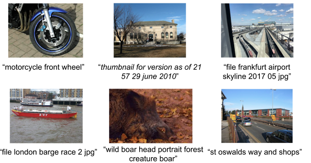
Example image-text pairs randomly sampled from the training dataset of ALIGN. One clearly noisy text label is marked in italics.

In this work, we follow the methodology of constructing the Conceptual Captions dataset to get a version of raw English alt-text data (image and alt-text pairs). While the Conceptual Captions dataset was cleaned by heavy filtering and post-processing, this work scales up visual and vision-language representation learning by relaxing most of the cleaning steps in the original work. Instead, we only apply minimal frequency-based filtering. The result is a much larger but noisier dataset of 1.8B image-text pairs.

ALIGN: A Large-scale ImaGe and Noisy-Text Embedding
For the purpose of building larger and more powerful models easily, we employ a simple dual-encoder architecture that learns to align visual and language representations of the image and text pairs. Image and text encoders are learned via a contrastive loss (formulated as normalized softmax) that pushes the embeddings of matched image-text pairs together while pushing those of non-matched image-text pairs (within the same batch) apart. The large-scale dataset makes it possible for us to scale up the model size to be as large as EfficientNet-L2 (image encoder) and BERT-large (text encoder) trained from scratch. The learned representation can be used for downstream visual and vision-language tasks.

Figure of ImageNet credit to (Krizhevsky et al. 2012) and VTAB figure credit to (Zhai et al. 2019)

The resulting representation can be used for vision-only or vision-language task transfer. Without any fine-tuning, ALIGN powers cross-modal search – image-to-text search, text-to-image search, and even search with joint image+text queries, examples below.

Evaluating Retrieval and Representation
The learned ALIGN model with BERT-Large and EfficientNet-L2 as text and image encoder backbones achieves SotA performance on multiple image-text retrieval tasks (Flickr30K and MS-COCO) in both zero-shot and fine-tuned settings, as shown below.

Flickr30K (1K test set) R@1 MS-COCO (5K test set) R@1
Setting Model    image → text       text → image       image → text       text → image   
Zero-shot ImageBERT    70.7 54.3 44.0 32.3
UNITER 83.6 68.7 - -
CLIP 88.0 68.7 58.4 37.8
ALIGN 88.6 75.7 58.6 45.6
Fine-tuned    GPO 88.7 76.1 68.1 52.7
UNITER 87.3 75.6 65.7 52.9
ERNIE-ViL 88.1 76.7 - -
VILLA 87.9 76.3 - -
Oscar - - 73.5 57.5
ALIGN 95.3 84.9 77.0 59.9
Image-text retrieval results (recall@1) on Flickr30K and MS-COCO datasets (both zero-shot and fine-tuned). ALIGN significantly outperforms existing methods including the cross-modality attention models that are too expensive for large-scale retrieval applications.

ALIGN is also a strong image representation model. Shown below, with frozen features, ALIGN slightly outperforms CLIP and achieves a SotA result of 85.5% top-1 accuracy on ImageNet. With fine-tuning, ALIGN achieves higher accuracy than most generalist models, such as BiT and ViT, and is only worse than Meta Pseudo Labels, which requires deeper interaction between ImageNet training and large-scale unlabeled data.

Model (backbone)    Acc@1 w/ frozen features       Acc@1       Acc@5   
WSL (ResNeXt-101 32x48d) 83.6 85.4 97.6
CLIP (ViT-L/14) 85.4 - -
BiT (ResNet152 x 4) - 87.54 98.46
NoisyStudent (EfficientNet-L2) - 88.4 98.7
ViT (ViT-H/14) - 88.55 -
Meta-Pseudo-Labels (EfficientNet-L2)    - 90.2 98.8
ALIGN (EfficientNet-L2) 85.5 88.64 98.67
ImageNet classification results comparison with supervised training (fine-tuning).

Zero-Shot Image Classification
Traditionally, image classification problems treat each class as independent IDs, and people have to train the classification layers with at least a few shots of labeled data per class. The class names are actually also natural language phrases, so we can naturally extend the image-text retrieval capability of ALIGN for image classification without any training data.

The pre-trained image and text encoder can directly be used in classifying an image into a set of classes by retrieving the nearest class name in the aligned embedding space. This approach does not require any training data for the defined class space.

On the ImageNet validation dataset, ALIGN achieves 76.4% top-1 zero-shot accuracy and shows great robustness in different variants of ImageNet with distribution shifts, similar to the concurrent work CLIP. We also use the same text prompt engineering and ensembling as in CLIP.

   ImageNet       ImageNet-R       ImageNet-A       ImageNet-V2   
CLIP 76.2 88.9 77.2 70.1
ALIGN    76.4 92.2 75.8 70.1
Top-1 accuracy of zero-shot classification on ImageNet and its variants.

Application in Image Search
To illustrate the quantitative results above, we build a simple image retrieval system with the embeddings trained by ALIGN and show the top 1 text-to-image retrieval results for a handful of text queries from a 160M image pool. ALIGN can retrieve precise images given detailed descriptions of a scene, or fine-grained or instance-level concepts like landmarks and artworks. These examples demonstrate that the ALIGN model can align images and texts with similar semantics, and that ALIGN can generalize to novel complex concepts.

Image retrieval with fine-grained text queries using ALIGN's embeddings.

Multimodal (Image+Text) Query for Image Search
A surprising property of word vectors is that word analogies can often be solved with vector arithmetic. A common example, "king – man + woman = queen". Such linear relationships between image and text embeddings also emerge in ALIGN.

Specifically, given a query image and a text string, we add their ALIGN embeddings together and use it to retrieve relevant images using cosine similarity, as shown below. These examples not only demonstrate the compositionality of ALIGN embeddings across vision and language domains, but also show the feasibility of searching with a multi-modal query. For instance, one could now look for the "Australia" or "Madagascar" equivalence of pandas, or turn a pair of black shoes into identically-looking beige shoes. Also, it is possible to remove objects/attributes from a scene by performing subtraction in the embedding space, shown below.

Image retrieval with image text queries. By adding or subtracting text query embedding, ALIGN retrieves relevant images.

Social Impact and Future Work
While this work shows promising results from a methodology perspective with a simple data collection method, additional analysis of the data and the resulting model is necessary before the responsible use of the model in practice. For instance, considerations should be made towards the potential for the use of harmful text data in alt-texts to reinforce such harms. With regard to fairness, data balancing efforts may be required to prevent reinforcing stereotypes from the web data. Additional testing and training around sensitive religious or cultural items should be taken to understand and mitigate the impact from possibly mislabeled data.

Further analysis should also be taken to ensure that the demographic distribution of humans and related cultural items, such as clothing, food, and art, do not cause skewed model performance. Analysis and balancing would be required if such models will be used in production.

Conclusion
We have presented a simple method of leveraging large-scale noisy image-text data to scale up visual and vision-language representation learning. The resulting model, ALIGN, is capable of cross-modal retrieval and significantly outperforms SotA models. In visual-only downstream tasks, ALIGN is also comparable to or outperforms SotA models trained with large-scale labeled data.

Acknowledgement
We would like to thank our co-authors in Google Research: Ye Xia, Yi-Ting Chen, Zarana Parekh, Hieu Pham, Quoc V. Le, Yunhsuan Sung, Zhen Li, Tom Duerig. This work was also done with invaluable help from other colleagues from Google. We would like to thank Jan Dlabal and Zhe Li for continuous support in training infrastructure, Simon Kornblith for building the zero-shot & robustness model evaluation on ImageNet variants, Xiaohua Zhai for help on conducting VTAB evaluation, Mingxing Tan and Max Moroz for suggestions on EfficientNet training, Aleksei Timofeev for the early idea of multimodal query retrieval, Aaron Michelony and Kaushal Patel for their early work on data generation, and Sergey Ioffe, Jason Baldridge and Krishna Srinivasan for the insightful feedback and discussion.

Source: Google AI Blog


Crisscrossed Captions: Semantic Similarity for Images and Text

The past decade has seen remarkable progress on automatic image captioning, a task in which a computer algorithm creates written descriptions for images. Much of the progress has come through the use of modern deep learning methods developed for both computer vision and natural language processing, combined with large scale datasets that pair images with descriptions created by people. In addition to supporting important practical applications, such as providing descriptions of images for visually impaired people, these datasets also enable investigations into important and exciting research questions about grounding language in visual inputs. For example, learning deep representations for a word like “car”, means using both linguistic and visual contexts.

Image captioning datasets that contain pairs of textual descriptions and their corresponding images, such as MS-COCO and Flickr30k, have been widely used to learn aligned image and text representations and to build captioning models. Unfortunately, these datasets have limited cross-modal associations: images are not paired with other images, captions are only paired with other captions of the same image (also called co-captions), there are image-caption pairs that match but are not labeled as a match, and there are no labels that indicate when an image-caption pair does not match. This undermines research into how inter-modality learning (connecting captions to images, for example) impacts intra-modality tasks (connecting captions to captions or images to images). This is important to address, especially because a fair amount of work on learning from images paired with text is motivated by arguments about how visual elements should inform and improve representations of language.

To address this evaluation gap, we present "Crisscrossed Captions: Extended Intramodal and Intermodal Semantic Similarity Judgments for MS-COCO", which was recently presented at EACL 2021. The Crisscrossed Captions (CxC) dataset extends the development and test splits of MS-COCO with semantic similarity ratings for image-text, text-text and image-image pairs. The rating criteria are based on Semantic Textual Similarity, an existing and widely-adopted measure of semantic relatedness between pairs of short texts, which we extend to include judgments about images as well. In all, CxC contains human-derived semantic similarity ratings for 267,095 pairs (derived from 1,335,475 independent judgments), a massive extension in scale and detail to the 50k original binary pairings in MS-COCO’s development and test splits. We have released CxC’s ratings, along with code to merge CxC with existing MS-COCO data. Anyone familiar with MS-COCO can thus easily enhance their experiments with CxC.

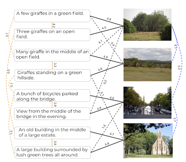
Crisscrossed Captions extends the MS-COCO evaluation sets by adding human-derived semantic similarity ratings for existing image-caption pairs and co-captions (solid lines), and it increases rating density by adding human ratings for new image-caption, caption-caption and image-image pairs (dashed lines).*

Creating the CxC Dataset
If a picture is worth a thousand words, it is likely because there are so many details and relationships between objects that are generally depicted in pictures. We can describe the texture of the fur on a dog, name the logo on the frisbee it is chasing, mention the expression on the face of the person who has just thrown the frisbee, or note the vibrant red on a large leaf in a tree above the person’s head, and so on.

The CxC dataset extends the MS-COCO evaluation splits with graded similarity associations within and across modalities. MS-COCO has five captions for each image, split into 410k training, 25k development, and 25k test captions (for 82k, 5k, 5k images, respectively). An ideal extension would rate every pair in the dataset (caption-caption, image-image, and image-caption), but this is infeasible as it would require obtaining human ratings for billions of pairs.

Given that randomly selected pairs of images and captions are likely to be dissimilar, we came up with a way to select items for human rating that would include at least some new pairs with high expected similarity. To reduce the dependence of the chosen pairs on the models used to find them, we introduce an indirect sampling scheme (depicted below) where we encode images and captions using different encoding methods and compute the similarity between pairs of same modality items, resulting in similarity matrices. Images are encoded using Graph-RISE embeddings, while captions are encoded using two methods — Universal Sentence Encoder (USE) and average bag-of-words (BoW) based on GloVe embeddings. Since each MS-COCO example has five co-captions, we average the co-caption encodings to create a single representation per example, ensuring all caption pairs can be mapped to image pairs (more below on how we select intermodality pairs).

Top: Text similarity matrix (each cell corresponds to a similarity score) constructed using averaged co-caption encodings, so each text entry corresponds to a single image, resulting in a 5k x 5k matrix. Two different text encoding methods were used, but only one text similarity matrix has been shown for simplicity. Bottom: Image similarity matrix for each image in the dataset, resulting in a 5k x 5k matrix.

The next step of the indirect sampling scheme is to use the computed similarities of images for a biased sampling of caption pairs for human rating (and vice versa). For example, we select two captions with high computed similarities from the text similarity matrix, then take each of their images, resulting in a new pair of images that are different in appearance but similar in what they depict based on their descriptions. For example, the captions “A dog looking bashfully to the side” and “A black dog lifts its head to the side to enjoy a breeze” would have a reasonably high model similarity, so the corresponding images of the two dogs in the figure below could be selected for image similarity rating. This step can also start with two images with high computed similarities to yield a new pair of captions. We now have indirectly sampled new intramodal pairs — at least some of which are highly similar — for which we obtain human ratings.

Top: Pairs of images are picked based on their computed caption similarity. Bottom: Pairs of captions are picked based on the computed similarity of the images they describe.

Last, we then use these new intramodal pairs and their human ratings to select new intermodal pairs for human rating. We do this by using existing image-caption pairs to link between modalities. For example, if a caption pair example ij was rated by humans as highly similar, we pick the image from example i and caption from example j to obtain a new intermodal pair for human rating. And again, we use the intramodal pairs with the highest rated similarity for sampling because this includes at least some new pairs with high similarity. Finally, we also add human ratings for all existing intermodal pairs and a large sample of co-captions.

The following table shows examples of semantic image similarity (SIS) and semantic image-text similarity (SITS) pairs corresponding to each rating, with 5 being the most similar and 0 being completely dissimilar.

Examples for each human-derived similarity score (left: 5 to 0, 5 being very similar and 0 being completely dissimilar) of image pairs based on SIS (middle) and SITS (right) tasks. Note that these examples are for illustrative purposes and are not themselves in the CxC dataset.

Evaluation
MS-COCO supports three retrieval tasks:

  1. Given an image, find its matching captions out of all other captions in the evaluation set.
  2. Given a caption, find its corresponding image out of all other images in the evaluation set.
  3. Given a caption, find its other co-captions out of all other captions in the evaluation set.

MS-COCO’s pairs are incomplete because captions created for one image at times apply equally well to another, yet these associations are not captured in the dataset. CxC enhances these existing retrieval tasks with new positive pairs, and it also supports a new image-image retrieval task. With its graded similarity judgements, CxC also makes it possible to measure correlations between model and human rankings. Retrieval metrics in general focus only on positive pairs, while CxC’s correlation scores additionally account for the relative ordering of similarity and include low-scoring items (non-matches). Supporting these evaluations on a common set of images and captions makes them more valuable for understanding inter-modal learning compared to disjoint sets of caption-image, caption-caption, and image-image associations.

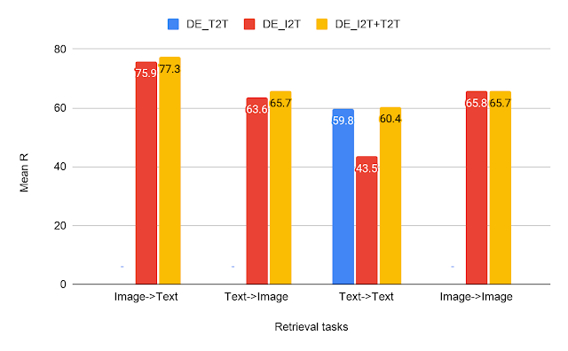
We ran a series of experiments to show the utility of CxC’s ratings. For this, we constructed three dual encoder (DE) models using BERT-base as the text encoder and EfficientNet-B4 as the image encoder:

  1. A text-text (DE_T2T) model that uses a shared text encoder for both sides.
  2. An image-text model (DE_I2T) that uses the aforementioned text and image encoders, and includes a layer above the text encoder to match the image encoder output.
  3. A multitask model (DE_I2T+T2T) trained on a weighted combination of text-text and image-text tasks.
CxC retrieval results — a comparison of our text-text (T2T), image-text (I2T) and multitask (I2T+T2T) dual encoder models on all the four retrieval tasks.

From the results on the retrieval tasks, we can see that DE_I2T+T2T (yellow bar) performs better than DE_I2T (red bar) on the image-text and text-image retrieval tasks. Thus, adding the intramodal (text-text) training task helped improve the intermodal (image-text, text-image) performance. As for the other two intramodal tasks (text-text and image-image), DE_I2T+T2T shows strong, balanced performance on both of them.

CxC correlation results for the same models shown above.

For the correlation tasks, DE_I2T performs the best on SIS and DE_I2T+T2T is the best overall. The correlation scores also show that DE_I2T performs well only on images: it has the highest SIS but has much worse STS. Adding the text-text loss to DE_I2T training (DE_I2T+T2T) produces more balanced overall performance.

The CxC dataset provides a much more complete set of relationships between and among images and captions than the raw MS-COCO image-caption pairs. The new ratings have been released and further details are in our paper. We hope to encourage the research community to push the state of the art on the tasks introduced by CxC with better models for jointly learning inter- and intra-modal representations.

Acknowledgments
The core team includes Daniel Cer, Yinfei Yang and Austin Waters. We thank Julia Hockenmaier for her inputs on CxC’s formulation, the Google Data Compute Team, especially Ashwin Kakarla and Mohd Majeed for their tooling and annotation support, Yuan Zhang, Eugene Ie for their comments on the initial versions of the paper and Daphne Luong for executive support for the data collection.


  *All the images in the article have been taken from the Open Images dataset under the CC-by 4.0 license. 

Source: Google AI Blog


RxR: A Multilingual Benchmark for Navigation Instruction Following

A core challenge in machine learning (ML) is to build agents that can navigate complex human environments in response to spoken or written commands. While today’s agents, including robots, can often navigate complicated environments, they cannot yet understand navigation goals expressed in natural language, such as, “Go past the brown double doors that are closed to your right and stand behind the chair at the head of the table.”

This challenge, referred to as vision-and-language navigation (VLN), demands a sophisticated understanding of spatial language. For example, the ability to identify the position “behind the chair at the head of the table requires finding the table, identifying which part of the table is considered to be the “head”, finding the chair closest to the head, identifying the area behind this chair and so on. While people can follow these instructions easily, these challenges cannot be easily solved with current ML-based methods, requiring systems that can better connect language to the physical world it describes.

To help spur progress in this area, we are excited to introduce Room-Across-Room (RxR), a new dataset for VLN. Described in “Room-Across-Room: Multilingual Vision-and-Language Navigation with Dense Spatiotemporal Grounding”, RxR is the first multilingual dataset for VLN, containing 126,069 human-annotated navigation instructions in three typologically diverse languages — English, Hindi and Telugu. Each instruction describes a path through a photorealistic simulator populated with indoor environments from the Matterport3D dataset, which includes 3D captures of homes, offices and public buildings. To track progress on VLN, we are also announcing the RxR Challenge, a competition that encourages the machine learning community to train and evaluate their own instruction following agents on RxR instructions.

Language Instruction
en-US Starting next to the long dining room table, turn so the table is to your right. Walk towards the glass double doors. When you reach the mat before the doors, turn immediately left and walk down the stairs. When you reach the bottom of the stairs, walk through the open doors to your left and continue through the art exhibit with the tub to your right hand side. Down the length of the table until you reach the small step at the end of the room before you reach the tub and stop.
  
hi-IN अभी हमारे बायीं ओर एक बड़ा मेज़ है कुछ कुर्सियाँ हैं और कुछ दीपक मेज़ के ऊपर रखे हैं। उलटी दिशा में घूम जाएँ और सिधा चलें। अभी हमारे दायीं ओर एक गोल मेज़ है वहां से सीधा बढ़ें और सामने एक शीशे का बंद दरवाज़ा है उससे पहले बायीं ओर एक सीढ़ी है उससे निचे उतरें। निचे उतरने के बाद दायीं ओर मुड़े और एक भूरे रंग के दरवाज़े से अंदर प्रवेश करें और सीधा चलें। अभी हमारे दायीं ओर एक बड़ा मेज़ है और दो कुर्सियां राखी हैं सीधा आगे बढ़ें। हमारे सामने एक पानी का कल है और सामने तीन कुर्सियां दिवार के पास रखी हैं यहीं पर ठहर जाएँ।
  
te-IN ఉన్న చోటు నుండి వెనకకు తిరిగి, నేరుగా వెళ్తే, మీ ముందర ఒక బల్ల ఉంటుంది. దాన్ని దాటుకొని ఎడమవైపుకి తిరిగితే, మీ ముందర మెట్లు ఉంటాయి. వాటిని పూర్తిగా దిగండి. ఇప్పుడు మీ ముందర రెండు తెరిచిన ద్వారాలు ఉంటాయి. ఎడమవైపు ఉన్న ద్వారం గుండా బయటకు వెళ్ళి, నేరుగా నడవండి. ఇప్పుడు మీ కుడివైపున పొడవైన బల్ల ఉంటుంది. దాన్ని దాటుకొని ముందరే ఉన్న మెట్ల వద్దకు వెళ్ళి ఆగండి.

Examples of English, Hindi and Telugu navigation instructions from the RxR dataset. Each navigation instruction describes the same path.

Pose Traces
In addition to navigation instructions and paths, RxR also includes a new, more detailed multimodal annotation called a pose trace. Inspired by the mouse traces captured in the Localized Narratives dataset, pose traces provide dense groundings between language, vision and movement in a rich 3D setting. To generate navigation instructions, we ask guide annotators to move along a path in the simulator while narrating the path based on the surroundings. The pose trace is a record of everything the guide sees along the path, time-aligned with the words in the navigation instructions. These traces are then paired with pose traces from follower annotators, who are tasked with following the intended path by listening to the guide’s audio, thereby validating the quality of the navigation instructions. Pose traces implicitly capture notions of landmark selection and visual saliency, and represent a play-by-play account of how to solve the navigation instruction generation task (for guides) and the navigation instruction following task (for followers).

Example English navigation instruction in the RxR dataset. Words in the instruction text (right) are color-coded to align with the pose trace (left) that illustrates the movements and visual percepts of the guide annotator as they move through the environment describing the path.
The same RxR example with words in the navigation instruction aligned to 360° images along the path. The parts of the scene the guide annotator observed are highlighted; parts of the scene ignored by the annotator are faded. Red and yellow boxes highlight some of the close alignments between the textual instructions and the annotator's visual cues. The red cross indicates the next direction the annotator moved.

Scale
In total, RxR contains almost 10 million words, making it around 10 times larger than existing datasets, such as R2R and Touchdown/Retouchdown. This is important because, in comparison to tasks based on static image and text data, language tasks that require learning through movement or interaction with an environment typically suffer from a lack of large-scale training data. RxR also addresses known biases in the construction of the paths that have arisen in other datasets, such as R2R in which all paths have similar lengths and take the shortest route to the goal. In contrast, the paths in RxR are on average longer and less predictable, making them more challenging to follow and encouraging models trained on the dataset to place greater emphasis on the role of language in the task. The size, scope and detail of RxR will expand the frontier for research on grounded language learning while reducing the dominance of high resource languages such as English.

Left: RxR is an order of magnitude larger than similar existing datasets. Right: Compared to R2R, the paths in RxR are typically longer and less predictable, making them more challenging to follow.

Baselines
To better characterize and understand the RxR dataset, we trained a variety of agents on RxR using our open source framework VALAN, and language representations from the multilingual BERT model. We found that results were improved by including follower annotations as well as guide annotations during training, and that independently trained monolingual agents outperformed a single multilingual agent.

Conceptually, evaluation of these agents is straightforward — did the agent follow the intended path? Empirically, we measure the similarity between the path taken by the VLN agent and the reference path using NDTW, a normalized measure of path fidelity that ranges between 100 (perfect correspondence) and 0 (completely wrong). The average score for the follower annotators across all three languages is 79.5, due to natural variation between similar paths. In contrast, the best model (a composite of three independently trained monolingual agents, one for each language) achieved an NDTW score on the RxR test set of 41.5. While this is much better than random (15.4), it remains far below human performance. Although advances in language modeling continue to rapidly erode the headroom for improvement in text-only language understanding benchmarks such as GLUE and SuperGLUE, benchmarks like RxR that connect language to the physical world offer substantial room for improvement.

Results for our multilingual and monolingual instruction following agents on the RxR test-standard split. While performance is much better than a random walk, there remains considerable headroom to reach human performance on this task.

Competition
To encourage further research in this area, we are launching the RxR Challenge, an ongoing competition for the machine learning community to develop computational agents that can follow natural language navigation instructions. To take part, participants upload the navigation paths taken by their agent in response to the provided RxR test instructions. In the most difficult setting (reported here and in the paper), all the test environments are previously unseen. However, we also allow for settings in which the agent is either trained in or explores the test environments in advance. For more details and the latest results please visit the challenge website.

PanGEA
We are also releasing the custom web-based annotation tool that we developed to collect the RxR dataset. The Panoramic Graph Environment Annotation toolkit (PanGEA), is a lightweight and customizable codebase for collecting speech and text annotations in panoramic graph environments, such as Matterport3D and StreetLearn. It includes speech recording and virtual pose tracking, as well as tooling to align the resulting pose trace with a manual transcript. For more details please visit the PanGEA github page.

Acknowledgements
The authors would like to thank Roma Patel, Eugene Ie and Jason Baldridge for their contributions to this research. We would also like to thank all the annotators, Sneha Kudugunta for analyzing the Telugu annotations, and Igor Karpov, Ashwin Kakarla and Christina Liu for their tooling and annotation support for this project, Austin Waters and Su Wang for help with image features, and Daphne Luong for executive support for the data collection.

Source: Google AI Blog


Enhancing the Research Community’s Access to Street View Panoramas for Language Grounding Tasks


Significant advances continue to be made in both natural language processing and computer vision, but the research community is still far from having computer agents that can interpret instructions in a real-world visual context and take appropriate actions based on those instructions. Agents, including robots, can learn to navigate new environments, but they cannot yet understand instructions such as, “Go forward and turn left after the red fire hydrant by the train tracks. Then go three blocks and stop in front of the building with a row of flags over its entrance.” Doing so requires relating verbal descriptions like train tracks, red fire hydrant, and row of flags to their visual appearance, understanding what a block is and how to count three of them, relating objects based on spatial configurations such as by and over, relating directions such as go forward and turn left to actions, and much more.

Grounded language understanding problems of this form are excellent testbeds for research on computational intelligence in that they are easy for people but hard for current agents, they synthesize language, perception and action, and evaluation of successful completion is straightforward. Progress on such problems can greatly enhance the ability of agents to coordinate movement and action with people. However finding or creating datasets large and diverse enough for developing robust models is difficult.

An ideal resource for quickly training and evaluating agents on grounded language understanding tasks is Street View imagery, an extensive and visually rich virtual representation of the world. Street View is integrated with Google Maps and is composed of billions of street-level panoramas. The Touchdown dataset, created by researchers at Cornell Tech, represents a compelling example of using Street View to drive research on grounded language understanding. However, due to restrictions on access to Street View panoramas, Touchdown can only provide panorama IDs rather than the panoramas themselves, sometimes making it difficult for the broader research community to work on Touchdown’s tasks: vision-and-language navigation (VLN), in which instructions are presented for navigation through streets, and spatial description resolution (SDR), which requires resolving spatial descriptions from a given viewpoint.

In “Retouchdown: Adding Touchdown to StreetLearn as a Shareable Resource for Language Grounding Tasks in Street View,” we address this problem by adding the Street View panoramas referenced in the Touchdown tasks to the existing StreetLearn dataset. Using this data, we generate a model that is fully compatible with the tasks defined in Touchdown. Additionally, we have provided open source TensorFlow implementations for the Touchdown tasks as part of the VALAN toolkit.

Grounded Language Understanding Tasks
Touchdown’s two grounded language understanding tasks can be used as benchmarks for navigation models. VLN involves following instructions from one street location to another, while SDR requires identifying a point in a Street View panorama given a description based on its surrounding visual context. The two tasks are shown being performed together in the animation below.
Example animation of a person following Touchdown instructions: “Orient yourself so that the umbrellas are to the right. Go straight and take a right at the first intersection. At the next intersection there should be an old-fashioned store to the left. There is also a dinosaur mural to the right. Touchdown is on the back of the dinosaur.”
Touchdown’s VLN task is similar to that defined in the popular Room-to-Room dataset, except that Street View has far greater visual diversity and more degrees of freedom for movement. Performance of the baseline models in Touchdown leaves considerable headroom for innovation and improvement on many facets of the task, including linguistic and visual representations, their integration, and learning to take actions conditioned on them.

That said, while enabling the broader research community to work with Touchdown’s tasks, certain safeguards are needed to make it compliant with the Google Maps/Google Earth Terms of Service and protect the needs of both Google and individuals. For example, panoramas may not be mass downloaded, nor can they be stored indefinitely (for example, individuals may ask to remove specific panoramas). Therefore, researchers must periodically delete and refresh panoramas in order to work with the data while remaining compliant with these terms.

StreetLearn: A Dataset of Approved Panoramas for Research Use
An alternative way to interact with Street View panoramas was forged by DeepMind with the StreetLearn data release last year. With StreetLearn, interested researchers can fill out a form requesting access to a set of 114k panoramas for regions of New York City and Pittsburgh. Recently, StreetLearn has been used to support the StreetNav task suite, which includes training and evaluating agents that follow Google Maps directions. This is a VLN task like Touchdown and Room-to-Room; however, it differs greatly in that it does not use natural language provided by people.

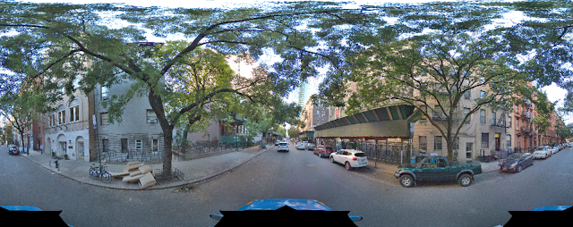
Additionally, even though StreetLearn’s panoramas cover the same area of Manhattan as Touchdown, they are not adequate for research covering the tasks defined in Touchdown, because those tasks require the exact panoramas that were used during the Touchdown annotation process. For example, in Touchdown tasks, the language instructions refer to transient objects such as cars, bicycles, and couches. A Street View panorama from a different time period may not contain these objects, so the instructions are not stable across time periods.
Touchdown instruction: “Two parked bicycles, and a discarded couch, all on the left. Walk just past this couch, and stop before you pass another parked bicycle. This bike will be white and red, with a white seat. Touchdown is sitting on top of the bike seat.” Other panoramas from the same location taken at other times would be highly unlikely to contain these exact items in the exact same positions. For a concrete example, see the current imagery available for this location in Street View, which contains very different transient objects.
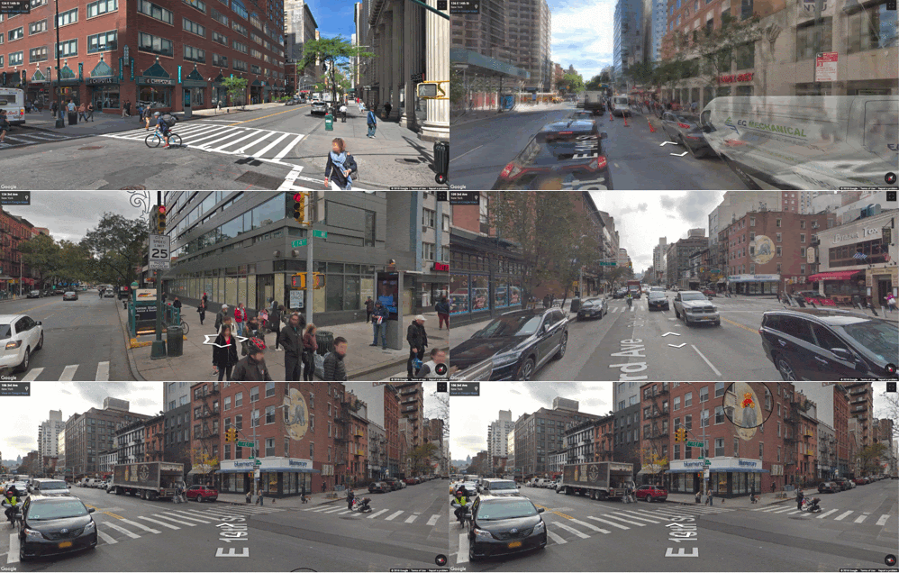
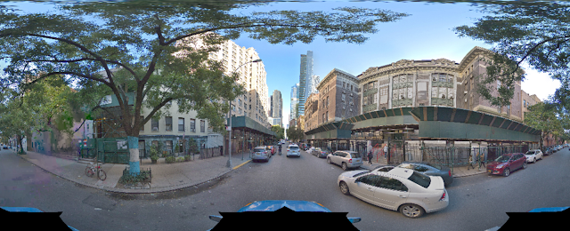
Furthermore, SDR requires coverage of multiple points-of-view for those specific panoramas. For example, the following panorama is one step down the street from the previous one. They may look similar, but they are in fact quite different — note that the bikes seen on the left side in both panoramas are not  the same — and the location of Touchdown is toward the middle of the above panorama (on the bike seat) and to the bottom left in the second panorama. As such, the pixel location of the SDR problem is different for different panoramas, but consistent with respect to the real world location referred to in the instruction. This is especially important for the end-to-end task of following both the VLN and SDR instructions together: if an agent stops, they should be able to complete the SDR task regardless of their exact location (provided the target is visible).
A panorama one step farther down the street from the previous scene.
Another problem is that the granularity of the panorama spacing is different. The figure below shows the overlap between the StreetLearn (blue) and Touchdown (red) panoramas in Manhattan. There are 710 panoramas (out of 29,641) that share the same ID in both datasets (in black). Touchdown covers half of Manhattan and the density of the panoramas is similar, but the exact locations of the nodes visited differ.
Adding Touchdown Panoramas to StreetLearn and Verifying Model Baselines
Retouchdown reconciles Touchdown’s mode of dissemination with StreetLearn’s, which was originally designed to adhere to the rights of Google and individuals while also simplifying access to researchers and improving reproducibility. Retouchdown includes both data and code that allows the broader research community to work effectively with the Touchdown tasks — most importantly to ensure access to the data and to ease reproducibility. To this end, we have integrated the Touchdown panoramas into the StreetLearn dataset to create a new version of StreetLearn with 144k panoramas (an increase of 26%) that are all approved for research use.

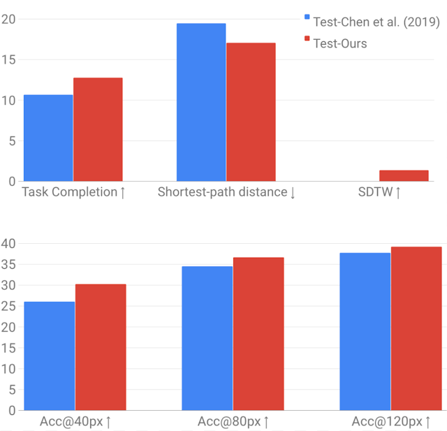
We also reimplemented models for VLN and SDR and show that they are on par or better than the results obtained in the original Touchdown paper. These implementations are open-sourced as well, as part of the VALAN toolkit. The first graph below compares the results of Chen et al. (2019) to our reimplementation for the VLN task. It includes the SDTW metric, which measures both successful completion and fidelity to the true reference path. The second graph below makes the same comparison for the SDR task. For SDR, we show accuracy@npx measurements, which provides the percent of times the model’s prediction is within n pixels of the goal location in the image. Our results are slightly better due to some small differences in models and processing, but most importantly, the results show that the updated panoramas are fully capable of supporting future modeling for the Touchdown tasks.
Performance comparison between Chen et al. (2019) using the original panoramas (in blue) and our reimplementation using the panoramas available in StreetLearn (in red). Top: VLN results for task completion, shortest path distance and success weighted by Dynamic Time Warping (SDTW). Bottom: SDR results for the accuracy@npx metrics.
Obtaining the Data
Researchers interested in working with the panoramas should fill out the StreetLearn interest form. Subject to approval, they will be provided with a download link. Their information is held so that the StreetLearn team can inform them of updates to the data. This allows both Google and participating researchers to effectively and easily respect takedown requests. The instructions and panorama connectivity data can be obtained from the Touchdown github repository.

It is our hope that this release of these additional panoramas will enable the research community to make further progress on these challenging grounded language understanding tasks.

Acknowledgements
The core team includes Yoav Artzi, Eugene Ie, and Piotr Mirowski. We would like to thank Howard Chen for his help with reproducing the Touchdown results, Larry Lansing, Valts Blukis and Vihan Jain for their help with the code and open-sourcing, and the Language team in Google Research, especially Radu Soricut, for the insightful comments that contributed to this work. Many thanks also to the Google Maps and Google Street View teams for their support in accessing and releasing the data, and to the Data Compute team for reviewing the panoramas.

Source: Google AI Blog


Graph-powered Machine Learning at Google


Recently, there have been significant advances in Machine Learning that enable computer systems to solve complex real-world problems. One of those advances is Google’s large scale, graph-based machine learning platform, built by the Expander team in Google Research. A technology that is behind many of the Google products and features you may use everyday, graph-based machine learning is a powerful tool that can be used to power useful features such as reminders in Inbox and smart messaging in Allo, or used in conjunction with deep neural networks to power the latest image recognition system in Google Photos.
Learning with Minimal Supervision

Much of the recent success in deep learning and machine learning, in general, can be attributed to models that demonstrate high predictive capacity when trained on large amounts of labeled data -- often millions of training examples. This is commonly referred to as “supervised learning” since it requires supervision, in the form of labeled data, to train the machine learning systems. (Conversely, some machine learning methods operate directly on raw data without any supervision, a paradigm referred to as unsupervised learning.)

However, the more difficult the task, the harder it is to get sufficient high-quality labeled data. It is often prohibitively labor intensive and time-consuming to collect labeled data for every new problem. This motivated the Expander research team to build new technology for powering machine learning applications at scale and with minimal supervision.

Expander’s technology draws inspiration from how humans learn to generalize and bridge the gap between what they already know (labeled information) and novel, unfamiliar observations (unlabeled information). Known as “semi-supervised” learning, this powerful technique enables us to build systems that can work in situations where training data may be sparse. One of the key advantages to a graph-based semi-supervised machine learning approach is the fact that (a) one models labeled and unlabeled data jointly during learning, leveraging the underlying structure in the data, (b) one can easily combine multiple types of signals (for example, relational information from Knowledge Graph along with raw features) into a single graph representation and learn over them. This is in contrast to other machine learning approaches, such as neural network methods, in which it is typical to first train a system using labeled data with features and then apply the trained system to unlabeled data.

Graph Learning: How It Works

At its core, Expander’s platform combines semi-supervised machine learning with large-scale graph-based learning by building a multi-graph representation of the data with nodes corresponding to objects or concepts and edges connecting concepts that share similarities. The graph typically contains both labeled data (nodes associated with a known output category or label) and unlabeled data (nodes for which no labels were provided). Expander’s framework then performs semi-supervised learning to label all nodes jointly by propagating label information across the graph.

However, this is easier said than done! We have to (1) learn efficiently at scale with minimal supervision (i.e., tiny amount of labeled data), (2) operate over multi-modal data (i.e., heterogeneous representations and various sources of data), and (3) solve challenging prediction tasks (i.e., large, complex output spaces) involving high dimensional data that might be noisy.

One of the primary ingredients in the entire learning process is the graph and choice of connections. Graphs come in all sizes, shapes and can be combined from multiple sources. We have observed that it is often beneficial to learn over multi-graphs that combine information from multiple types of data representations (e.g., image pixels, object categories and chat response messages for PhotoReply in Allo). The Expander team’s graph learning platform automatically generates graphs directly from data based on the inferred or known relationships between data elements. The data can be structured (for example, relational data) or unstructured (for example, sparse or dense feature representations extracted from raw data).

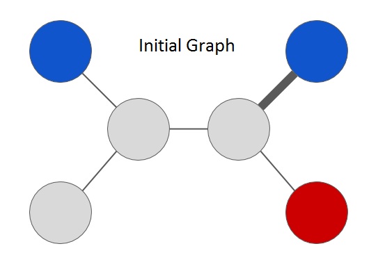
To understand how Expander’s system learns, let us consider an example graph shown below.
There are two types of nodes in the graph: “grey” represents unlabeled data whereas the colored nodes represent labeled data. Relationships between node data is represented via edges and thickness of each edge indicates strength of the connection. We can formulate the semi-supervised learning problem on this toy graph as follows: predict a color (“red” or “blue”) for every node in the graph. Note that the specific choice of graph structure and colors depend on the task. For example, as shown in this research paper we recently published, a graph that we built for the Smart Reply feature in Inbox represents email messages as nodes and colors indicate semantic categories of user responses (e.g., “yes”, “awesome”, “funny”).

The Expander graph learning framework solves this labeling task by treating it as an optimization problem. At the simplest level, it learns a color label assignment for every node in the graph such that neighboring nodes are assigned similar colors depending on the strength of their connection. A naive way to solve this would be to try to learn a label assignment for all nodes at once -- this method does not scale to large graphs. Instead, we can optimize the problem formulation by propagating colors from labeled nodes to their neighbors, and then repeating the process. In each step, an unlabeled node is assigned a label by inspecting color assignments of its neighbors. We can update every node’s label in this manner and iterate until the whole graph is colored. This process is a far more efficient way to optimize the same problem and the sequence of iterations converges to a unique solution in this case. The solution at the end of the graph propagation looks something like this:
Semi-supervised learning on a graph
In practice, we use complex optimization functions defined over the graph structure, which incorporate additional information and constraints for semi-supervised graph learning that can lead to hard, non-convex problems. The real challenge, however, is to scale this efficiently to graphs containing billions of nodes, trillions of edges and for complex tasks involving billions of different label types.

To tackle this challenge, we created an approach outlined in Large Scale Distributed Semi-Supervised Learning Using Streaming Approximation, published last year. It introduces a streaming algorithm to process information propagated from neighboring nodes in a distributed manner that makes it work on very large graphs. In addition, it addresses other practical concerns, notably it guarantees that the space complexity or memory requirements of the system stays constant regardless of the difficulty of the task, i.e., the overall system uses the same amount of memory regardless of whether the number of prediction labels is two (as in the above toy example) or a million or even a billion. This enables wide-ranging applications for natural language understanding, machine perception, user modeling and even joint multimodal learning for tasks involving multiple modalities such as text, image and video inputs.

Language Graphs for Learning Humor

As an example use of graph-based machine learning, consider emotion labeling, a language understanding task in Smart Reply for Inbox, where the goal is to label words occurring in natural language text with their fine-grained emotion categories. A neural network model is first applied to a text corpus to learn word embeddings, i.e., a mathematical vector representation of the meaning of each word. The dense embedding vectors are then used to build a sparse graph where nodes correspond to words and edges represent semantic relationship between them. Edge strength is computed using similarity between embedding vectors — low similarity edges are ignored. We seed the graph with emotion labels known a priori for a few nodes (e.g., laugh is labeled as “funny”) and then apply semi-supervised learning over the graph to discover emotion categories for remaining words (e.g., ROTFL gets labeled as “funny” owing to its multi-hop semantic connection to the word “laugh”).
Learning emotion associations using graph constructed from word embedding vectors
For applications involving large datasets or dense representations that are observed (e.g., pixels from images) or learned using neural networks (e.g., embedding vectors), it is infeasible to compute pairwise similarity between all objects to construct edges in the graph. The Expander team solves this problem by leveraging approximate, linear-time graph construction algorithms.

Graph-based Machine Intelligence in Action

The Expander team’s machine learning system is now being used on massive graphs (containing billions of nodes and trillions of edges) to recognize and understand concepts in natural language, images, videos, and queries, powering Google products for applications like reminders, question answering, language translation, visual object recognition, dialogue understanding, and more.

We are excited that with the recent release of Allo, millions of chat users are now experiencing smart messaging technology powered by the Expander team’s system for understanding and assisting with chat conversations in multiple languages. Also, this technology isn’t used only for large-scale models in the cloud - as announced this past week, Android Wear has opened up an on-device Smart Reply capability for developers that will provide smart replies for any messaging application. We’re excited to tackle even more challenging Internet-scale problems with Expander in the years to come.

Acknowledgements

We wish to acknowledge the hard work of all the researchers, engineers, product managers, and leaders across Google who helped make this technology a success. In particular, we would like to highlight the efforts of Allan Heydon, Andrei Broder, Andrew Tomkins, Ariel Fuxman, Bo Pang, Dana Movshovitz-Attias, Fritz Obermeyer, Krishnamurthy Viswanathan, Patrick McGregor, Peter Young, Robin Dua, Sujith Ravi and Vivek Ramavajjala.