Tag Archives: Machine Perception

Supercharge your Computer Vision models with the TensorFlow Object Detection API

Crossposted on the Google Research Blog

At Google, we develop flexible state-of-the-art machine learning (ML) systems for computer vision that not only can be used to improve our products and services, but also spur progress in the research community. Creating accurate ML models capable of localizing and identifying multiple objects in a single image remains a core challenge in the field, and we invest a significant amount of time training and experimenting with these systems.
Detected objects in a sample image (from the COCO dataset) made by one of our models.
Image credit: Michael Miley, original image
Last October, our in-house object detection system achieved new state-of-the-art results, and placed first in the COCO detection challenge. Since then, this system has generated results for a number of research publications1,2,3,4,5,6,7 and has been put to work in Google products such as NestCam, the similar items and style ideas feature in Image Search and street number and name detection in Street View.

Today we are happy to make this system available to the broader research community via the TensorFlow Object Detection API. This codebase is an open source framework built on top of TensorFlow that makes it easy to construct, train and deploy object detection models.  Our goals in designing this system was to support state-of-the-art models while allowing for rapid exploration and research.  Our first release contains the following:
The SSD models that use MobileNet are lightweight, so that they can be comfortably run in real time on mobile devices. Our winning COCO submission in 2016 used an ensemble of the Faster RCNN models, which are are more computationally intensive but significantly more accurate.  For more details on the performance of these models, see our CVPR 2017 paper.

Are you ready to get started?
We’ve certainly found this code to be useful for our computer vision needs, and we hope that you will as well.  Contributions to the codebase are welcome and please stay tuned for our own further updates to the framework. To get started, download the code here and try detecting objects in some of your own images using the Jupyter notebook, or training your own pet detector on Cloud ML engine!

By Jonathan Huang, Research Scientist and Vivek Rathod, Software Engineer

Acknowledgements
The release of the Tensorflow Object Detection API and the pre-trained model zoo has been the result of widespread collaboration among Google researchers with feedback and testing from product groups. In particular we want to highlight the contributions of the following individuals:

Core Contributors: Derek Chow, Chen Sun, Menglong Zhu, Matthew Tang, Anoop Korattikara, Alireza Fathi, Ian Fischer, Zbigniew Wojna, Yang Song, Sergio Guadarrama, Jasper Uijlings, Viacheslav Kovalevskyi, Kevin Murphy

Also special thanks to: Andrew Howard, Rahul Sukthankar, Vittorio Ferrari, Tom Duerig, Chuck Rosenberg, Hartwig Adam, Jing Jing Long, Victor Gomes, George Papandreou, Tyler Zhu

References
  1. Speed/accuracy trade-offs for modern convolutional object detectors, Huang et al., CVPR 2017 (paper describing this framework)
  2. Towards Accurate Multi-person Pose Estimation in the Wild, Papandreou et al., CVPR 2017
  3. YouTube-BoundingBoxes: A Large High-Precision Human-Annotated Data Set for Object Detection in Video, Real et al., CVPR 2017 (see also our blog post)
  4. Beyond Skip Connections: Top-Down Modulation for Object Detection, Shrivastava et al., arXiv preprint arXiv:1612.06851, 2016
  5. Spatially Adaptive Computation Time for Residual Networks, Figurnov et al., CVPR 2017
  6. AVA: A Video Dataset of Spatio-temporally Localized Atomic Visual Actions, Gu et al., arXiv preprint arXiv:1705.08421, 2017
  7. MobileNets: Efficient convolutional neural networks for mobile vision applications, Howard et al., arXiv preprint arXiv:1704.04861, 2017
MobileNets: Open Source Models for Efficient On-Device Vision

Crossposted on the Google Research Blog

Deep learning has fueled tremendous progress in the field of computer vision in recent years, with neural networks repeatedly pushing the frontier of visual recognition technology. While many of those technologies such as object, landmark, logo and text recognition are provided for internet-connected devices through the Cloud Vision API, we believe that the ever-increasing computational power of mobile devices can enable the delivery of these technologies into the hands of our users, anytime, anywhere, regardless of internet connection. However, visual recognition for on device and embedded applications poses many challenges — models must run quickly with high accuracy in a resource-constrained environment making use of limited computation, power and space.

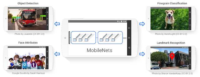
Today we are pleased to announce the release of MobileNets, a family of mobile-first computer vision models for TensorFlow, designed to effectively maximize accuracy while being mindful of the restricted resources for an on-device or embedded application. MobileNets are small, low-latency, low-power models parameterized to meet the resource constraints of a variety of use cases. They can be built upon for classification, detection, embeddings and segmentation similar to how other popular large scale models, such as Inception, are used.
Example use cases include detection, fine-grain classification, attributes and geo-localization.
This release contains the model definition for MobileNets in TensorFlow using TF-Slim, as well as 16 pre-trained ImageNet classification checkpoints for use in mobile projects of all sizes. The models can be run efficiently on mobile devices with TensorFlow Mobile.
Model Checkpoint
Million MACs
Million Parameters
Top-1 Accuracy
Top-5 Accuracy
569
4.24
70.7
89.5
418
4.24
69.3
88.9
291
4.24
67.2
87.5
186
4.24
64.1
85.3
317
2.59
68.4
88.2
233
2.59
67.4
87.3
162
2.59
65.2
86.1
104
2.59
61.8
83.6
150
1.34
64.0
85.4
110
1.34
62.1
84.0
77
1.34
59.9
82.5
49
1.34
56.2
79.6
41
0.47
50.6
75.0
34
0.47
49.0
73.6
21
0.47
46.0
70.7
14
0.47
41.3
66.2
Choose the right MobileNet model to fit your latency and size budget. The size of the network in memory and on disk is proportional to the number of parameters. The latency and power usage of the network scales with the number of Multiply-Accumulates (MACs) which measures the number of fused Multiplication and Addition operations. Top-1 and Top-5 accuracies are measured on the ILSVRC dataset.
We are excited to share MobileNets with the open source community. Information for getting started can be found at the TensorFlow-Slim Image Classification Library. To learn how to run models on-device please go to TensorFlow Mobile. You can read more about the technical details of MobileNets in our paper, MobileNets: Efficient Convolutional Neural Networks for Mobile Vision Applications.

By Andrew G. Howard, Senior Software Engineer and Menglong Zhu, Software Engineer

Acknowledgements
MobileNets were made possible with the hard work of many engineers and researchers throughout Google. Specifically we would like to thank:

Core Contributors: Andrew G. Howard, Menglong Zhu, Bo Chen, Dmitry Kalenichenko, Weijun Wang, Tobias Weyand, Marco Andreetto, Hartwig Adam

Special thanks to: Benoit Jacob, Skirmantas Kligys, George Papandreou, Liang-Chieh Chen, Derek Chow, Sergio Guadarrama, Jonathan Huang, Andre Hentz, Pete Warden

MobileNets: Open-Source Models for Efficient On-Device Vision


Deep learning has fueled tremendous progress in the field of computer vision in recent years, with neural networks repeatedly pushing the frontier of visual recognition technology. While many of those technologies such as object, landmark, logo and text recognition are provided for internet-connected devices through the Cloud Vision API, we believe that the ever-increasing computational power of mobile devices can enable the delivery of these technologies into the hands of our users, anytime, anywhere, regardless of internet connection. However, visual recognition for on device and embedded applications poses many challenges — models must run quickly with high accuracy in a resource-constrained environment making use of limited computation, power and space.

Today we are pleased to announce the release of MobileNets, a family of mobile-first computer vision models for TensorFlow, designed to effectively maximize accuracy while being mindful of the restricted resources for an on-device or embedded application. MobileNets are small, low-latency, low-power models parameterized to meet the resource constraints of a variety of use cases. They can be built upon for classification, detection, embeddings and segmentation similar to how other popular large scale models, such as Inception, are used.
Example use cases include detection, fine-grain classification, attributes and geo-localization.
This release contains the model definition for MobileNets in TensorFlow using TF-Slim, as well as 16 pre-trained ImageNet classification checkpoints for use in mobile projects of all sizes. The models can be run efficiently on mobile devices with TensorFlow Mobile.

Model Checkpoint
Million MACs
Million Parameters
Top-1 Accuracy
Top-5 Accuracy
569
4.24
70.7
89.5
418
4.24
69.3
88.9
291
4.24
67.2
87.5
186
4.24
64.1
85.3
317
2.59
68.4
88.2
233
2.59
67.4
87.3
162
2.59
65.2
86.1
104
2.59
61.8
83.6
150
1.34
64.0
85.4
110
1.34
62.1
84.0
77
1.34
59.9
82.5
49
1.34
56.2
79.6
41
0.47
50.6
75.0
34
0.47
49.0
73.6
21
0.47
46.0
70.7
14
0.47
41.3
66.2
Choose the right MobileNet model to fit your latency and size budget. The size of the network in memory and on disk is proportional to the number of parameters. The latency and power usage of the network scales with the number of Multiply-Accumulates (MACs) which measures the number of fused Multiplication and Addition operations. Top-1 and Top-5 accuracies are measured on the ILSVRC dataset.
We are excited to share MobileNets with the open-source community. Information for getting started can be found at the TensorFlow-Slim Image Classification Library. To learn how to run models on-device please go to TensorFlow Mobile. You can read more about the technical details of MobileNets in our paper, MobileNets: Efficient Convolutional Neural Networks for Mobile Vision Applications.

Acknowledgements
MobileNets were made possible with the hard work of many engineers and researchers throughout Google. Specifically we would like to thank:

Core Contributors: Andrew G. Howard, Menglong Zhu, Bo Chen, Dmitry Kalenichenko, Weijun Wang, Tobias Weyand, Marco Andreetto, Hartwig Adam

Special thanks to: Benoit Jacob, Skirmantas Kligys, George Papandreou, Liang-Chieh Chen, Derek Chow, Sergio Guadarrama, Jonathan Huang, Andre Hentz, Pete Warden

Announcing AudioSet: A Dataset for Audio Event Research


Systems able to recognize sounds familiar to human listeners have a wide range of applications, from adding sound effect information to automatic video captions, to potentially allowing you to search videos for specific audio events. Building Deep Learning systems to do this relies heavily on both a large quantity of computing (often from highly parallel GPUs), and also – and perhaps more importantly – on significant amounts of accurately-labeled training data. However, research in environmental sound recognition is limited by currently available public datasets.

In order to address this, we recently released AudioSet, a collection of over 2 million ten-second YouTube excerpts labeled with a vocabulary of 527 sound event categories, with at least 100 examples for each category. Announced in our paper at the IEEE International Conference on Acoustics, Speech, and Signal Processing, AudioSet provides a common, realistic-scale evaluation task for audio event detection and a starting point for a comprehensive vocabulary of sound events, designed to advance research into audio event detection and recognition.
Developing an Ontology
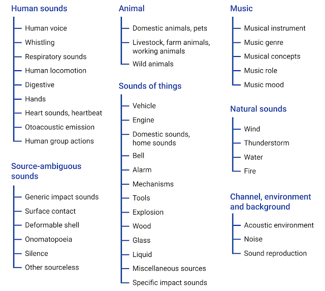
When we started on this work last year, our first task was to define a vocabulary of sound classes that provided a consistent level of detail over the spectrum of sound events we planned to label. Defining this ontology was necessary to avoid problems of ambiguity and synonyms; without this, we might end up trying to differentiate “Timpani” from “Kettle drum”, or “Water tap” from “Faucet”. Although a number of scientists have looked at how humans organize sound events, the few existing ontologies proposed have been small and partial. To build our own, we searched the web for phrases like “Sounds, such as X and Y”, or “X, Y, and other sounds”. This gave us a list of sound-related words which we manually sorted into a hierarchy of over 600 sound event classes ranging from “Child speech” to “Ukulele” to “Boing”. To make our taxonomy as comprehensive as possible, we then looked at comparable lists of sound events (for instance, the Urban Sound Taxonomy) to add significant classes we may have missed and to merge classes that weren't well defined or well distinguished. You can explore our ontology here.
The top two levels of the AudioSet ontology.
From Ontology to Labeled Data
With our new ontology in hand, we were able to begin collecting human judgments of where the sound events occur. This, too, raises subtle problems: unlike the billions of well-composed photographs available online, people don’t typically produce “well-framed” sound recordings, much less provide them with captions. We decided to use 10 second sound snippets as our unit; anything shorter becomes very difficult to identify in isolation. We collected candidate snippets for each of our classes by taking random excerpts from YouTube videos whose metadata indicated they might contain the sound in question (“Dogs Barking for 10 Hours”). Each snippet was presented to a human labeler with a small set of category names to be confirmed (“Do you hear a Bark?”). Subsequently, we proposed snippets whose content was similar to examples that had already been manually verified to contain the class, thereby finding examples that were not discoverable from the metadata. Because some classes were much harder to find than others – particularly the onomatopoeia words like “Squish” and “Clink” – we adapted our segment proposal process to increase the sampling for those categories. For more details, see our paper on the matching technique.

AudioSet provides the URLs of each video excerpt along with the sound classes that the raters confirmed as present, as well as precalculated audio features from the same classifier used to generate audio features for the updated YouTube 8M Dataset. Below is a histogram of the number of examples per class:
The total number of videos for selected classes in AudioSet.
You can browse this data at the AudioSet website which lets you view all the 2 million excerpts for all the classes.
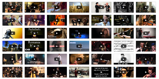
A few of the segments representing the class “Violin, fiddle”.
Quality Assessment
Once we had a substantial set of human ratings, we conducted an internal Quality Assessment task where, for most of the classes, we checked 10 examples of excerpts that the annotators had labeled with that class. This revealed a significant number of classes with inaccurate labeling: some, like “Dribble” (uneven water flow) and “Roll” (a hard object moving by rotating) had been systematically confused (as basketball dribbling and drum rolls, respectively); some such as “Patter” (footsteps of small animals) and “Sidetone” (background sound on a telephony channel) were too difficult to label and/or find examples for, even with our content-based matching. We also looked at the behavior of a classifier trained on the entire dataset and found a number of frequent confusions indicating separate classes that were not really distinct, such as “Jingle” and “Tinkle”.

To address these “problem” classes, we developed a re-rating process by labeling groups of classes that span (and thus highlight) common confusions, and created instructions for the labeler to be used with these sounds. This re-rating has led to multiple improvements – merged classes, expanded coverage, better descriptions – that we were able to incorporate in this release. This iterative process of labeling and assessment has been particularly effective in shaking out weaknesses in the ontology.

A Community Dataset
By releasing AudioSet, we hope to provide a common, realistic-scale evaluation task for audio event detection, as well as a starting point for a comprehensive vocabulary of sound events. We would like to see a vibrant sound event research community develop, including through external efforts such as the DCASE challenge series. We will continue to improve the size, coverage, and accuracy of this data and plan to make a second release in the coming months when our rerating process is complete. We additionally encourage the research community to continue to refine our ontology, which we have open sourced on GitHub. We believe that with this common focus, sound event recognition will continue to advance and will allow machines to understand sounds similar to the way we do, enabling new and exciting applications.

Acknowledgments:
AudioSet is the work of Jort F. Gemmeke, Dan Ellis, Dylan Freedman, Shawn Hershey, Aren Jansen, Wade Lawrence, Channing Moore, Manoj Plakal, and Marvin Ritter, with contributions from Sami Abu-El-Hajia, Sourish Chaudhuri, Victor Gomes, Nisarg Kothari, Dick Lyon, Sobhan Naderi Parizi, Paul Natsev, Brian Patton, Rif A. Saurous, Malcolm Slaney, Ron Weiss, and Kevin Wilson.

Headset “Removal” for Virtual and Mixed Reality


Virtual Reality (VR) enables remarkably immersive experiences, offering new ways to view the world and the ability to explore novel environments, both real and imaginary. However, compared to physical reality, sharing these experiences with others can be difficult, as VR headsets make it challenging to create a complete picture of the people participating in the experience.

Some of this disconnect is alleviated by Mixed Reality (MR), a related medium that shares the virtual context of a VR user in a two dimensional video format allowing other viewers to get a feel for the user’s virtual experience. Even though MR facilitates sharing, the headset continues to block facial expressions and eye gaze, presenting a significant hurdle to a fully engaging experience and complete view of the person in VR.

Google Machine Perception researchers, in collaboration with Daydream Labs and YouTube Spaces, have been working on solutions to address this problem wherein we reveal the user’s face by virtually “removing” the headset and create a realistic see-through effect.
VR user captured in front of a green-screen is blended with the virtual environment to generate the MR output: Traditional MR output has the user face occluded, while our result reveals the face. Note how the headset is modified with a marker to aid tracking.
Our approach uses a combination of 3D vision, machine learning and graphics techniques, and is best explained in the context of enhancing Mixed Reality video (also discussed in the Google-VR blog). It consists of three main components:

Dynamic face model capture
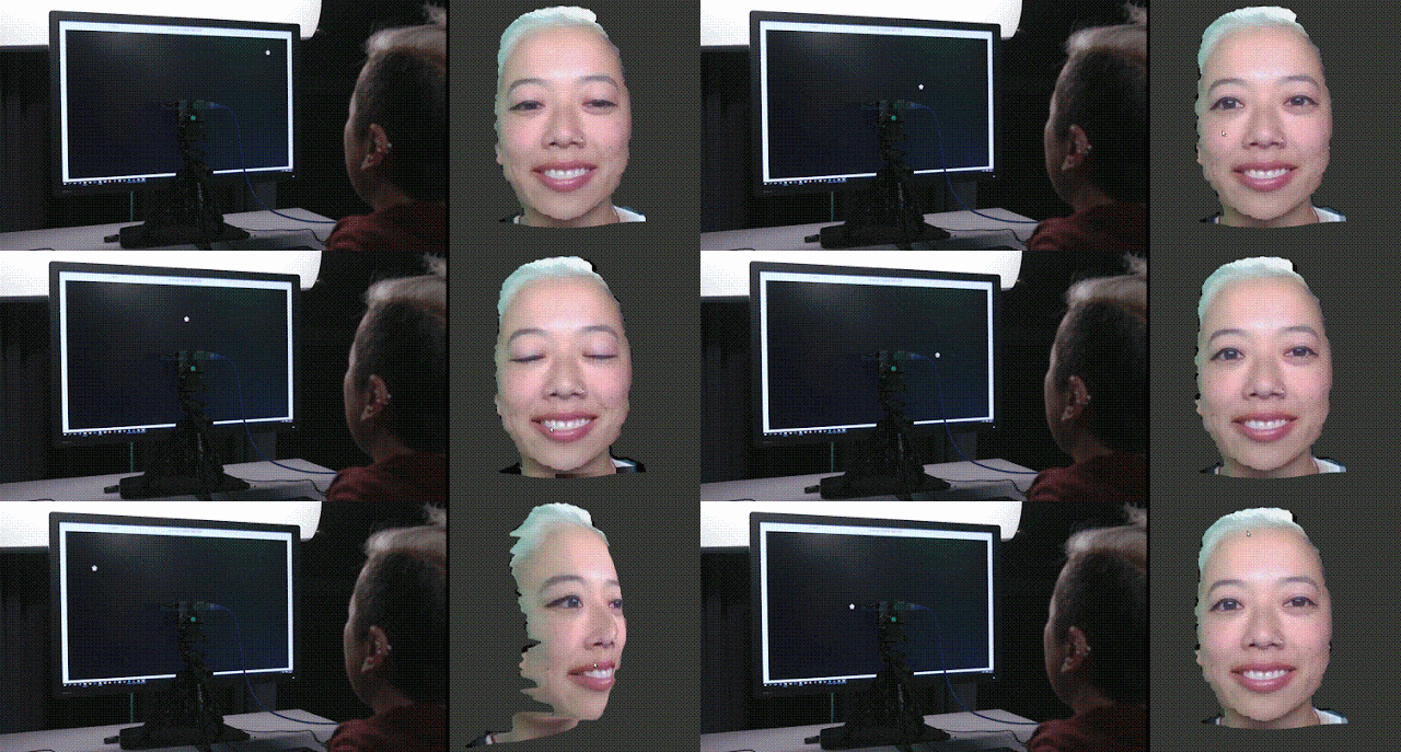
The core idea behind our technique is to use a 3D model of the user’s face as a proxy for the hidden face. This proxy is used to synthesize the face in the MR video, thereby creating an impression of the headset being removed. First, we capture a personalized 3D face model for the user with what we call gaze-dependent dynamic appearance. This initial calibration step requires the user to sit in front of a color+depth camera and a monitor, and then track a marker on the monitor with their eyes. We use this one-time calibration procedure — which typically takes less than a minute — to acquire a 3D face model of the user, and learn a database that maps appearance images (or textures) to different eye-gaze directions and blinks. This gaze database (i.e. the face model with textures indexed by eye-gaze) allows us to dynamically change the appearance of the face during synthesis and generate any desired eye-gaze, thus making the synthesized face look natural and alive
On the left, the user’s face is captured by a camera as she tracks a marker on the monitor with her eyes. On the right, we show the dynamic nature of reconstructed 3D face model: by moving or clicking on the mouse, we are able to simulate both apparent eye gaze and blinking.
Calibration and Alignment
Creating a Mixed Reality video requires a specialized setup consisting of an external camera, calibrated and time-synced with the headset. The camera captures a video stream of the VR user in front of a green screen and then composites a cutout of the user with the virtual world to create the final MR video. An important step here is to accurately estimate the calibration (the fixed 3D transformation) between the camera and headset coordinate systems. These calibration techniques typically involve significant manual intervention and are done in multiple steps. We simplify the process by adding a physical marker to the front of the headset and tracking it visually in 3D, which allows us to optimize for the calibration parameters automatically from the VR session.

For headset “removal”, we need to align the 3D face model with the visible portion of the face in the camera stream, so that they would blend seamlessly with each other. A reasonable proxy to this alignment is to place the face model just behind the headset. The calibration described above, coupled with VR headset tracking, provides sufficient information to determine this placement, allowing us to modify the camera stream by rendering the virtual face into it.

Compositing and Rendering
Having tackled the alignment, the last step involves producing a suitable rendering of the 3D face model, consistent with the content in the camera stream. We are able to reproduce the true eye-gaze of the user by combining our dynamic gaze database with an HTC Vive headset that has been modified by SMI to incorporate eye-tracking technology. Images from these eye trackers lack sufficient detail to directly reproduce the occluded face region, but are well suited to provide fine-grained gaze information. Using the live gaze data from the tracker, we synthesize a face proxy that accurately represents the user’s attention and blinks. At run-time, the gaze database, captured in the preprocessing step, is searched for the most appropriate face image corresponding to the query gaze state, while also respecting aesthetic considerations such as temporal smoothness. Additionally, to account for lighting changes between gaze database acquisition and run-time, we apply color correction and feathering, such that the synthesized face region matches with the rest of the face.

Humans are highly sensitive to artifacts on faces, and even small imperfections in synthesis of the occluded face can feel unnatural and distracting, a phenomenon known as the “uncanny valley.” To mitigate this problem, we do not remove the headset completely, instead we have chosen a user experience that conveys a ‘scuba mask effect’ by compositing the color corrected face proxy with a translucent headset. Reminding the viewer of the presence of the headset helps us avoid the uncanny valley, and also makes our algorithm robust to small errors in alignment and color correction.

This modified camera stream, displaying a see-through headset, with the user’s face revealed and their true eye-gaze recreated, is subsequently merged with the virtual environment to create the final MR video.

Results and Extensions
We have used our headset removal technology to enhance Mixed Reality, allowing the medium to not only convey a VR user’s interaction with the virtual environment but also show their face in a natural and convincing fashion. The example below demonstrates our tech applied to an artist using Google Tilt Brush in a virtual environment:
An artist creates 3D art using Google Tilt Brush, shown in Mixed Reality. On the top is the traditional MR result where the face is hidden behind the headset. On the bottom is our result, which reveals the entire face and eyes for a more natural and engaging experience.
While we have shown the potential of our technology, its applications extend beyond Mixed Reality. Headset removal is poised to enhance communication and social interaction in VR itself with diverse applications like VR video conference meetings, multiplayer VR gaming, and exploration with friends and family. Going from an utterly blank headset to being able to see, with photographic realism, the faces of fellow VR users promises to be a significant transition in the VR world, and we are excited to be a part of it.

An updated YouTube-8M, a video understanding challenge, and a CVPR workshop. Oh my!


Last September, we released the YouTube-8M dataset, which spans millions of videos labeled with thousands of classes, in order to spur innovation and advancement in large-scale video understanding. More recently, other teams at Google have released datasets such as Open Images and YouTube-BoundingBoxes that, along with YouTube-8M, can be used to accelerate image and video understanding. To further these goals, today we are releasing an update to the YouTube-8M dataset, and in collaboration with Google Cloud Machine Learning and kaggle.com, we are also organizing a video understanding competition and an affiliated CVPR’17 Workshop.

An Updated YouTube-8M
The new and improved YouTube-8M includes cleaner and more verbose labels (twice as many labels per video, on average), a cleaned-up set of videos, and for the first time, the dataset includes pre-computed audio features, based on a state-of-the-art audio modeling architecture, in addition to the previously released visual features. The audio and visual features are synchronized in time, at 1-second temporal granularity, which makes YouTube-8M a large-scale multi-modal dataset, and opens up opportunities for exciting new research on joint audio-visual (temporal) modeling. Key statistics on the new version are illustrated below (more details here).
A tree-map visualization of the updated YouTube-8M dataset, organized into 24 high-level verticals, including the top-200 most frequent entities, plus the top-5 entities for each vertical.
Sample videos from the top-18 high-level verticals in the YouTube-8M dataset.
The Google Cloud & YouTube-8M Video Understanding Challenge
We are also excited to announce the Google Cloud & YouTube-8M Video Understanding Challenge, in partnership with Google Cloud and kaggle.com. The challenge invites participants to build audio-visual content classification models using YouTube-8M as training data, and to then label ~700K unseen test videos. It will be hosted as a Kaggle competition, sponsored by Google Cloud, and will feature a $100,000 prize pool for the top performers (details here). In order to enable wider participation in the competition, Google Cloud is also offering credits so participants can optionally do model training and exploration using Google Cloud Machine Learning. Open-source TensorFlow code, implementing a few baseline classification models for YouTube-8M, along with training and evaluation scripts, is available at Github. For details on getting started with local or cloud-based training, please see our README and the getting started guide on Kaggle.

The CVPR 2017 Workshop on YouTube-8M Large-Scale Video Understanding
We will announce the results of the challenge and host invited talks by distinguished researchers at the 1st YouTube-8M Workshop, to be held July 26, 2017, at the 30th IEEE Conference on Computer Vision and Pattern Recognition (CVPR 2017) in Honolulu, Hawaii. The workshop will also feature presentations by top-performing challenge participants and a selected set of paper submissions. We invite researchers to submit papers describing novel research, experiments, or applications based on YouTube-8M dataset, including papers summarizing their participation in the above challenge.

We designed this dataset with scale and diversity in mind, and hope lessons learned here will generalize to many video domains (YouTube-8M captures over 20 diverse video domains). We believe the challenge can also accelerate research by enabling researchers without access to big data or compute clusters to explore and innovate at previously unprecedented scale. Please join us in advancing video understanding!

Acknowledgements
This post reflects the work of many others within Machine Perception at Google Research, including Sami Abu-El-Haija, Anja Hauth, Nisarg Kothari, Joonseok Lee, Hanhan Li, Sobhan Naderi Parizi, Rahul Sukthankar, George Toderici, Balakrishnan Varadarajan, Sudheendra Vijayanarasimhan, Jiang Wang, as well as Philippe Poutonnet and Mike Styer from Google Cloud, and our partners at Kaggle. We are grateful for the support and advice from many others at Google Research, Google Cloud, and YouTube, and especially thank Aren Jansen, Jort Gemmeke, Dan Ellis, and the Google Research Sound Understanding team for providing the audio features in the updated dataset.

Advancing Research on Video Understanding with the YouTube-BoundingBoxes Dataset


One of the most challenging research areas in machine learning today is enabling computers to understand what a scene is about. For example, while humans know that a ball that disappears behind a wall only to reappear a moment later is very likely the same object, this is not at all obvious to an algorithm. Understanding this requires not only a global picture of what objects are contained in each frame of a video, but also where those objects are located within the frame and their locations over time. Just last year we published YouTube-8M, a dataset consisting of automatically labelled YouTube videos. And while this helps further progress in the field, it is only one piece to the puzzle.

Today, in order to facilitate progress in video understanding research, we are introducing YouTube-BoundingBoxes, a dataset consisting of 5 million bounding boxes spanning 23 object categories, densely labeling segments from 210,000 YouTube videos. To date, this is the largest manually annotated video dataset containing bounding boxes, which track objects in temporally contiguous frames. The dataset is designed to be large enough to train large-scale models, and be representative of videos captured in natural settings. Importantly, the human-labelled annotations contain objects as they appear in the real world with partial occlusions, motion blur and natural lighting.
Summary of dataset statistics. Bar Chart: Relative number of detections in existing image (red) and video (blue) data sets. The YouTube BoundingBoxes dataset (YT-BB) is at the bottom, is at the bottom. Table: The three columns are counts for: classification annotations, bounding boxes, and unique videos with bounding boxes. Full details on the dataset can be found in the preprint.
A key feature of this dataset is that bounding box annotations are provided for entire video segments. These bounding box annotations may be used to train models that explicitly leverage this temporal information to identify, localize and track objects over time. In a video, individual annotated objects might become entirely occluded and later return in subsequent frames. These annotations of individual objects are sometimes not recognizable from individual frames, but can be understood and recognized in the context of the video if the objects are localized and tracked accurately.
Three video segments, sampled at 1 frame per second. The final frame of each example shows how it is visually challenging to recognize the bounded object, due to blur or occlusion (train example, blue arrow). However, temporally-related frames, where the object has been more clearly identified, can allow object classes to be inferred. Note how only visible parts are included in the box: the orange arrow in the bear example (middle row) points to the hidden head. The dog example illustrates tight bounding boxes that track the tail (orange arrows) and foot (blue arrows). The airplane example illustrates how partial objects are annotated (first frame) tracked across changes in perspective, occlusions and camera cuts.
We hope that this dataset might ultimately aid the computer vision and machine learning community and lead to new methods for analyzing and understanding real world vision problems. You can learn more about the dataset in this associated preprint.

Acknowledgements
The work was greatly helped along by Xin Pan and Thomas Silva, as well as support and advice from Manfred Georg, Sami Abu-El-Haija, Susanna Ricco and George Toderici.

Get moving with the new Motion Stills


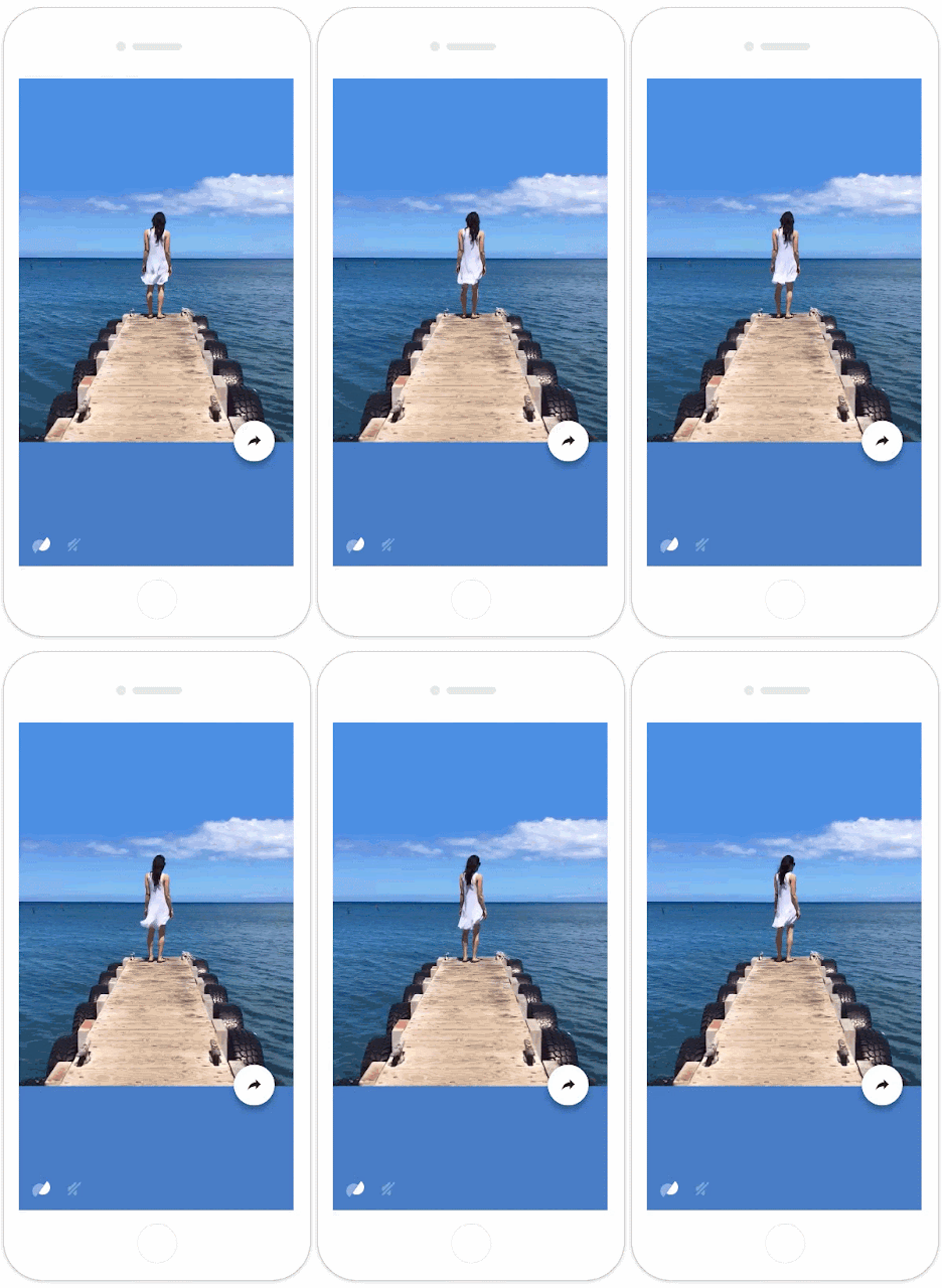
Last June, we released Motion Stills, an iOS app that uses our video stabilization technology to create easily shareable GIFs from Apple Live Photos. Since then, we integrated Motion Stills into Google Photos for iOS and thought of ways to improve it, taking into account your ideas for new features.

Today, we are happy to announce a major new update to the Motion Stills app that will help you create even more beautiful videos and fun GIFs using motion-tracked text overlays, super-resolution videos, and automatic cinemagraphs.

Motion Text

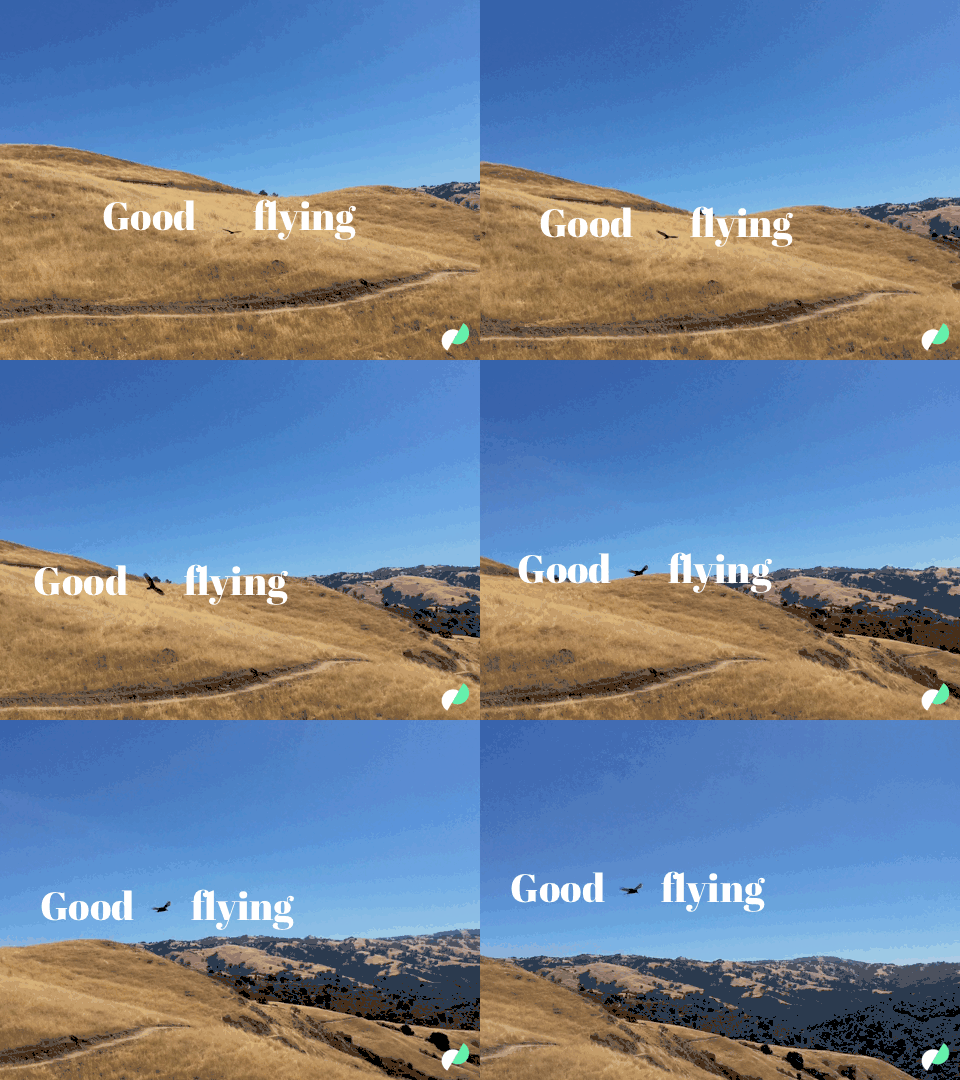
We’ve added motion text so you can create moving text effects, similar to what you might see in movies and TV shows, directly on your phone. With Motion Text, you can easily position text anywhere over your video to get the exact result you want. It only takes a second to initialize while you type, and a tracks at 1000 FPS throughout the whole Live Photo, so the process feels instantaneous.
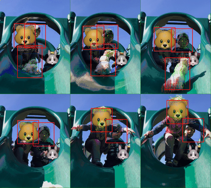
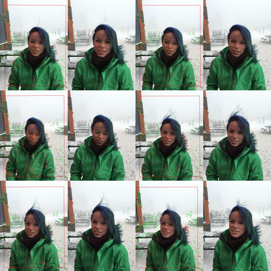
To make this possible, we took the motion tracking technology that we run on YouTube servers for “Privacy Blur”, and made it run even faster on your device. How? We first create motion metadata for your video by leveraging machine learning to classify foreground/background features as well as to model temporally coherent camera motion. We then take this metadata, and use it as input to an algorithm that can track individual objects while discriminating it from others. The algorithm models each object’s state that includes its motion in space, an implicit appearance model (described as a set of its moving parts), and its centroid and extent, as shown in the figure below.
Enhance! your videos with better detail and loops

Last month, we published the details of our state-of-the-art RAISR technology, which employs machine learning to create super-resolution detail in images. This technology is now available in Motion Stills, automatically sharpening every video you export.

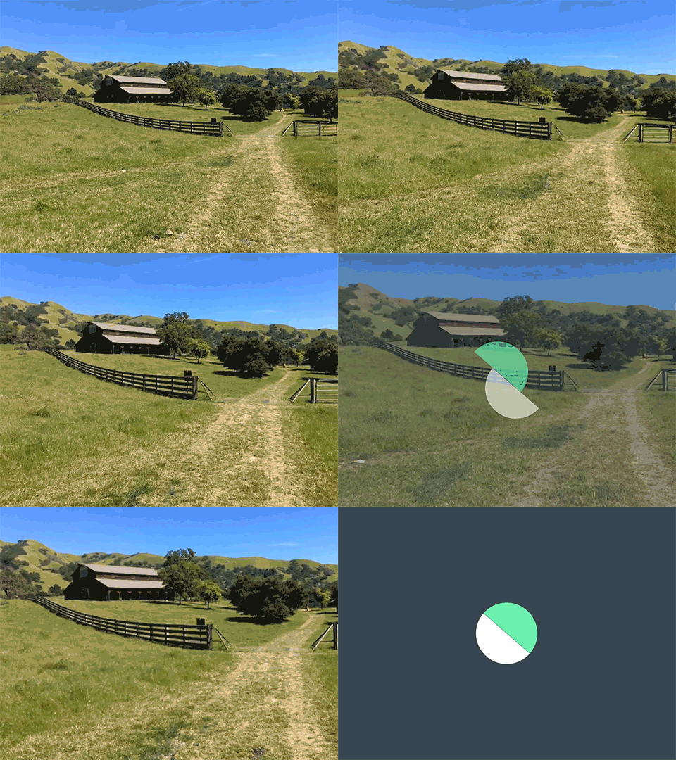
We are also going beyond stabilization to bring you fully automatic cinemagraphs. After freezing the background into a still photo, we analyze our result to optimize for the perfect loop transition. By considering a range of start and end frames, we build a matrix of transition scores between frame pairs. A significant minimum in this matrix reflects the perfect transition, resulting in an endless loop of motion stillness.
Continuing improve the experience

Thanks to your feedback, we’ve additionally rebuilt our navigation and added more tutorials. We’ve also added Apple’s 3D touch to let you “peek and pop” clips in your stream and movie tray. Lots more is coming to address your top requests, so please download the new release of Motion Stills and keep sending us feedback with #motionstills on your favorite social media.

Enhance! RAISR Sharp Images with Machine Learning


Everyday the web is used to share and store millions of pictures, enabling one to explore the world, research new topics of interest, or even share a vacation with friends and family. However, many of these images are either limited by the resolution of the device used to take the picture, or purposely degraded in order to accommodate the constraints of cell phones, tablets, or the networks to which they are connected. With the ubiquity of high-resolution displays for home and mobile devices, the demand for high-quality versions of low-resolution images, quickly viewable and shareable from a wide variety of devices, has never been greater.

With “RAISR: Rapid and Accurate Image Super-Resolution”, we introduce a technique that incorporates machine learning in order to produce high-quality versions of low-resolution images. RAISR produces results that are comparable to or better than the currently available super-resolution methods, and does so roughly 10 to 100 times faster, allowing it to be run on a typical mobile device in real-time. Furthermore, our technique is able to avoid recreating the aliasing artifacts that may exist in the lower resolution image.

Upsampling, the process of producing an image of larger size with significantly more pixels and higher image quality from a low quality image, has been around for quite a while. Well-known approaches to upsampling are linear methods which fill in new pixel values using simple, and fixed, combinations of the nearby existing pixel values. These methods are fast because they are fixed linear filters (a constant convolution kernel applied uniformly across the image). But what makes these upsampling methods fast, also makes them ineffective in bringing out vivid details in the higher resolution results. As you can see in the example below, the upsampled image looks blurry – one would hesitate to call it enhanced.
Left: Low-res original, Right: simple (bicubic) upsampled version (2x)

With RAISR, we instead use machine learning and train on pairs of images, one low quality, one high, to find filters that, when applied to selectively to each pixel of the low-res image, will recreate details that are of comparable quality to the original. RAISR can be trained in two ways. The first is the "direct" method, where filters are learned directly from low and high-resolution image pairs. The other method involves first applying a computationally cheap upsampler to the low resolution image (as in the figure above) and then learning the filters from the upsampled and high resolution image pairs. While the direct method is computationally faster, the 2nd method allows for non-integer scale factors and better leveraging of hardware-based upsampling.

For either method, RAISR filters are trained according to edge features found in small patches of images, - brightness/color gradients, flat/textured regions, etc. - characterized by direction (the angle of an edge), strength (sharp edges have a greater strength) and coherence (a measure of how directional the edge is). Below is a set of RAISR filters, learned from a database of 10,000 high and low resolution image pairs (where the low-res images were first upsampled). The training process takes about an hour.
Collection of learned 11x11 filters for 3x super-resolution. Filters can be learned for a range of super-resolution factors, including fractional ones. Note that as the angle of the edge changes, we see the angle of the filter rotate as well. Similarly, as the strength increases, the sharpness of the filters increases, and the anisotropy of the filter increases with rising coherence.

From left to right, we see that the learned filters correspond selectively to the direction of the underlying edge that is being reconstructed. For example, the filter in the middle of the bottom row is most appropriate for a strong horizontal edge (gradient angle of 90 degrees) with a high degree of coherence (a straight, rather than a curved, edge). If this same horizontal edge is low-contrast, then a different filter is selected such one in the top row.

In practice, at run-time RAISR selects and applies the most relevant filter from the list of learned filters to each pixel neighborhood in the low-resolution image. When these filters are applied to the lower quality image, they recreate details that are of comparable quality to the original high resolution, and offer a significant improvement to linear, bicubic, or Lanczos interpolation methods.
Top: RAISR algorithm at run-time, applied to a cheap upscaler’s output. Bottom: Low-res original (left), bicubic upsampler 2x (middle), RAISR output (right)

Some examples of RAISR in action can be seen below:
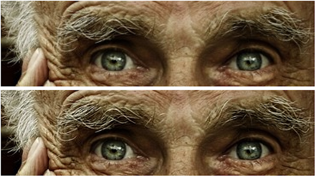
Top: Original, Bottom: RAISR super-resolved 2x
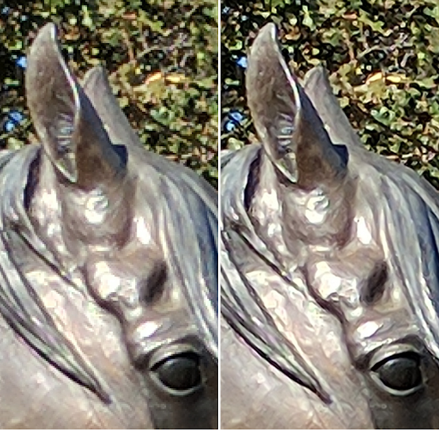
Left: Original, Right: RAISR super-resolved 3x

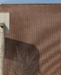
One of the more complex aspects of super-resolution is getting rid of aliasing artifacts such as Moire patterns and jaggies that arise when high frequency content is rendered in lower resolution (as is the case when images are purposefully degraded). Depending on the shape of the underlying features, these artifacts can be varied and hard to undo.
Example of aliasing artifacts seen on the lower right (Image source)

Linear methods simply can not recover the underlying structure, but RAISR can. Below is an example where the aliased spatial frequencies are apparent under the numbers 3 and 5 in the low-resolution original on the left, while the RAISR image on the right recovered the original structure. Another important advantage of the filter learning approach used by RAISR is that we can specialize it to remove noise, or compression artifacts unique to individual compression algorithms (such as JPEG) as part of the training process. By providing it with examples of such artifacts, RAISR can learn to undo other effects besides resolution enhancement, having them “baked” inside the resulting filters.
Left: Low res original, with strong aliasing. Right: RAISR output, removing aliasing.

Super-resolution technology, using one or many frames, has come a long way. Today, the use of machine learning, in tandem with decades of advances in imaging technology, has enabled progress in image processing that yields many potential benefits. For example, in addition to improving digital “pinch to zoom” on your phone, one could capture, save, or transmit images at lower resolution and super-resolve on demand without any visible degradation in quality, all while utilizing less of mobile data and storage plans.

To learn more about the details of our research and a comparison to other current architectures, check out our paper, which will appear soon in the IEEE Transactions on Computational Imaging.


Motion Stills – Create beautiful GIFs from Live Photos


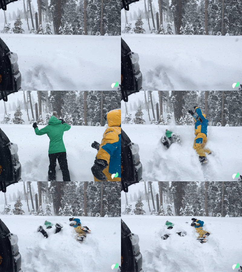
Today we are releasing Motion Stills, an iOS app from Google Research that acts as a virtual camera operator for your Apple Live Photos. We use our video stabilization technology to freeze the background into a still photo or create sweeping cinematic pans. The resulting looping GIFs and movies come alive, and can easily be shared via messaging or on social media.
With Motion Stills, we provide an immersive stream experience that makes your clips fun to watch and share. You can also tell stories of your adventures by combining multiple clips into a movie montage. All of this works right on your phone, no Internet connection needed.
A Live Photo before and after stabilization with Motion Stills
How does it work?
We pioneered this technology by stabilizing hundreds of millions of videos and creating GIF animations from photo bursts. Our algorithm uses linear programming to compute a virtual camera path that is optimized to recast videos and bursts as if they were filmed using stabilization equipment, yielding a still background or creating cinematic pans to remove shakiness.

Our challenge was to take technology designed to run distributed in a data center and shrink it down to run even faster on your mobile phone. We achieved a 40x speedup by using techniques such as temporal subsampling, decoupling of motion parameters, and using Google Research’s custom linear solver, GLOP. We obtain further speedup and conserve storage by computing low-resolution warp textures to perform real-time GPU rendering, just like in a videogame.
Making it loop
Short videos are perfect for creating loops, so we added loop optimization to bring out the best in your captures. Our approach identifies optimal start and end points, and also discards blurry frames. As an added benefit, this fixes “pocket shots” (footage of the phone being put back into the pocket).

To keep the background steady while looping, Motion Stills has to separate the background from the rest of the scene. This is a difficult task when foreground elements occlude significant portions of the video, as in the example below. Our novel method classifies motion vectors into foreground (red) and background (green) in a temporally consistent manner. We use a cascade of motion models, moving our motion estimation from simple to more complex models and biasing our results along the way.
Left: Original with virtual camera path (red rectangle) and motion classification; foreground(red) vs. background(green) Right: Motion Stills result
Try it out
We’re excited to see what you can create with this app. From fun family moments to exciting adventures with friends, try it out and let us know what you think. Motion Stills is an on-device experience with no sign-in: even if you’re on top of a glacier without signal, you can see your results immediately. You can show us your favorite clips by using #motionstill on social media.

This app is a way for us to experiment and iterate quickly on the technology needed for short video creation. Based on the feedback we receive, we hope to integrate this feature into existing products like Google Photos.

Motion Stills is available on the App Store.