Tag Archives: machine learning

Developer Journey – Women’s History Month: March 2023

Posted by Lyanne Alfaro, DevRel Program Manager, Google Developer Studio

In honor of Women’s History Month, it’s our pleasure to feature members across the Women Techmakers ecosystem for March’s Developer Journey profiles. These are community leaders who have explored, navigated and built using Google tools. They are active members of the broader Google Developers community.

In March, the WTM program will also celebrate International Women’s Day, centered on the theme “Dare To Be,” celebrating the courage and strength that this community demonstrates, made of thought leaders who are creating a world where women can thrive in tech. You can find more about the Women Techmakers program during IWD here.
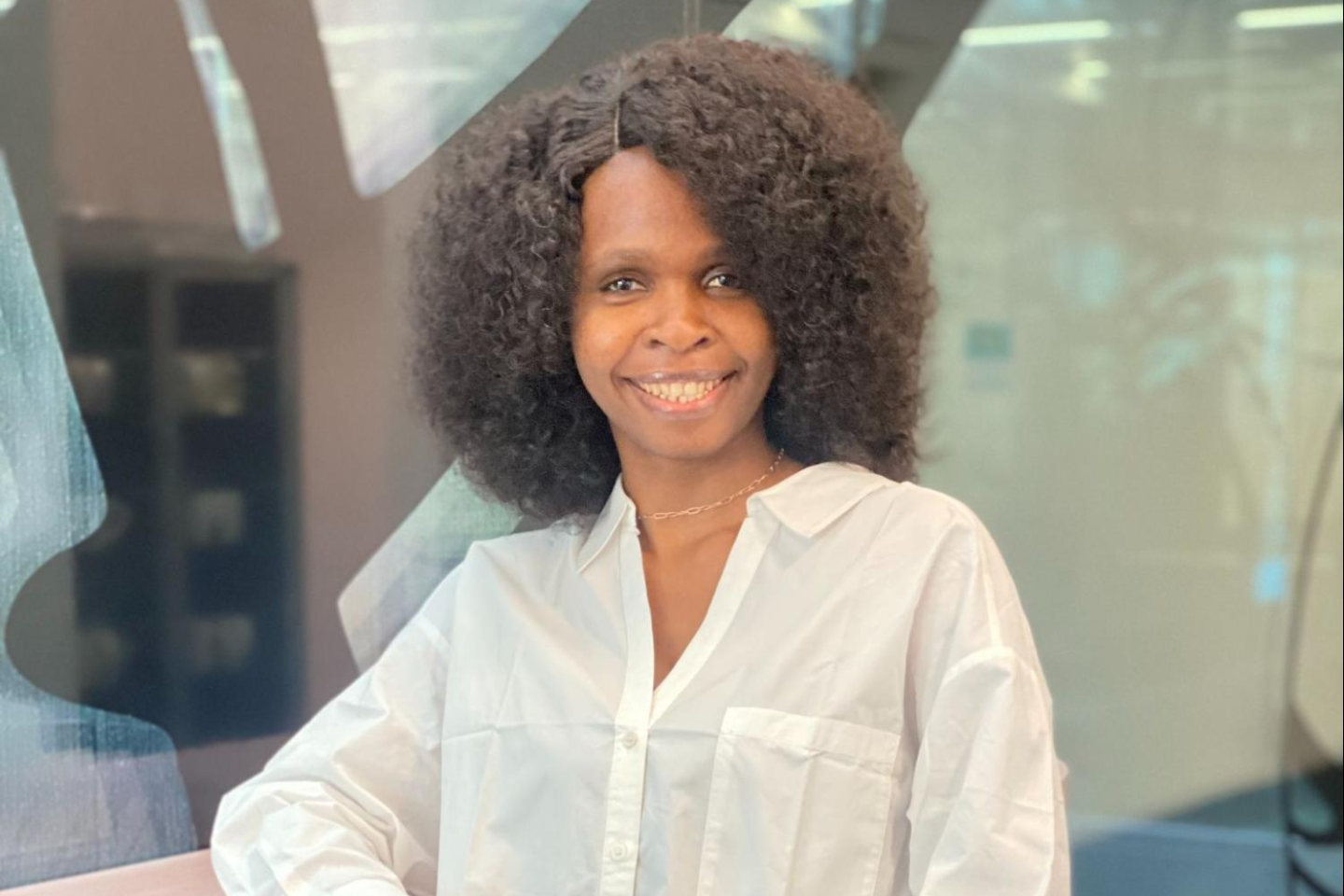

Headshot of Ezinne Osuamadi smiling

Ezinne Osuamadi

Women Techmakers Mentor and Ambassador
Waldorf, Germany (A proud Nigerian!)
Software Developer/ Technical Product Manager
Twitter
Linkedln
Instagram

What Google tools have you used to build?

Android Studio, Firebase, Google Play Services, Google Analytics. I'm a mobile developer and recently started getting my hands on technical product management and agile product owner. The tools I use for development are Android as the framework and Android Studio as the integrated development environment.

Which tool has been your favorite to use? Why?

I would say Flutter. The Flutter toolkit has a layered architecture that allows for full customization. The fact that Flutter comes with fully-customizable widgets allows you to build native interfaces in minutes. I also love the fact that some of these widgets’ features like scrolling, navigation, icons, and fonts provide a full native performance on both iOS and Android. Flutter is one code base and it makes building mobile applications much easier. I don't have to build a separate app for Android, and another separate app for IOS. Another Flutter feature I like so much is the “hot reload.” It allows me to easily build UIs, add new features, and fix bugs faster. It also allows easy compilation of Flutter code to native ARM machine code using Dart native compilers.

Please share with us about something you’ve built in the past using Google tools.

The first app I built was for one of my former employers. It happened almost three years ago, and it was the first project I worked on when I started learning Flutter. I was super excited about it. It was a timesheet app targeted specifically for employees. The sole purpose of the app is for employees to be able to schedule tasks and also give a time slot to each task.

What advice would you give someone starting in their developer journey?

From my experience running an NGO called Ladies Crushing IT Africa and organizing a couple of tech events, I would say this: Don’t go into software development if you are not passionate or interested in it. Going into development because you think they pay developers well or because your friends are earning money from it is a wrong reason to start your development journey. A tech career journey should be about what you want to be in the future. Does it align with your future goals and objectives? How or what are strategies in achieving that path? Also note that the path to becoming a successful developer is a process. It is not all roses, and there are times when debugging will make it look difficult. But you should be resilient and diligent in making the most out of it when you encounter difficulties. It is always about continuous improvement. Never stop learning to keep yourself up to date with latest technologies and development tools.
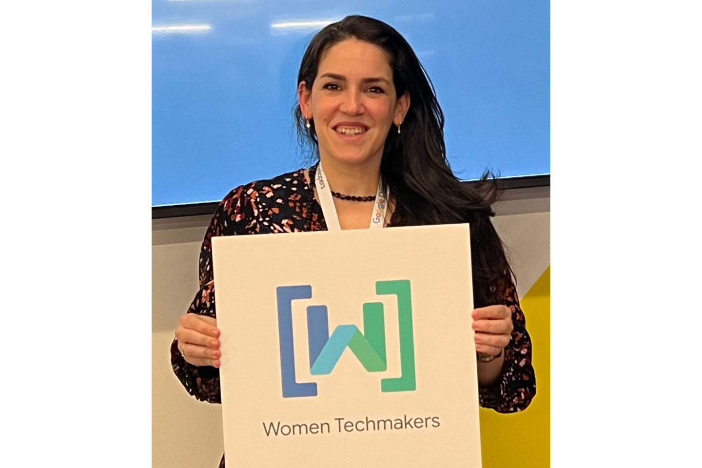
 

Headshot of Patty O’Callaghan smiling

Patty O’Callaghan

GDG Glasgow and Women Techmakers Ambassador
Glasgow, Scotland
Tech Lead @ Charles River Laboratories
Twitter
Linkedln

What Google tools have you used to build?

I use the Chrome DevTools daily. I find them very helpful. I also enjoy working on projects using TensorFlow.JS and Firebase.

Which tool has been your favorite to use? Why?

I would have to say TensorFlow.JS and its pre-made models are my favorite. I enjoy the fact that I can build cool machine learning projects directly in the browser. Even developers unfamiliar with this technology can quickly build, train, and deploy machine learning models using just a few lines of code. Some kids at my code club have used TensorFlow.JS for amazing projects, like building class attendance applications using facial recognition, or a site that checks correct form while practicing karate at home, and another for studying with the help of an AI agent.

Please share with us about something you’ve built in the past using Google tools.

I've worked on several side-projects using TensorFlow.JS for my workshops. One of my favorites is an emotion recognition app, using the Teachable Machine. Additionally, for work, I used TF.JS to develop a machine learning solution that suggests taxonomies for articles based on their content. It analyzes over 30 taxonomies to find the best match for the given article.

What advice would you give someone starting in their developer journey?

First of all, focus on learning the fundamentals of programming. A strong foundation will benefit you in the long run. Practice coding regularly and find a mentor or a community to help you along the way. For example, contributing to an open-source project is an excellent way to learn. And remember: Making mistakes is a natural part of the learning process, so don't get discouraged if you encounter difficulties. Keep pushing forward!


Headshot of Alexis and David Snelling smiling

Alexis & David Snelling

Alexis – Women Techmakers Ambassador & Lead
Named as Top 10 Women founders to Watch in 2023 by Forbes Group
San Francisco, CA
CEO WeTransact.live
Twitter
Linkedln
Facebook
 

David – Google Developer Groups
San Francisco, CA
CTO WeTransact.live
Twitter
Linkedln
Facebook

What Google tools have you used to build?

Here’s just a few of the tools we’ve used:
  • Angular 15
  • Material Design
  • Google Cloud / Firebase
    • Authentication
    • Hosting
    • Firestore
    • Functions
    • Extensions
    • Storage
    • Machine Learning
  • PWA Standards
  • Chrome / DevTools
  • Android

Which tool has been your favorite to use? Why?

Firestore has been our favorite due to its scalability and real-time data capabilities, through websockets and triggers, the data flexibility, plus query capabilities. This is how we’ve built out our modern event-driven architecture to allow for a completely real-time application providing immediate data and collaboration across our entire white label application suite.

Please share with us about something you’ve built in the past using Google tools.

We built the WeTransact Innovation Platform: From Idea to ROI which offers a learning-based distributed social platform for learning, collaborating and presenting yourself and your innovations.

For customers, we’ve created a White Label SaaS Platform, licensed by universities, incubators, developer groups and any program looking to provide education, collaboration, and AI assisted auto generated presentation and communication tools. Our platform combines features similar to LinkedIn, Coursera, AngelList and Zoom in one simple and modern unified platform for communities to make collaboration & lifelong learning globally accessible to everyone. The WeTransact platform accelerates & scales your program’s impact to solve the world's biggest problems better together.

Here’s just a few other ways we’ve used Google tools:

What advice would you give someone starting in their developer journey?

There’s a few pieces of advice we’d offer! Among them is to start early. Find a friend who is already developing or shares your passion. Find an open source project that inspires you or represents something you're passionate about. Dig in, change stuff, break stuff and then learn why. Search is your best friend – use it to always question and reset your assumptions, learn new approaches, and practice not getting stuck in a “boilerplate” or “standard” solution to each problem. It’s not about memorizing – technology changes every day and you should too. Finally, know that it’s about the process and the journey, not the destination.

ML Olympiad 2023: Globally Distributed ML Competitions by Google ML Community

Posted by Hee Jung, DevRel Community Manager

What is the ML Olympiad?

The ML Olympiad is an associated Kaggle Community Competitions hosted by ML GDE, TFUG, 3rd-party ML communities, supported by Google Developers. The ML Developer Programs team and the communities successfully ran the first round of the campaign in 2022 and are now launching the second round. The goal of this campaign is to provide ML training opportunities for developers by leveraging Kaggle’s features.

ML Olympiad Community Competitions

17 ML Olympiad community competitions are currently open. Visit the ML Olympiad page to participate.

Into the Space

  • Predicting which spaceship passengers were transported by the anomaly using records recovered from the spaceship’s damaged computer system.
  • Host: MD Shahriyar Al Mustakim Mitul / TFUG Dhaka

    Water Quality Prediction

    • Estimating the quality of water.
    • Hosts: Usha Rengaraju, Vijayabharathi Karuppasamy (TFUG Chennai), Samuel T (TFUG Mysuru)

      Breast Cancer Diagnosis

      • Predicting medical diagnosis [breast cancer].
      • Host: Ankit Kumar Verma / TFUG Prayagraj

        Book Recommendations

        • To provide personalized recommendations to users based on their reading history and preferences using various machine learning algorithms.
        • Hosts: Anushka Raj, Yugandhar Surya / TFUG Hajipur

          Argania Tree Deforestation Detection

          • Use Sentinel-2 satellite imagery to detect and map areas of deforestation in the Argania region.
          • Hosts: Taha Bouhsine / TFUG Agadir

            Multilingual Spell Correction

            • Reconstruct noisy sentences in European languages: English, French, German, Bulgarian and Turkish.
            • Host: Radostin Cholakov (ML GDE)

              CO2 Emissions Forecasting

              • Forecasting CO2 emissions based on deforestation in Côte d'Ivoire.
              • Hosts: Armel Yara, Kimana Misago, Jordan Erifried / TFUG Abidjan

                Ensure Healthy Lives (in local language) 

                • Use ML techniques to help achieve common good health and well-being.
                • Hosts: Vinicius Fernandes Caridá (ML GDE), Pedro Gengo, Alex Fernandes Mansano / TFUG São Paulo

                  Predictive Maintenance

                  • Predict future engine’s failures.
                  • Host: Daniel Pereda / TFUG Santiago

                    Firetrucks Are Red And Cars Are Blue

                    • To create a model that can accurately predict the correct class for each image, without overfitting.
                    • Host: Prasoon Kottarathil / TFUG Thrissur

                      Dialect Recognition (in Arabic) 

                      • Dialect recognition in order to improve user experience in AI applications.
                      • Hosts: Ruqiya Bin Safi (ML GDE), Eyad Sibai, Hussain Alfayez / Saudi TFUG & Applied ML/AI group

                        Sentiment Analysis Of JUMIA Tunisia  (in local language) 

                        • Use JUMIA customer reviews to determine the sentiment of content from text data.
                        • Host: Boulbaba BEN AMMAR / TFUG Sfax

                          Kolkata Housing Prediction

                          • Kolkata housing prediction results can be used to address related social and economic issues.
                          • Host: Rishiraj Acharya / TFUG Kolkata

                            Can You Guess The Beer Style?

                            • This is a machine learning competition focused on classifying beer into 17 distinct styles based on key descriptors.
                            • Host: Marvik

                              Detect ChatGpt answers

                              • The goal of this competition is to classify ChatGpt answers vs real human answers for a variety of questions.
                              • Host: Elyes Manai (ML GDE) / IEEE ESSTHS + GDSC ISETSO + PyData Tunisia

                                MLAct Pose Detection

                                • Raising awareness about some basic yoga poses, and encouraging our community members to practice the basic parts of computer vision.
                                • Host: Imen Masmoudi / MLAct ML Community

                                  Hausa Sentiment Analysis 2.0 (in local language) 

                                  • Classify the sentiment of sentences of Hausa Language.
                                  • Hosts: Nuruddeen Sambo, Dattijo Murtala Makama / TFUG Bauchi

                                    Navigating ML Olympiad

                                    You can search “ML Olympiad” on Kaggle Community Competitions page to see them all. And for further info, look for #MLOlympiad on social media.

                                    Google Developers supports the hosts of each competition. Browse through the available competitions and participate in those that interest you!

                                    Real-time tracking of wildfire boundaries using satellite imagery

                                    As global temperatures rise, wildfires around the world are becoming more frequent and more dangerous. Their effects are felt by many communities as people evacuate their homes or suffer harm even from proximity to the fire and smoke.

                                    As part of Google’s mission to help people access trusted information in critical moments, we use satellite imagery and machine learning (ML) to track wildfires and inform affected communities. Our wildfire tracker was recently expanded. It provides updated fire boundary information every 10–15 minutes, is more accurate than similar satellite products, and improves on our previous work. These boundaries are shown for large fires in the continental US, Mexico, and most of Canada and Australia. They are displayed, with additional information from local authorities, on Google Search and Google Maps, allowing people to keep safe and stay informed about potential dangers near them, their homes or loved ones.

                                    Real-time boundary tracking of the 2021-2022 Wrattonbully bushfire, shown as a red polygon in Google Maps.

                                    Inputs

                                    Wildfire boundary tracking requires balancing spatial resolution and update frequency. The most scalable method to obtain frequent boundary updates is to use geostationary satellites, i.e., satellites that orbit the earth once every 24 hours. These satellites remain at a fixed point above Earth, providing continual coverage of the area surrounding that point. Specifically, our wildfire tracker models use the GOES-16 and GOES-18 satellites to cover North America, and the Himawari-9 and GK2A satellites to cover Australia. These provide continent-scale images every 10 minutes. The spatial resolution is 2km at nadir (the point directly below the satellite), and lower as one moves away from nadir. The goal here is to provide people with warnings as soon as possible, and refer them to authoritative sources for spatially precise, on-the-ground data, as necessary.

                                    Smoke plumes obscuring the 2018 Camp Fire in California. [Image from NASA Worldview]

                                    Determining the precise extent of a wildfire is nontrivial, since fires emit massive smoke plumes, which can spread far from the burn area and obscure the flames. Clouds and other meteorological phenomena further obscure the underlying fire. To overcome these challenges, it is common to rely on infrared (IR) frequencies, particularly in the 3–4 μm wavelength range. This is because wildfires (and similar hot surfaces) radiate considerably at this frequency band, and these emissions diffract with relatively minor distortions through smoke and other particulates in the atmosphere. This is illustrated in the figure below, which shows a multispectral image of a wildfire in Australia. The visible channels (blue, green, and red) mostly show the triangular smoke plume, while the 3.85 μm IR channel shows the ring-shaped burn pattern of the fire itself. Even with the added information from the IR bands, however, determining the exact extent of the fire remains challenging, as the fire has variable emission strength, and multiple other phenomena emit or reflect IR radiation.

                                    Himawari-8 hyperspectral image of a wildfire. Note the smoke plume in the visible channels (blue, green, and red), and the ring indicating the current burn area in the 3.85μm band.

                                    Model

                                    Prior work on fire detection from satellite imagery is typically based on physics-based algorithms for identifying hotspots from multispectral imagery. For example, the National Oceanic and Atmospheric Administration (NOAA) fire product identifies potential wildfire pixels in each of the GOES satellites, primarily by relying on the 3.9 μm and 11.2 μm frequencies (with auxiliary information from two other frequency bands).

                                    In our wildfire tracker, the model is trained on all satellite inputs, allowing it to learn the relative importance of different frequency bands. The model receives a sequence of the three most recent images from each band so as to compensate for temporary obstructions such as cloud cover. Additionally, the model receives inputs from two geostationary satellites, achieving a super-resolution effect whereby the detection accuracy improves upon the pixel size of either satellite. In North America, we also supply the aforementioned NOAA fire product as input. Finally, we compute the relative angles of the sun and the satellites, and provide these as additional input to the model.

                                    All inputs are resampled to a uniform 1 km–square grid and fed into a convolutional neural network (CNN). We experimented with several architectures and settled on a CNN followed by a 1x1 convolutional layer to yield separate classification heads for fire and cloud pixels (shown below). The number of layers and their sizes are hyperparameters, which are optimized separately for Australia and North America. When a pixel is identified as a cloud, we override any fire detection since heavy clouds obscure underlying fires. Even so, separating the cloud classification task improves the performance of fire detection as we incentivize the system to better identify these edge cases.

                                    CNN architecture for the Australia model; a similar architecture was used for North America. Adding a cloud classification head improves fire classification performance.

                                    To train the network, we used thermal anomalies data from the MODIS and VIIRS polar-orbiting satellites as labels. MODIS and VIIRS have higher spatial accuracy (750–1000 meters) than the geostationary satellites we use as inputs. However, they cover a given location only once every few hours, which occasionally causes them to miss rapidly-advancing fires. Therefore, we use MODIS and VIIRS to construct a training set, but at inference time we rely on the high-frequency imagery from geostationary satellites.

                                    Even when limiting attention to active fires, most pixels in an image are not currently burning. To reduce the model's bias towards non-burning pixels, we upsampled fire pixels in the training set and applied focal loss to encourage improvements in the rare misclassified fire pixels.

                                    The progressing boundary of the 2022 McKinney fire, and a smaller nearby fire.

                                    Evaluation

                                    High-resolution fire signals from polar-orbiting satellites are a plentiful source for training data. However, such satellites use sensors that are similar to geostationary satellites, which increases the risk of systemic labeling errors (e.g., cloud-related misdetections) being incorporated into the model. To evaluate our wildfire tracker model without such bias, we compared it against fire scars (i.e., the shape of the total burnt area) measured by local authorities. Fire scars are obtained after a fire has been contained and are more reliable than real-time fire detection techniques. We compare each fire scar to the union of all fire pixels detected in real time during the wildfire to obtain an image such as the one shown below. In this image, green represents correctly identified burn areas (true positive), yellow represents unburned areas detected as burn areas (false positive), and red represents burn areas that were not detected (false negative).

                                    Example evaluation for a single fire. Pixel size is 1km x 1km.

                                    We compare our models to official fire scars using the precision and recall metrics. To quantify the spatial severity of classification errors, we take the maximum distance between a false positive or false negative pixel and the nearest true positive fire pixel. We then average each metric across all fires. The results of the evaluation are summarized below. Most severe misdetections were found to be a result of errors in the official data, such as a missing scar for a nearby fire.

                                    Test set metrics comparing our models to official fire scars.

                                    We performed two additional experiments on wildfires in the United States (see table below). First, we evaluated an earlier model that relies only on NOAA's GOES-16 and GOES-17 fire products. Our model outperforms this approach in all metrics considered, demonstrating that the raw satellite measurements can be used to enhance the existing NOAA fire product.

                                    Next, we collected a new test set consisting of all large fires in the United States in 2022. This test set was not available during training because the model launched before the fire season began. Evaluating the performance on this test set shows performance in line with expectations from the original test set.

                                    Comparison between models on fires in the United States.


                                    Conclusion

                                    Boundary tracking is part of Google’s wider commitment to bring accurate and up-to-date information to people in critical moments. This demonstrates how we use satellite imagery and ML to track wildfires, and provide real time support to affected people in times of crisis. In the future, we plan to keep improving the quality of our wildfire boundary tracking, to expand this service to more countries and continue our work helping fire authorities access critical information in real time.


                                    Acknowledgements

                                    This work is a collaboration between teams from Google Research, Google Maps and Crisis Response, with support from our partnerships and policy teams. We would also like to thank the fire authorities whom we partner with around the world.


                                    Source: Google AI Blog


                                    The Flan Collection: Advancing open source methods for instruction tuning

                                    Language models are now capable of performing many new natural language processing (NLP) tasks by reading instructions, often that they hadn’t seen before. The ability to reason on new tasks is mostly credited to training models on a wide variety of unique instructions, known as “instruction tuning”, which was introduced by FLAN and extended in T0, Super-Natural Instructions, MetaICL, and InstructGPT. However, much of the data that drives these advances remain unreleased to the broader research community. 

                                    In “The Flan Collection: Designing Data and Methods for Effective Instruction Tuning”, we closely examine and release a newer and more extensive publicly available collection of tasks, templates, and methods for instruction tuning to advance the community’s ability to analyze and improve instruction-tuning methods. This collection was first used in Flan-T5 and Flan-PaLM, for which the latter achieved significant improvements over PaLM. We show that training a model on this collection yields improved performance over comparable public collections on all tested evaluation benchmarks, e.g., a 3%+ improvement on the 57 tasks in the Massive Multitask Language Understanding (MMLU) evaluation suite and 8% improvement on BigBench Hard (BBH). Analysis suggests the improvements stem both from the larger and more diverse set of tasks and from applying a set of simple training and data augmentation techniques that are cheap and easy to implement: mixing zero-shot, few-shot, and chain of thought prompts at training, enriching tasks with input inversion, and balancing task mixtures. Together, these methods enable the resulting language models to reason more competently over arbitrary tasks, even those for which it hasn’t seen any fine-tuning examples. We hope making these findings and resources publicly available will accelerate research into more powerful and general-purpose language models.


                                    Public instruction tuning data collections

                                    Since 2020, several instruction tuning task collections have been released in rapid succession, shown in the timeline below. Recent research has yet to coalesce around a unified set of techniques, with different sets of tasks, model sizes, and input formats all represented. This new collection, referred to below as “Flan 2022”, combines prior collections from FLAN, P3/T0, and Natural Instructions with new dialog, program synthesis, and complex reasoning tasks.

                                    A timeline of public instruction tuning collections, including: UnifiedQA, CrossFit, Natural Instructions, FLAN, P3/T0, MetaICL, ExT5, Super-Natural Instructions, mT0, Unnatural Instructions, Self-Instruct, and OPT-IML Bench. The table describes the release date, the task collection name, the model name, the base model(s) that were finetuned with this collection, the model size, whether the resulting model is Public (green) or Not Public (red), whether they train with zero-shot prompts (“ZS”), few-shot prompts (“FS”), chain-of-thought prompts (“CoT”) together (“+”) or separately (“/”), the number of tasks from this collection in Flan 2022, the total number of examples, and some notable methods, related to the collections, used in these works. Note that the number of tasks and examples vary under different assumptions and so are approximations. Counts for each are reported using task definitions from the respective works.

                                    In addition to scaling to more instructive training tasks, The Flan Collection combines training with different types of input-output specifications, including just instructions (zero-shot prompting), instructions with examples of the task (few-shot prompting), and instructions that ask for an explanation with the answer (chain of thought prompting). Except for InstructGPT, which leverages a collection of proprietary data, Flan 2022 is the first work to publicly demonstrate the strong benefits of mixing these prompting settings together during training. Instead of a trade-off between the various settings, mixing prompting settings during training improves all prompting settings at inference time, as shown below for both tasks held-in and held-out from the set of fine-tuning tasks.

                                    Training jointly with zero-shot and few-shot prompt templates improves performance on both held-in and held-out tasks. The stars indicate the peak performance in each setting. Red lines denote the zero-shot prompted evaluation, lilac denotes few-shot prompted evaluation.

                                    Evaluating instruction tuning methods

                                    To understand the overall effects of swapping one instruction tuning collection for another, we fine-tune equivalently-sized T5 models on popular public instruction-tuning collections, including Flan 2021, T0++, and Super-Natural Instructions. Each model is then evaluated on a set of tasks that are already included in each of the instruction tuning collections, a set of five chain-of-thought tasks, and then a set of 57 diverse tasks from the MMLU benchmark, both with zero-shot and few-shot prompts. In each case, the new Flan 2022 model, Flan-T5, outperforms these prior works, demonstrating a more powerful general-purpose NLP reasoner.

                                    Comparing public instruction tuning collections on held-in, chain-of-thought, and held-out evaluation suites, such as BigBench Hard and MMLU. All models except OPT-IML-Max (175B) are trained by us, using T5-XL with 3B parameters. Green text indicates improvement over the next best comparable T5-XL (3B) model.

                                    Single task fine-tuning

                                    In applied settings, practitioners usually deploy NLP models fine-tuned specifically for one target task, where training data is already available. We examine this setting to understand how Flan-T5 compares to T5 models as a starting point for applied practitioners. Three settings are compared: fine-tuning T5 directly on the target task, using Flan-T5 without further fine-tuning on the target task, and fine-tuning Flan-T5 on the target task. For both held-in and held-out tasks, fine-tuning Flan-T5 offers an improvement over fine-tuning T5 directly. In some instances, usually where training data is limited for a target task, Flan-T5 without further fine-tuning outperforms T5 with direct fine-tuning.

                                    Flan-T5 outperforms T5 on single-task fine-tuning. We compare single-task fine-tuned T5 (blue bars), single-task fine-tuned Flan-T5 (red), and Flan-T5 without any further fine-tuning (beige).

                                    An additional benefit of using Flan-T5 as a starting point is that training is significantly faster and cheaper, converging more quickly than T5 fine-tuning, and usually peaking at higher accuracies. This suggests less task-specific training data may be necessary to achieve similar or better results on a particular task.

                                    Flan-T5 converges faster than T5 on single-task fine-tuning, for each of five held-out tasks from Flan fine-tuning. Flan-T5’s learning curve is indicated with the solid lines, and T5’s learning curve with the dashed line. All tasks are held-out during Flan finetuning.

                                    There are significant energy efficiency benefits for the NLP community to adopt instruction-tuned models like Flan-T5 for single task fine-tuning, rather than conventional non-instruction-tuned models. While pre-training and instruction fine-tuning are financially and computationally expensive, they are a one-time cost, usually amortized over millions of subsequent fine-tuning runs, which can become more costly in aggregate, for the most prominent models. Instruction-tuned models offer a promising solution in significantly reducing the amount of fine-tuning steps needed to achieve the same or better performance.


                                    Conclusion

                                    The new Flan instruction tuning collection unifies the most popular prior public collections and their methods, while adding new templates and simple improvements like training with mixed prompt settings. The resulting method outperforms Flan, P3, and Super-Natural Instructions on held-in, chain of thought, MMLU, and BBH benchmarks by 3–17% across zero-shot and few-shot variants. Results suggest this new collection serves as a more performant starting point for researchers and practitioners interested in both generalizing to new instructions or fine-tuning on a single new task.


                                    Acknowledgements

                                    It was a privilege to work with Jason Wei, Barret Zoph, Le Hou, Hyung Won Chung, Tu Vu, Albert Webson, Denny Zhou, and Quoc V Le on this project.

                                    Source: Google AI Blog


                                    Machine Learning Communities: Q4 ‘22 highlights and achievements

                                    Posted by Nari Yoon, Hee Jung, DevRel Community Manager / Soonson Kwon, DevRel Program Manager

                                    Let’s explore highlights and accomplishments of vast Google Machine Learning communities over the last quarter of 2022. We are enthusiastic and grateful about all the activities by the global network of ML communities. Here are the highlights!


                                    ML at DevFest 2022

                                    A group of ML Developers attending DevFest 2022

                                    A large number of members of ML GDE, TFUG, and 3P ML communities participated in DevFests 2022 worldwide covering various ML topics with Google products. Machine Learning with Jax: Zero to Hero (DevFest Conakry) by ML GDE Yannick Serge Obam Akou (Cameroon) and Easy ML on Google Cloud (DevFest Med) by ML GDE Nathaly Alarcon Torrico (Bolivia) hosted great sessions.

                                    ML Community Summit 2022

                                    A group of ML Developers attending ML Community Summit

                                    ML Community Summit 2022 was hosted on Oct 22-23, 2022, in Bangkok, Thailand. Twenty-five most active community members (ML GDE or TFUG organizer) were invited and shared their past activities and thoughts on Google’s ML products. A video sketch from ML Developer Programs team and a blog posting by ML GDE Margaret Maynard-Reid (United States) help us revisit the moments.

                                    TensorFlow

                                    MAXIM in TensorFlow by ML GDE Sayak Paul (India) shows his implementation of the MAXIM family of models in TensorFlow.

                                    Diagram of gMLP block

                                    gMLP: What it is and how to use it in practice with Tensorflow and Keras? by ML GDE Radostin Cholakov (Bulgaria) demonstrates the state-of-the-art results on NLP and computer vision tasks using a lot less trainable parameters than corresponding Transformer models. He also wrote Differentiable discrete sampling in TensorFlow.

                                    Building Computer Vision Model using TensorFlow: Part 2 by TFUG Pune for the developers who want to deep dive into training an object detection model on Google Colab, inspecting the TF Lite model, and deploying the model on an Android application. ML GDE Nitin Tiwari (India) covered detailed aspects for end-to-end training and deployment of object model detection.

                                    Advent of Code 2022 in pure TensorFlow (days 1-5) by ML GDE Paolo Galeone (Italy) solving the Advent of Code (AoC) puzzles using only TensorFlow. The articles contain a description of the solutions of the Advent of Code puzzles 1-5, in pure TensorFlow.

                                    tf.keras.metrics / tf.keras.optimizers by TFUG Taipei helped people learn the TF libraries. They shared basic concepts and how to use them using Colab.

                                    Screen shot of TensorFlow Lite on Android Project Practical Course
                                    A hands-on course on TensorFlow Lite projects on Android by ML GDE Xiaoxing Wang (China) is the book mainly introducing the application of TensorFlow Lite in Android development. The content focuses on applying three typical ML applications in Android development.

                                    Build tensorflow-lite-select-tf-ops.aar and tensorflow-lite.aar files with Colab by ML GDE George Soloupis (Greece) guides how you can shrink the final size of your Android application’s .apk by building tensorflow-lite-select-tf-ops.aar and tensorflow-lite.aar files without the need of Docker or personal PC environment.

                                    TensorFlow Lite and MediaPipe Application by ML GDE XuHua Hu (China) explains how to use TFLite to deploy an ML model into an application on devices. He shared experiences with developing a motion sensing game with MediaPipe, and how to solve problems that we may meet usually.

                                    Train and Deploy TensorFlow models in Go by ML GDE Paolo Galeone (Italy) delivered the basics of the TensorFlow Go bindings, the limitations, and how the tfgo library simplifies their usage.

                                    Keras

                                    Diagram of feature maps concatenated together and flattened

                                    Complete Guide on Deep Learning Architectures, Chapter 1 on ConvNets by ML GDE Merve Noyan (France) brings you into the theory of ConvNets and shows how it works with Keras.

                                    Hazy Image Restoration Using Keras by ML GDE Soumik Rakshit (India) provides an introduction to building an image restoration model using TensorFlow, Keras, and Weights & Biases. He also shared an article Improving Generative Images with Instructions: Prompt-to-Prompt Image Editing with Cross Attention Control.

                                    Mixed precision in Keras based Stable Diffusion
                                    Let’s Generate Images with Keras based Stable Diffusion by ML GDE Chansung Park (Korea) delivered how to generate images with given text and what stable diffusion is. He also talked about Keras-based stable diffusion, basic building blocks, and the advantages of using Keras-based stable diffusion.

                                    A Deep Dive into Transformers with TensorFlow and Keras: Part 1, Part 2, Part3 by ML GDE Aritra Roy Gosthipaty (India) covered the journey from the intuition of attention to formulating the multi-head self-attention. And TensorFlow port of GroupViT in 🤗 transformers library was his contribution to Hugging Face transformers library.

                                    TFX

                                    Digits + TFX banner

                                    How startups can benefit from TFX by ML GDE Hannes Hapke (United States) explains how the San Francisco-based FinTech startup Digits has benefitted from applying TFX early, how TFX helps Digits grow, and how other startups can benefit from TFX too.

                                    Usha Rengaraju (India) shared TensorFlow Extended (TFX) Tutorials (Part 1, Part 2, Part 3) and the following TF projects: TensorFlow Decision Forests Tutorial and FT Transformer TensorFlow Implementation.

                                    Hyperparameter Tuning and ML Pipeline by ML GDE Chansung Park (Korea) explained hyperparam tuning, why it is important; Introduction to KerasTuner, basic usage; how to visualize hyperparam tuning results with TensorBoard; and integration within ML pipeline with TFX.

                                    JAX/Flax

                                    JAX High-performance ML Research by TFUG Taipei and ML GDE Jerry Wu (Taiwan) introduced JAX and how to start using JAX to solve machine learning problems.

                                    [TensorFlow + TPU] GatedTabTransformer[W&B] and its JAX/Flax counterpart GatedTabTransformer-FLAX[W&B] by Usha Rengaraju (India) are tutorial series containing the implementation of GatedTabTransformer paper in both TensorFlow (TPU) and FLAX.

                                    Putting NeRF on a diet: Semantically consistent Few-Shot View Synthesis Implementation
                                    JAX implementation of Diet NeRf by ML GDE Wan Hong Lau (Singapore) implemented the paper “Putting NeRF on a Diet (DietNeRF)” in JAX/Flax. And he also implemented a JAX-and-Flax training pipeline with the ResNet model in his Kaggle notebook, 🐳HappyWhale🔥Flax/JAX⚡TPU&GPU - ResNet Baseline.

                                    Introduction to JAX with Flax (slides) by ML GDE Phillip Lippe (Netherlands) reviewed from the basics of the requirements we have on a DL framework to what JAX has to offer. Further, he focused on the powerful function-oriented view JAX offers and how Flax allows you to use them in training neural networks.

                                    Screen grab of ML GDE David Cardozo and Cristian Garcia during a live coding session of a review of new features, specifically Shared Arrays, in the recent release of JAX
                                    JAX Streams: Exploring JAX 0.4 by ML GDE David Cardozo (Canada) and Cristian Garcia (Colombia) showed a review of new features (specifically Shared Arrays) in the recent release of JAX and demonstrated live coding.

                                    [LiveCoding] Train ResNet/MNIST with JAX/Flax by ML GDE Qinghua Duan (China) demonstrated how to train ResNet using JAX by writing code online.

                                    Kaggle

                                    Low-light Image Enhancement using MirNetv2 by ML GDE Soumik Rakshit (India) demonstrated the task of Low-light Image Enhancement.

                                    Heart disease Prediction and Diabetes Prediction Competition hosted by TFUG Chandigarh were to familiarize participants with ML problems and find solutions using classification techniques.

                                    TensorFlow User Group Bangalore Sentiment Analysis Kaggle Competition 1
                                    TFUG Bangalore Kaggle Competition - Sentiment Analysis hosted by TFUG Bangalore was to find the best sentiment analysis algorithm. Participants were given a set of training data and asked to submit an ML/DL algorithm that could predict the sentiment of a text. The group also hosted Kaggle Challenge Finale + Vertex AI Session to support the participants and guide them in learning how to use Vertex AI in a workflow.

                                    Cloud AI

                                    Better Hardware Provisioning for ML Experiments on GCP by ML GDE Sayak Paul (India) discussed the pain points of provisioning hardware (especially for ML experiments) and how we can get better provision hardware with code using Vertex AI Workbench instances and Terraform.

                                    Jayesh Sharma, Platform Engineer, Zen ML; MLOps workshop with TensorFlow and Vertex AI November 12, 2022|TensorFlow User Group Chennai
                                    MLOps workshop with TensorFlow and Vertex AI by TFUG Chennai targeted beginners and intermediate-level practitioners to give hands-on experience on the E2E MLOps pipeline with GCP. In the workshop, they shared the various stages of an ML pipeline, the top tools to build a solution, and how to design a workflow using an open-source framework like ZenML.

                                    10 Predictions on the Future of Cloud Computing by 2025: Insights from Google Next Conference by ML GDE Victor Dibia (United States) includes a recap of his notes reflecting on the top 10 cloud technology predictions discussed at the Google Cloud Next 2022 keynote.
                                    Workflow of Google Virtual Career Center
                                    O uso do Vertex AI Matching Engine no Virtual Career Center (VCC) do Google Cloud by ML GDE Rubens Zimbres (Brazil) approaches the use of Vertex AI Matching Engine as part of the Google Cloud Virtual Career Center solution.

                                    More practical time-series model with BQML by ML GDE JeongMin Kwon (Korea) introduced BQML and time-series modeling and showed some practical applications with BQML ARIMA+ and Python implementations.

                                    Vertex AI Forecast - Demand Forecasting with AutoML by ML GDE Rio Kurihara (Japan) presented a time series forecast overview, time series fusion transformers, and the benefits and desired features of AutoML.

                                    Research & Ecosystem

                                    AI in Healthcare by ML GDE Sara EL-ATEIF (Morocco) introduced AI applications in healthcare and the challenges facing AI in its adoption into the health system.

                                    Women in AI APAC finished their journey at ML Paper Reading Club. During 10 weeks, participants gained knowledge on outstanding machine learning research, learned the latest techniques, and understood the notion of “ML research” among ML engineers. See their session here.

                                    A Natural Language Understanding Model LaMDA for Dialogue Applications by ML GDE Jerry Wu (Taiwan) introduced the natural language understanding (NLU) concept and shared the operation mode of LaMDA, model fine-tuning, and measurement indicators.

                                    Python library for Arabic NLP preprocessing (Ruqia) by ML GDE Ruqiya Bin (Saudi Arabia) is her first python library to serve Arabic NLP.

                                    Screengrab of ML GDEs Margaret Maynard-Reid and Akash Nain during Chat with ML GDE Akash
                                    Chat with ML GDE Vikram & Chat with ML GDE Aakash by ML GDE Margaret Maynard-Reid (United States) shared the stories of ML GDEs’ including how they became ML GDE and how they proceeded with their ML projects.

                                    Anatomy of Capstone ML Projects 🫀by ML GDE Sayak Paul (India) discussed working on capstone ML projects that will stay with you throughout your career. He covered various topics ranging from problem selection to tightening up the technical gotchas to presentation. And in Improving as an ML Practitioner he shared his learning from experience in the field working on several aspects.

                                    Screen grab of  statement of objectives in MLOps Development Environment by ML GDE Vinicius Carida
                                    MLOps Development Environment by ML GDE Vinicius Caridá (Brazil) aims to build a full development environment where you can write your own pipelines connecting MLFLow, Airflow, GCP and Streamlit, and build amazing MLOps pipelines to practice your skills.

                                    Transcending Scaling Laws with 0.1% Extra Compute by ML GDE Grigory Sapunov (UK) reviewed a recent Google article on UL2R. And his posting Discovering faster matrix multiplication algorithms with reinforcement learning explained how AlphaTensor works and why it is important.

                                    Back in Person - Prompting, Instructions and the Future of Large Language Models by TFUG Singapore and ML GDE Sam Witteveen (Singapore) and Martin Andrews (Singapore). This event covered recent advances in the field of large language models (LLMs).

                                    ML for Production: The art of MLOps in TensorFlow Ecosystem with GDG Casablanca by TFUG Agadir discussed the motivation behind using MLOps and how it can help organizations automate a lot of pain points in the ML production process. It also covered the tools used in the TensorFlow ecosystem.

                                    Learning with Queried Hints

                                    In many computing applications the system needs to make decisions to serve requests that arrive in an online fashion. Consider, for instance, the example of a navigation app that responds to driver requests. In such settings there is inherent uncertainty about important aspects of the problem. For example, the preferences of the driver with respect to features of the route are often unknown and the delays of road segments can be uncertain. The field of online machine learning studies such settings and provides various techniques for decision-making problems under uncertainty.

                                    A navigation engine has to decide how to route this user’s request. The satisfaction of the user will depend on the (uncertain) congestion of the two routes and unknown preferences of the user on various features, such as how scenic, safe, etc., the route is.

                                    A very well known problem in this framework is the multi-armed bandit problem, in which the system has a set of n available options (arms) from which it is asked to choose in each round (user request), e.g., a set of precomputed alternative routes in navigation. The user’s satisfaction is measured by a reward that depends on unknown factors such as user preferences and road segment delays. An algorithm’s performance over T rounds is compared against the best fixed action in hindsight by means of the regret (the difference between the reward of the best arm and the reward obtained by the algorithm over all T rounds). In the experts variant of the multi-armed bandit problem, all rewards are observed after each round and not just the one played by the algorithm.

                                    An instance of the experts problem. The table presents the rewards obtained by following each of the 3 experts at each round = 1, 2, 3, 4. The best expert in hindsight (and hence the benchmark to compare against) is the middle one, with total reward 21. If, for example, we had selected expert 1 in the first two rounds and expert 3 in the last two rounds (recall that we need to select before observing the rewards of each round), we would have extracted reward 17, which would give a regret equal to 21 - 17 = 4.

                                    These problems have been extensively studied, and existing algorithms can achieve sublinear regret. For example, in the multi-armed bandit problem, the best existing algorithms can achieve regret that is of the order √T. However, these algorithms focus on optimizing for worst-case instances, and do not account for the abundance of available data in the real world that allows us to train machine learned models capable of aiding us in algorithm design.

                                    In “Online Learning and Bandits with Queried Hints” (presented at ITCS 2023), we show how an ML model that provides us with a weak hint can significantly improve the performance of an algorithm in bandit-like settings. Many ML models are trained accurately using relevant past data. In the routing application, for example, specific past data can be used to estimate road segment delays and past feedback from drivers can be used to learn the quality of certain routes. Models trained with such data can, in certain cases, give very accurate feedback. However, our algorithms achieve strong guarantees even when the feedback from the model is in the form of a less explicit weak hint. Specifically, we merely ask that the model predict which of two options will be better. In the navigation application this is equivalent to having the algorithm pick two routes and query an ETA model for which of the two is faster, or presenting the user with two routes with different characteristics and letting them pick the one that is best for them. By designing algorithms that leverage such a hint we can: Improve the regret of the bandits setting on an exponential scale in terms of dependence on T and improve the regret of the experts setting from order of √T to become independent of T. Specifically, our upper bound only depends on the number of experts n and is at most log(n).


                                    Algorithmic Ideas

                                    Our algorithm for the bandits setting utilizes the well known upper confidence bound (UCB) algorithm. The UCB algorithm maintains, as a score for each arm, the average reward observed on that arm so far and adds to it an optimism parameter that becomes smaller with the number of times the arm has been pulled, thus balancing between exploration and exploitation. Our algorithm applies the UCB scores on pairs of arms, mainly in an effort to utilize the available pairwise comparison model that can designate the better of two arms. Each pair of arms i and j is grouped as a meta-arm (i, j) whose reward in each round is equal to the maximum reward between the two arms. Our algorithm observes the UCB scores of the meta-arms and picks the pair (i, j) that has the highest score. The pair of arms are then passed as a query to the ML auxiliary pairwise prediction model, which responds with the best of the two arms. This response is the arm that is finally used by the algorithm.

                                    The decision problem considers three candidate routes. Our algorithm instead considers all pairs of the candidate routes. Suppose pair 2 is the one with the highest score in the current round. The pair is given to the auxiliary ML pairwise prediction model, which outputs whichever of the two routes is better in the current round.

                                    Our algorithm for the experts setting takes a follow-the-regularized-leader (FtRL) approach, which maintains the total reward of each expert and adds random noise to each, before picking the best for the current round. Our algorithm repeats this process twice, drawing random noise two times and picking the highest reward expert in each of the two iterations. The two selected experts are then used to query the auxiliary ML model. The model’s response for the best between the two experts is the one played by the algorithm.


                                    Results

                                    Our algorithms utilize the concept of weak hints to achieve strong improvements in terms of theoretical guarantees, including an exponential improvement in the dependence of regret on the time horizon or even removing this dependence altogether. To illustrate how the algorithm can outperform existing baseline solutions, we present a setting where 1 of the n candidate arms is consistently marginally better than the n-1 remaining arms. We compare our ML probing algorithm against a baseline that uses the standard UCB algorithm to pick the two arms to submit to the pairwise comparison model. We observe that the UCB baseline keeps accumulating regret whereas the probing algorithm quickly identifies the best arm and keeps playing it, without accumulating regret.

                                    An example in which our algorithm outperforms a UCB based baseline. The instance considers n arms, one of which is always marginally better than the remaining n-1.

                                    Conclusion

                                    In this work we explore how a simple pairwise comparison ML model can provide simple hints that prove very powerful in settings such as the experts and bandits problems. In our paper we further present how these ideas apply to more complex settings such as online linear and convex optimization. We believe our model of hints can have more interesting applications in ML and combinatorial optimization problems.


                                    Acknowledgements

                                    We thank our co-authors Aditya Bhaskara (University of Utah), Sungjin Im (University of California, Merced), and Kamesh Munagala (Duke University).

                                    Source: Google AI Blog


                                    Deciphering Clinical Abbreviations with Privacy Protecting ML

                                    Today many people have digital access to their medical records, including their doctor’s clinical notes. However, clinical notes are hard to understand because of the specialized language that clinicians use, which contains unfamiliar shorthand and abbreviations. In fact, there are thousands of such abbreviations, many of which are specific to certain medical specialities and locales or can mean multiple things in different contexts. For example, a doctor might write in their clinical notes, “pt referred to pt for lbp“, which is meant to convey the statement: “Patient referred to physical therapy for low back pain.” Coming up with this translation is tough for laypeople and computers because some abbreviations are uncommon in everyday language (e.g., “lbp” means “low back pain”), and even familiar abbreviations, such as “pt” for “patient”, can have alternate meanings, such as “physical therapy.” To disambiguate between multiple meanings, the surrounding context must be considered. It’s no easy task to decipher all the meanings, and prior research suggests that expanding the shorthand and abbreviations can help patients better understand their health, diagnoses, and treatments.

                                    In “Deciphering clinical abbreviations with a privacy protecting machine learning system”, published in Nature Communications, we report our findings on a general method that deciphers clinical abbreviations in a way that is both state-of-the-art and is on-par with board certified physicians in this task. We built the model using only public data on the web that wasn't associated with any patient (i.e., no potentially sensitive data) and evaluated performance on real, de-identified notes from inpatient and outpatient clinicians from different health systems. To enable the model to generalize from web-data to notes, we created a way to algorithmically re-write large amounts of internet text to look as if it were written by a doctor (called web-scale reverse substitution), and we developed a novel inference method, (called elicitive inference).

                                    The model input is a string that may or may not contain medical abbreviations. We trained a model to output a corresponding string in which all abbreviations are simultaneously detected and expanded. If the input string does not contain an abbreviation, the model will output the original string. By Rajkomar et al used under CC BY 4.0/ Cropped from original.

                                    Rewriting Text to Include Medical Abbreviations

                                    Building a system to translate doctors’ notes would usually start with a large, representative dataset of clinical text where all abbreviations are labeled with their meanings. But no such dataset for general use by researchers exists. We therefore sought to develop an automated way to create such a dataset but without the use of any actual patient notes, which might include sensitive data. We also wanted to ensure that models trained on this data would still work well on real clinical notes from multiple hospital sites and types of care, such as both outpatient and inpatient.

                                    To do this, we referenced a dictionary of thousands of clinical abbreviations and their expansions, and found sentences on the web that contained uses of the expansions from this dictionary. We then “rewrote” those sentences by abbreviating each expansion, resulting in web data that looked like it was written by a doctor. For instance, if a website contained the phrase “patients with atrial fibrillation can have chest pain,” we would rewrite this sentence to “pts with af can have cp.” We then used the abbreviated text as input to the model, with the original text serving as the label. This approach provided us with large amounts of data to train our model to perform abbreviation expansion.

                                    The idea of “reverse substituting” the long-forms for their abbreviations was introduced in prior research, but our distributed algorithm allows us to extend the technique to large, web-sized datasets. Our algorithm, called web-scale reverse substitution (WSRS), is designed to ensure that rare terms occur more frequently and common terms are down-sampled across the public web to derive a more balanced dataset. With this data in-hand, we trained a series of large transformer-based language models to expand the web text.

                                    We generate text to train our model on the decoding task by extracting phrases from public web pages that have corresponding medical abbreviations (shaded boxes on the left) and then substituting in the appropriate abbreviations (shaded dots, right). Since some words are found much more frequently than others ("patient" more than "posterior tibialis", both of which can be abbreviated “pt”), we downsampled common expansions to derive a more balanced dataset across the thousands of abbreviations. By Rajkomar et al used under CC BY 4.0.

                                    Adapting Protein Alignment Algorithms to Unstructured Clinical Text

                                    Evaluation of these models on the particular task of abbreviation expansion is difficult. Because they produce unstructured text as output, we had to figure out which abbreviations in the input correspond to which expansion in the output. To achieve this, we created a modified version of the Needleman Wunsch algorithm, which was originally designed for divergent sequence alignment in molecular biology, to align the model input and output and extract the corresponding abbreviation-expansion pairs. Using this alignment technique, we were able to evaluate the model’s capacity to detect and expand abbreviations accurately. We evaluated Text-to-Text Transfer Transformer (T5) models of various sizes (ranging from 60 million to over 60 billion parameters) and found that larger models performed translation better than smaller models, with the biggest model achieving the best performance.


                                    Creating New Model Inference Techniques to Coax the Model

                                    However, we did find something unexpected. When we evaluated the performance on multiple external test sets from real clinical notes, we found the models would leave some abbreviations unexpanded, and for larger models, the problem of incomplete expansion was even worse. This is mainly due to the fact that while we substitute expansions on the web for their abbreviations, we have no way of handling the abbreviations that are already present. This means that the abbreviations appear in both the original and rewritten text used as respective labels and input, and the model learns not to expand them.

                                    To address this, we developed a new inference-chaining technique in which the model output is fed again as input to coax the model to make further expansions as long as the model is confident in the expansion. In technical terms, our best-performing technique, which we call elicitive inference, involves examining the outputs from a beam search above a certain log-likelihood threshold. Using elicitive inference, we were able to achieve state-of-the-art capability of expanding abbreviations in multiple external test sets.

                                    Real example of the model’s input (left) and output (right).

                                    Comparative Performance

                                    We also sought to understand how patients and doctors currently perform at deciphering clinical notes, and how our model compared. We found that lay people (people without specific medical training) demonstrated less than 30% comprehension of the abbreviations present in the sample medical texts. When we allowed them to use Google Search, their comprehension increased to nearly 75%, still leaving 1 out of 5 abbreviations indecipherable. Unsurprisingly, medical students and trained physicians performed much better at the task with an accuracy of 90%. We found that our largest model was capable of matching or exceeding experts, with an accuracy of 98%.

                                    How does the model perform so well compared to physicians in this task? There are two important factors in the model’s high comparative performance. Part of the discrepancy is that there were some abbreviations that clinicians did not even attempt to expand (such as "cm" for centimeter), which partly lowered the measured performance. This might seem unimportant, but for non-english speakers, these abbreviations may not be familiar, and so it may be helpful to have them written out. In contrast, our model is designed to comprehensively expand abbreviations. In addition, clinicians are familiar with abbreviations they commonly see in their speciality, but other specialists use shorthand that are not understood by those outside their fields. Our model is trained on thousands of abbreviations across multiple specialities and therefore can decipher a breadth of terms.


                                    Towards Improved Health Literacy

                                    We think there are numerous avenues in which large language models (LLMs) can help advance the health literacy of patients by augmenting the information they see and read. Most LLMs are trained on data that does not look like clinical note data, and the unique distribution of this data makes it challenging to deploy these models in an out-of-the-box fashion. We have demonstrated how to overcome this limitation. Our model also serves to "normalize" clinical note data, facilitating additional capabilities of ML to make the text easier for patients of all educational and health-literacy levels to understand.


                                    Acknowledgements

                                    This work was carried out in collaboration with Yuchen Liu, Jonas Kemp, Benny Li, Ming-Jun Chen, Yi Zhang, Afroz Mohiddin, and Juraj Gottweis. We thank Lisa Williams, Yun Liu, Arelene Chung, and Andrew Dai for many useful conversations and discussions about this work.

                                    Source: Google AI Blog


                                    EHR-Safe: Generating High-Fidelity and Privacy-Preserving Synthetic Electronic Health Records

                                    Analysis of Electronic Health Records (EHR) has a tremendous potential for enhancing patient care, quantitatively measuring performance of clinical practices, and facilitating clinical research. Statistical estimation and machine learning (ML) models trained on EHR data can be used to predict the probability of various diseases (such as diabetes), track patient wellness, and predict how patients respond to specific drugs. For such models, researchers and practitioners need access to EHR data. However, it can be challenging to leverage EHR data while ensuring data privacy and conforming to patient confidentiality regulations (such as HIPAA).

                                    Conventional methods to anonymize data (e.g., de-identification) are often tedious and costly. Moreover, they can distort important features from the original dataset, decreasing the utility of the data significantly; they can also be susceptible to privacy attacks. Alternatively, an approach based on generating synthetic data can maintain both important dataset features and privacy.

                                    To that end, we propose a novel generative modeling framework in “EHR-Safe: Generating High-Fidelity and Privacy-Preserving Synthetic Electronic Health Records". With the innovative methodology in EHR-Safe, we show that synthetic data can satisfy two key properties: (i) high fidelity (i.e., they are useful for the task of interest, such as having similar downstream performance when a diagnostic model is trained on them), (ii) meet certain privacy measures (i.e., they do not reveal any real patient's identity). Our state-of-the-art results stem from novel approaches for encoding/decoding features, normalizing complex distributions, conditioning adversarial training, and representing missing data.

                                    Generating synthetic data from the original data with EHR-Safe.

                                    Challenges of Generating Realistic Synthetic EHR Data

                                    There are multiple fundamental challenges to generating synthetic EHR data. EHR data contain heterogeneous features with different characteristics and distributions. There can be numerical features (e.g., blood pressure) and categorical features with many or two categories (e.g., medical codes, mortality outcome). Some of these may be static (i.e., not varying during the modeling window), while others are time-varying, such as regular or sporadic lab measurements. Distributions might come from different families — categorical distributions can be highly non-uniform (e.g., for under-represented groups) and numerical distributions can be highly skewed (e.g., a small proportion of values being very large while the vast majority are small). Depending on a patient's condition, the number of visits can also vary drastically — some patients visit a clinic only once whereas some visit hundreds of times, leading to a variance in sequence lengths that is typically much higher compared to other time-series data. There can be a high ratio of missing features across different patients and time steps, as not all lab measurements or other input data are collected.

                                    Examples of real EHR data: temporal numerical features (upper) and temporal categorical features (lower).

                                    EHR-Safe: Synthetic EHR Data Generation Framework

                                    EHR-Safe consists of sequential encoder-decoder architecture and generative adversarial networks (GANs), depicted in the figure below. Because EHR data are heterogeneous (as described above), direct modeling of raw EHR data is challenging for GANs. To circumvent this, we propose utilizing a sequential encoder-decoder architecture, to learn the mapping from the raw EHR data to the latent representations, and vice versa.

                                    Block diagram of EHR-Safe framework.

                                    While learning the mapping, esoteric distributions of numerical and categorical features pose a great challenge. For example, some values or numerical ranges might dominate the distribution, but the capability of modeling rare cases is essential. The proposed feature mapping and stochastic normalization (transforming original feature distributions into uniform distributions without information loss) are key to handling such data by converting to distributions for which the training of encoder-decoder and GAN are more stable (details can be found in the paper). The mapped latent representations, generated by the encoder, are then used for GAN training. After training both the encoder-decoder framework and GANs, EHR-Safe can generate synthetic heterogeneous EHR data from any input, for which we feed randomly sampled vectors. Note that only the trained generator and decoders are used for generating synthetic data.


                                    Datasets

                                    We focus on two real-world EHR datasets to showcase the EHR-Safe framework, MIMIC-III and eICU. Both are inpatient datasets that consist of varying lengths of sequences and include multiple numerical and categorical features with missing components.


                                    Fidelity Results

                                    The fidelity metrics focus on the quality of synthetically generated data by measuring the realisticness of the synthetic data. Higher fidelity implies that it is more difficult to differentiate between synthetic and real data. We evaluate the fidelity of synthetic data in terms of multiple quantitative and qualitative analyses.


                                    Visualization

                                    Having similar coverage and avoiding under-representation of certain data regimes are both important for synthetic data generation. As the below t-SNE analyses show, the coverage of the synthetic data (blue) is very similar with the original data (red). With membership inference metrics (will be introduced in the privacy section), we also verify that EHR-Safe does not just memorize the original train data.

                                    t-SNE analyses on temporal and static data on MIMIC-III (upper) and eICU (lower) datasets.

                                    Statistical Similarity

                                    We provide quantitative comparisons of statistical similarity between original and synthetic data for each feature. Most statistics are well-aligned between original and synthetic data — for example a measure of the KS statistics, i.e,. the maximum difference in the cumulative distribution function (CDF) between the original and the synthetic data, are mostly lower than 0.03. More detailed tables can be found in the paper. The figure below exemplifies the CDF graphs for original vs. synthetic data for three features — overall they seem very close in most cases.

                                    CDF graphs of two features between original and synthetic EHR data. Left: Mean Airway Pressure. Right: Minute Volume Alarm.

                                    Utility

                                    Because one of the most important use cases of synthetic data is enabling ML innovations, we focus on the fidelity metric that measures the ability of models trained on synthetic data to make accurate predictions on real data. We compare such model performance to an equivalent model trained with real data. Similar model performance would indicate that the synthetic data captures the relevant informative content for the task. As one of the important potential use cases of EHR, we focus on the mortality prediction task. We consider four different predictive models: Gradient Boosting Tree Ensemble (GBDT), Random Forest (RF), Logistic Regression (LR), Gated Recurrent Units (GRU).

                                    Mortality prediction performance with the model trained on real vs. synthetic data. Left: MIMIC-III. Right: eICU.

                                    In the figure above we see that in most scenarios, training on synthetic vs. real data are highly similar in terms of Area Under Receiver Operating Characteristics Curve (AUC). On MIMIC-III, the best model (GBDT) on synthetic data is only 2.6% worse than the best model on real data; whereas on eICU, the best model (RF) on synthetic data is only 0.9% worse.


                                    Privacy Results

                                    We consider three different privacy attacks to quantify the robustness of the synthetic data with respect to privacy.

                                    • Membership inference attack: An adversary predicts whether a known subject was a present in the training data used for training the synthetic data model.
                                    • Re-identification attack: The adversary explores the probability of some features being re-identified using synthetic data and matching to the training data.
                                    • Attribute inference attack: The adversary predicts the value of sensitive features using synthetic data.
                                    Privacy risk evaluation across three privacy metrics: membership-inference (top-left), re-identification (top-right), and attribute inference (bottom). The ideal value of privacy risk for membership inference is random guessing (0.5). For re-identification, the ideal case is to replace the synthetic data with disjoint holdout original data.

                                    The figure above summarizes the results along with the ideal achievable value for each metric. We observe that the privacy metrics are very close to the ideal in all cases. The risk of understanding whether a sample of the original data is a member used for training the model is very close to random guessing; it also verifies that EHR-Safe does not just memorize the original train data. For the attribute inference attack, we focus on the prediction task of inferring specific attributes (e.g., gender, religion, and marital status) from other attributes. We compare prediction accuracy when training a classifier with real data against the same classifier trained with synthetic data. Because the EHR-Safe bars are all lower, the results demonstrate that access to synthetic data does not lead to higher prediction performance on specific features as compared to access to the original data.


                                    Comparison to Alternative Methods

                                    We compare EHR-Safe to alternatives (TimeGAN, RC-GAN, C-RNN-GAN) proposed for time-series synthetic data generation. As shown below, EHR-Safe significantly outperforms each.

                                    Downstream task performance (AUC) in comparison to alternatives.

                                    Conclusions

                                    We propose a novel generative modeling framework, EHR-Safe, that can generate highly realistic synthetic EHR data that are robust to privacy attacks. EHR-Safe is based on generative adversarial networks applied to the encoded raw data. We introduce multiple innovations in the architecture and training mechanisms that are motivated by the key challenges of EHR data. These innovations are key to our results that show almost-identical properties with real data (when desired downstream capabilities are considered) with almost-ideal privacy preservation. An important future direction is generative modeling capability for multimodal data, including text and image, as modern EHR data might contain both.


                                    Acknowledgements

                                    We gratefully acknowledge the contributions of Michel Mizrahi, Nahid Farhady Ghalaty, Thomas Jarvinen, Ashwin S. Ravi, Peter Brune, Fanyu Kong, Dave Anderson, George Lee, Arie Meir, Farhana Bandukwala, Elli Kanal, and Tomas Pfister.

                                    Source: Google AI Blog


                                    Differential Privacy Accounting by Connecting the Dots

                                    Differential privacy (DP) is an approach that enables data analytics and machine learning (ML) with a mathematical guarantee on the privacy of user data. DP quantifies the “privacy cost” of an algorithm, i.e., the level of guarantee that the algorithm’s output distribution for a given dataset will not change significantly if a single user’s data is added to or removed from it. The algorithm is characterized by two parameters, ε and δ, where smaller values of both indicate “more private”. There is a natural tension between the privacy budget (ε, δ) and the utility of the algorithm: a smaller privacy budget requires the output to be more “noisy”, often leading to less utility. Thus, a fundamental goal of DP is to attain as much utility as possible for a desired privacy budget.

                                    A key property of DP that often plays a central role in understanding privacy costs is that of composition, which reflects the net privacy cost of a combination of DP algorithms, viewed together as a single algorithm. A notable example is the differentially-private stochastic gradient descent (DP-SGD) algorithm. This algorithm trains ML models over multiple iterations — each of which is differentially private — and therefore requires an application of the composition property of DP. A basic composition theorem in DP says that the privacy cost of a collection of algorithms is, at most, the sum of the privacy cost of each. However, in many cases, this can be a gross overestimate, and several improved composition theorems provide better estimates of the privacy cost of composition.

                                    In 2019, we released an open-source library (on GitHub) to enable developers to use analytic techniques based on DP. Today, we announce the addition to this library of Connect-the-Dots, a new privacy accounting algorithm based on a novel approach for discretizing privacy loss distributions that is a useful tool for understanding the privacy cost of composition. This algorithm is based on the paper “Connect the Dots: Tighter Discrete Approximations of Privacy Loss Distributions”, presented at PETS 2022. The main novelty of this accounting algorithm is that it uses an indirect approach to construct more accurate discretizations of privacy loss distributions. We find that Connect-the-Dots provides significant gains over other privacy accounting methods in literature in terms of accuracy and running time. This algorithm was also recently applied for the privacy accounting of DP-SGD in training Ads prediction models.


                                    Differential Privacy and Privacy Loss Distributions

                                    A randomized algorithm is said to satisfy DP guarantees if its output “does not depend significantly” on any one entry in its training dataset, quantified mathematically with parameters (ε, δ). For example, consider the motivating example of DP-SGD. When trained with (non-private) SGD, a neural network could, in principle, be encoding the entire training dataset within its weights, thereby allowing one to reconstruct some training examples from a trained model. On the other hand, when trained with DP-SGD, we have a formal guarantee that if one were able to reconstruct a training example with non-trivial probability then one would also be able to reconstruct the same example even if it was not included in the training dataset.

                                    The hockey stick divergence, parameterized by ε, is a measure of distance between two probability distributions, as illustrated in the figure below. The privacy cost of most DP algorithms is dictated by the hockey stick divergence between two associated probability distributions P and Q. The algorithm satisfies DP with parameters (ε, δ), if the value of the hockey stick divergence for ε between P and Q is at most δ. The hockey stick divergence between (P, Q), denoted δP||Q(ε) is in turn completely characterized by it associated privacy loss distribution, denoted by PLDP||Q.

                                    Illustration of hockey stick divergence δP||Q(ε) between distributions P and Q (left), which corresponds to the probability mass of P that is above eεQ, where eεQ is an eε scaling of the probability mass of Q (right).

                                    The main advantage of dealing with PLDs is that compositions of algorithms correspond to the convolution of the corresponding PLDs. Exploiting this fact, prior work has designed efficient algorithms to compute the PLD corresponding to the composition of individual algorithms by simply performing convolution of the individual PLDs using the fast Fourier transform algorithm.

                                    However, one challenge when dealing with many PLDs is that they often are continuous distributions, which make the convolution operations intractable in practice. Thus, researchers often apply various discretization approaches to approximate the PLDs using equally spaced points. For example, the basic version of the Privacy Buckets algorithm assigns the probability mass of the interval between two discretization points entirely to the higher end of the interval.

                                    Illustration of discretization by rounding up probability masses. Here a continuous PLD (in blue) is discretized to a discrete PLD (in red), by rounding up the probability mass between consecutive points.

                                    Connect-the-Dots : A New Algorithm

                                    Our new Connect-the-Dots algorithm provides a better way to discretize PLDs towards the goal of estimating hockey stick divergences. This approach works indirectly by first discretizing the hockey stick divergence function and then mapping it back to a discrete PLD supported on equally spaced points.

                                    Illustration of high-level steps in the Connect-the-Dots algorithm.

                                    This approach relies on the notion of a “dominating PLD”, namely, PLDP’||Q’ dominates over PLDP||Q if the hockey stick divergence of the former is greater or equal to the hockey stick divergence of the latter for all values of ε. The key property of dominating PLDs is that they remain dominating after compositions. Thus for purposes of privacy accounting, it suffices to work with a dominating PLD, which gives us an upper bound on the exact privacy cost.

                                    Our main insight behind the Connect-the-Dots algorithm is a characterization of discrete PLD, namely that a PLD is supported on a given finite set of ε values if and only if the corresponding hockey stick divergence as a function of eε is linear between consecutive eε values. This allows us to discretize the hockey stick divergence by simply connecting the dots to get a piecewise linear function that precisely equals the hockey stick divergence function at the given eε values. See a more detailed explanation of the algorithm.

                                    Comparison of the discretizations of hockey stick divergence by Connect-the-Dots vs Privacy Buckets.

                                    Experimental Evaluation

                                    The DP-SGD algorithm involves a noise multiplier parameter, which controls the magnitude of noise added in each gradient step, and a sampling probability, which controls how many examples are included in each mini-batch. We compare Connect-the-Dots against the algorithms listed below on the task of privacy accounting DP-SGD with a noise multiplier = 0.5, sampling probability = 0.2 x 10⁻⁴ and δ = 10-8.

                                    We plot the value of the ε computed by each of the algorithms against the number of composition steps, and additionally, we plot the running time of the implementations. As shown in the plots below, privacy accounting using Renyi DP provides a loose estimate of the privacy loss. However, when comparing the approaches using PLD, we find that in this example, the implementation of Connect-the-Dots achieves a tighter estimate of the privacy loss, with a running time that is 5x faster than the Microsoft PRV Accountant and >200x faster than the previous approach of Privacy Buckets in the Google-DP library.

                                    Left: Upper bounds on the privacy parameter ε for varying number of steps of DP-SGD, as returned by different algorithms (for fixed δ = 10-8). Right: Running time of the different algorithms.

                                    Conclusion & Future Directions

                                    This work proposes Connect-the-Dots, a new algorithm for computing optimal privacy parameters for compositions of differentially private algorithms. When evaluated on the DP-SGD task, we find that this algorithm gives tighter estimates on the privacy loss with a significantly faster running time.

                                    So far, the library only supports the pessimistic estimate version of Connect-the-Dots algorithm, which provides an upper bound on the privacy loss of DP-algorithms. However, the paper also introduces a variant of the algorithm that provides an “optimistic” estimate of the PLD, which can be used to derive lower bounds on the privacy cost of DP-algorithms (provided those admit a “worst case” PLD). Currently, the library does support optimistic estimates as given by the Privacy Buckets algorithm, and we hope to incorporate the Connect-the-Dots version as well.


                                    Acknowledgements

                                    This work was carried out in collaboration with Vadym Doroshenko, Badih Ghazi, Ravi Kumar. We thank Galen Andrew, Stan Bashtavenko, Steve Chien, Christoph Dibak, Miguel Guevara, Peter Kairouz, Sasha Kulankhina, Stefan Mellem, Jodi Spacek, Yurii Sushko and Andreas Terzis for their help.

                                    Source: Google AI Blog


                                    Private Ads Prediction with DP-SGD

                                    Ad technology providers widely use machine learning (ML) models to predict and present users with the most relevant ads, and to measure the effectiveness of those ads. With increasing focus on online privacy, there’s an opportunity to identify ML algorithms that have better privacy-utility trade-offs. Differential privacy (DP) has emerged as a popular framework for developing ML algorithms responsibly with provable privacy guarantees. It has been extensively studied in the privacy literature, deployed in industrial applications and employed by the U.S. Census. Intuitively, the DP framework enables ML models to learn population-wide properties, while protecting user-level information.

                                    When training ML models, algorithms take a dataset as their input and produce a trained model as their output. Stochastic gradient descent (SGD) is a commonly used non-private training algorithm that computes the average gradient from a random subset of examples (called a mini-batch), and uses it to indicate the direction towards which the model should move to fit that mini-batch. The most widely used DP training algorithm in deep learning is an extension of SGD called DP stochastic gradient descent (DP-SGD).

                                    DP-SGD includes two additional steps: 1) before averaging, the gradient of each example is norm-clipped if the L2 norm of the gradient exceeds a predefined threshold; and 2) Gaussian noise is added to the average gradient before updating the model. DP-SGD can be adapted to any existing deep learning pipeline with minimal changes by replacing the optimizer, such as SGD or Adam, with their DP variants. However, applying DP-SGD in practice could lead to a significant loss of model utility (i.e., accuracy) with large computational overheads. As a result, various research attempts to apply DP-SGD training on more practical, large-scale deep learning problems. Recent studies have also shown promising DP training results on computer vision and natural language processing problems.

                                    In “Private Ad Modeling with DP-SGD”, we present a systematic study of DP-SGD training on ads modeling problems, which pose unique challenges compared to vision and language tasks. Ads datasets often have a high imbalance between data classes, and consist of categorical features with large numbers of unique values, leading to models that have large embedding layers and highly sparse gradient updates. With this study, we demonstrate that DP-SGD allows ad prediction models to be trained privately with a much smaller utility gap than previously expected, even in the high privacy regime. Moreover, we demonstrate that with proper implementation, the computation and memory overhead of DP-SGD training can be significantly reduced.


                                    Evaluation

                                    We evaluate private training using three ads prediction tasks: (1) predicting the click-through rate (pCTR) for an ad, (2) predicting the conversion rate (pCVR) for an ad after a click, and 3) predicting the expected number of conversions (pConvs) after an ad click. For pCTR, we use the Criteo dataset, which is a widely used public benchmark for pCTR models. We evaluate pCVR and pConvs using internal Google datasets. pCTR and pCVR are binary classification problems trained with the binary cross entropy loss and we report the test AUC loss (i.e., 1 - AUC). pConvs is a regression problem trained with Poisson log loss (PLL) and we report the test PLL.

                                    For each task, we evaluate the privacy-utility trade-off of DP-SGD by the relative increase in the loss of privately trained models under various privacy budgets (i.e., privacy loss). The privacy budget is characterized by a scalar ε, where a lower ε indicates higher privacy. To measure the utility gap between private and non-private training, we compute the relative increase in loss compared to the non-private model (equivalent to ε = ∞). Our main observation is that on all three common ad prediction tasks, the relative loss increase could be made much smaller than previously expected, even for very high privacy (e.g., ε <= 1) regimes.

                                    DP-SGD results on three ads prediction tasks. The relative increase in loss is computed against the non-private baseline (i.e., ε = ∞) model of each task.


                                    Improved Privacy Accounting

                                    Privacy accounting estimates the privacy budget (ε) for a DP-SGD trained model, given the Gaussian noise multiplier and other training hyperparameters. Rényi Differential Privacy (RDP) accounting has been the most widely used approach in DP-SGD since the original paper. We explore the latest advances in accounting methods to provide tighter estimates. Specifically, we use connect-the-dots for accounting based on the privacy loss distribution (PLD). The following figure compares this improved accounting with the classical RDP accounting and demonstrates that PLD accounting improves the AUC on the pCTR dataset for all privacy budgets (ε).


                                    Large Batch Training

                                    Batch size is a hyperparameter that affects different aspects of DP-SGD training. For instance, increasing the batch size could reduce the amount of noise added during training under the same privacy guarantee, which reduces the training variance. The batch size also affects the privacy guarantee via other parameters, such as the subsampling probability and training steps. There is no simple formula to quantify the impact of batch sizes. However, the relationship between batch size and the noise scale is quantified using privacy accounting, which calculates the required noise scale (measured in terms of the standard deviation) under a given privacy budget (ε) when using a particular batch size. The figure below plots such relations in two different scenarios. The first scenario uses fixed epochs, where we fix the number of passes over the training dataset. In this case, the number of training steps is reduced as the batch size increases, which could result in undertraining the model. The second, more straightforward scenario uses fixed training steps (fixed steps).

                                    The relationship between batch size and noise scales. Privacy accounting requires a noise standard deviation, which decreases as the batch size increases, to meet a given privacy budget. As a result, by using much larger batch sizes than the non-private baseline (indicated by the vertical dotted line), the scale of Gaussian noise added by DP-SGD can be significantly reduced.

                                    In addition to allowing a smaller noise scale, larger batch sizes also allow us to use a larger threshold of norm clipping each per-example gradient as required by DP-SGD. Since the norm clipping step introduces biases in the average gradient estimation, this relaxation mitigates such biases. The table below compares the results on the Criteo dataset for pCTR with a standard batch size (1,024 examples) and a large batch size (16,384 examples), combined with large clipping and increased training epochs. We observe that large batch training significantly improves the model utility. Note that large clipping is only possible with large batch sizes. Large batch training was also found to be essential for DP-SGD training in Language and Computer Vision domains.

                                    The effects of large batch training. For three different privacy budgets (ε), we observe that when training the pCTR models with large batch size (16,384), the AUC is significantly higher than with regular batch size (1,024).


                                    Fast per-example Gradient Norm Computation

                                    The per-example gradient norm calculation used for DP-SGD often causes computational and memory overhead. This calculation removes the efficiency of standard backpropagation on accelerators (like GPUs) that compute the average gradient for a batch without materializing each per-example gradient. However, for certain neural network layer types, an efficient gradient norm computation algorithm allows the per-example gradient norm to be computed without the need to materialize the per-example gradient vector. We also note that this algorithm can efficiently handle neural network models that rely on embedding layers and fully connected layers for solving ads prediction problems. Combining the two observations, we use this algorithm to implement a fast version of the DP-SGD algorithm. We show that Fast-DP-SGD on pCTR can handle a similar number of training examples and the same maximum batch size on a single GPU core as a non-private baseline.

                                    The computation efficiency of our fast implementation (Fast-DP-SGD) on pCTR.

                                    Compared to the non-private baseline, the training throughput is similar, except with very small batch sizes. We also compare it with an implementation utilizing the JAX Just-in-Time (JIT) compilation, which is already much faster than vanilla DP-SGD implementations. Our implementation is not only faster, but it is also more memory efficient. The JIT-based implementation cannot handle batch sizes larger than 64, while our implementation can handle batch sizes up to 500,000. Memory efficiency is important for enabling large-batch training, which was shown above to be important for improving utility.


                                    Conclusion

                                    We have shown that it is possible to train private ads prediction models using DP-SGD that have a small utility gap compared to non-private baselines, with minimum overhead for both computation and memory consumption. We believe there is room for even further reduction of the utility gap through techniques such as pre-training. Please see the paper for full details of the experiments.


                                    Acknowledgements

                                    This work was carried out in collaboration with Carson Denison, Badih Ghazi, Pritish Kamath, Ravi Kumar, Pasin Manurangsi, Amer Sinha, and Avinash Varadarajan. We thank Silvano Bonacina and Samuel Ieong for many useful discussions.

                                    Source: Google AI Blog