Tag Archives: machine learning

Recent advances in deep long-horizon forecasting

Time-series forecasting is an important research area that is critical to several scientific and industrial applications, like retail supply chain optimization, energy and traffic prediction, and weather forecasting. In retail use cases, for example, it has been observed that improving demand forecasting accuracy can meaningfully reduce inventory costs and increase revenue.

Modern time-series applications can involve forecasting hundreds of thousands of correlated time-series (e.g., demands of different products for a retailer) over long horizons (e.g., a quarter or year away at daily granularity). As such, time-series forecasting models need to satisfy the following key criterias:

  1. Ability to handle auxiliary features or covariates: Most use-cases can benefit tremendously from effectively using covariates, for instance, in retail forecasting, holidays and product specific attributes or promotions can affect demand.
  2. Suitable for different data modalities: It should be able to handle sparse count data, e.g., intermittent demand for a product with low volume of sales while also being able to model robust continuous seasonal patterns in traffic forecasting.

A number of neural network–based solutions have been able to show good performance on benchmarks and also support the above criterion. However, these methods are typically slow to train and can be expensive for inference, especially for longer horizons.

In “Long-term Forecasting with TiDE: Time-series Dense Encoder”, we present an all multilayer perceptron (MLP) encoder-decoder architecture for time-series forecasting that achieves superior performance on long horizon time-series forecasting benchmarks when compared to transformer-based solutions, while being 5–10x faster. Then in “On the benefits of maximum likelihood estimation for Regression and Forecasting”, we demonstrate that using a carefully designed training loss function based on maximum likelihood estimation (MLE) can be effective in handling different data modalities. These two works are complementary and can be applied as a part of the same model. In fact, they will be available soon in Google Cloud AI’s Vertex AutoML Forecasting.


TiDE: A simple MLP architecture for fast and accurate forecasting

Deep learning has shown promise in time-series forecasting, outperforming traditional statistical methods, especially for large multivariate datasets. After the success of transformers in natural language processing (NLP), there have been several works evaluating variants of the Transformer architecture for long horizon (the amount of time into the future) forecasting, such as FEDformer and PatchTST. However, other work has suggested that even linear models can outperform these transformer variants on time-series benchmarks. Nonetheless, simple linear models are not expressive enough to handle auxiliary features (e.g., holiday features and promotions for retail demand forecasting) and non-linear dependencies on the past.

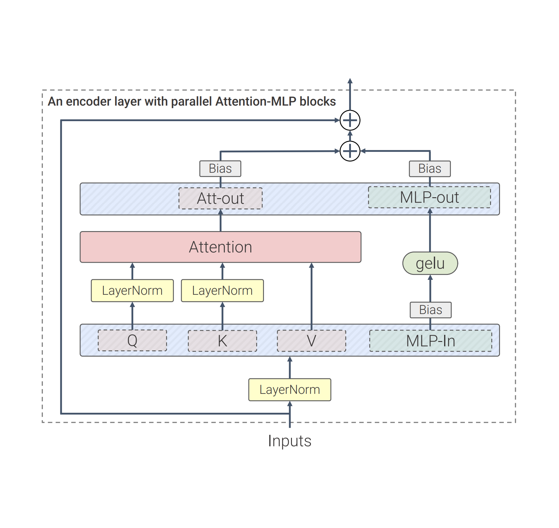
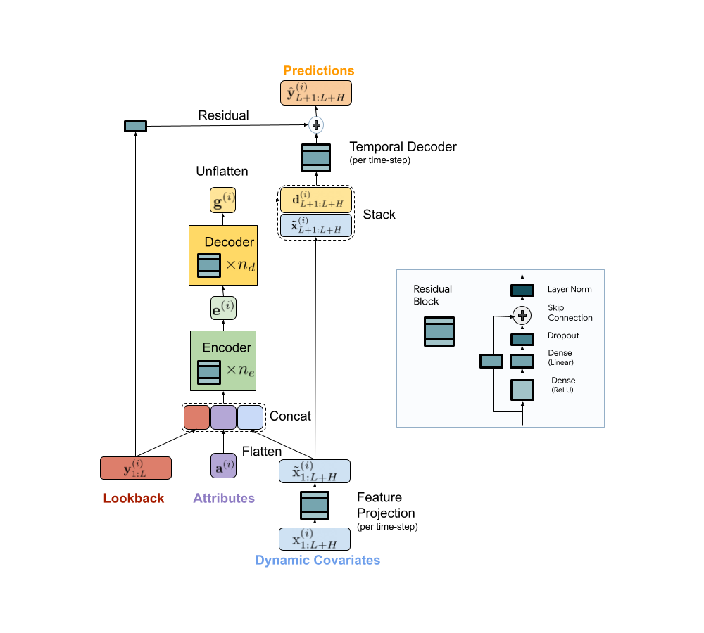
We present a scalable MLP-based encoder-decoder model for fast and accurate multi-step forecasting. Our model encodes the past of a time-series and all available features using an MLP encoder. Subsequently, the encoding is combined with future features using an MLP decoder to yield future predictions. The architecture is illustrated below.

TiDE model architecture for multi-step forecasting.

TiDE is more than 10x faster in training compared to transformer-based baselines while being more accurate on benchmarks. Similar gains can be observed in inference as it only scales linearly with the length of the context (the number of time-steps the model looks back) and the prediction horizon. Below on the left, we show that our model can be 10.6% better than the best transformer-based baseline (PatchTST) on a popular traffic forecasting benchmark, in terms of test mean squared error (MSE). On the right, we show that at the same time our model can have much faster inference latency than PatchTST.

Left: MSE on the test set of a popular traffic forecasting benchmark. Right: inference time of TiDE and PatchTST as a function of the look-back length.

Our research demonstrates that we can take advantage of MLP’s linear computational scaling with look-back and horizon sizes without sacrificing accuracy, while transformers scale quadratically in this situation.


Probabilistic loss functions

In most forecasting applications the end user is interested in popular target metrics like the mean absolute percentage error (MAPE), weighted absolute percentage error (WAPE), etc. In such scenarios, the standard approach is to use the same target metric as the loss function while training. In “On the benefits of maximum likelihood estimation for Regression and Forecasting”, accepted at ICLR, we show that this approach might not always be the best. Instead, we advocate using the maximum likelihood loss for a carefully chosen family of distributions (discussed more below) that can capture inductive biases of the dataset during training. In other words, instead of directly outputting point predictions that minimize the target metric, the forecasting neural network predicts the parameters of a distribution in the chosen family that best explains the target data. At inference time, we can predict the statistic from the learned predictive distribution that minimizes the target metric of interest (e.g., the mean minimizes the MSE target metric while the median minimizes the WAPE). Further, we can also easily obtain uncertainty estimates of our forecasts, i.e., we can provide quantile forecasts by estimating the quantiles of the predictive distribution. In several use cases, accurate quantiles are vital, for instance, in demand forecasting a retailer might want to stock for the 90th percentile to guard against worst-case scenarios and avoid lost revenue.

The choice of the distribution family is crucial in such cases. For example, in the context of sparse count data, we might want to have a distribution family that can put more probability on zero, which is commonly known as zero-inflation. We propose a mixture of different distributions with learned mixture weights that can adapt to different data modalities. In the paper, we show that using a mixture of zero and multiple negative binomial distributions works well in a variety of settings as it can adapt to sparsity, multiple modalities, count data, and data with sub-exponential tails.

A mixture of zero and two negative binomial distributions. The weights of the three components, a1, a2 and a3, can be learned during training.

We use this loss function for training Vertex AutoML models on the M5 forecasting competition dataset and show that this simple change can lead to a 6% gain and outperform other benchmarks in the competition metric, weighted root mean squared scaled error (WRMSSE).


M5 Forecasting WRMSSE
Vertex AutoML 0.639 +/- 0.007
Vertex AutoML with probabilistic loss       0.581 +/- 0.007
DeepAR 0.789 +/- 0.025
FEDFormer 0.804 +/- 0.033

Conclusion

We have shown how TiDE, together with probabilistic loss functions, enables fast and accurate forecasting that automatically adapts to different data distributions and modalities and also provides uncertainty estimates for its predictions. It provides state-of-the-art accuracy among neural network–based solutions at a fraction of the cost of previous transformer-based forecasting architectures, for large-scale enterprise forecasting applications. We hope this work will also spur interest in revisiting (both theoretically and empirically) MLP-based deep time-series forecasting models.


Acknowledgements

This work is the result of a collaboration between several individuals across Google Research and Google Cloud, including (in alphabetical order): Pranjal Awasthi, Dawei Jia, Weihao Kong, Andrew Leach, Shaan Mathur, Petros Mol, Shuxin Nie, Ananda Theertha Suresh, and Rose Yu.

Source: Google AI Blog


Differentially private heatmaps

Recently, differential privacy (DP) has emerged as a mathematically robust notion of user privacy for data aggregation and machine learning (ML), with practical deployments including the 2022 US Census and in industry. Over the last few years, we have open-sourced libraries for privacy-preserving analytics and ML and have been constantly enhancing their capabilities. Meanwhile, new algorithms have been developed by the research community for several analytic tasks involving private aggregation of data.

One such important data aggregation method is the heatmap. Heatmaps are popular for visualizing aggregated data in two or more dimensions. They are widely used in many fields including computer vision, image processing, spatial data analysis, bioinformatics, and more. Protecting the privacy of user data is critical for many applications of heatmaps. For example, heatmaps for gene microdata are based on private data from individuals. Similarly, a heatmap of popular locations in a geographic area are based on user location check-ins that need to be kept private.

Motivated by such applications, in “Differentially Private Heatmaps” (presented at AAAI 2023), we describe an efficient DP algorithm for computing heatmaps with provable guarantees and evaluate it empirically. At the core of our DP algorithm for heatmaps is a solution to the basic problem of how to privately aggregate sparse input vectors (i.e., input vectors with a small number of non-zero coordinates) with a small error as measured by the Earth Mover's Distance (EMD). Using a hierarchical partitioning procedure, our algorithm views each input vector, as well as the output heatmap, as a probability distribution over a number of items equal to the dimension of the data. For the problem of sparse aggregation under EMD, we give an efficient algorithm with error asymptotically close to the best possible.


Algorithm description

Our algorithm works by privatizing the aggregated distribution (obtained by averaging over all user inputs), which is sufficient for computing a final heatmap that is private due to the post-processing property of DP. This property ensures that any transformation of the output of a DP algorithm remains differentially private. Our main contribution is a new privatization algorithm for the aggregated distribution, which we will describe next.

The EMD measure, which is a distance-like measure of dissimilarity between two probability distributions originally proposed for computer vision tasks, is well-suited for heatmaps since it takes the underlying metric space into account and considers "neighboring" bins. EMD is used in a variety of applications including deep learning, spatial analysis, human mobility, image retrieval, face recognition, visual tracking, shape matching, and more.

To achieve DP, we need to add noise to the aggregated distribution. We would also like to preserve statistics at different scales of the grid to minimize the EMD error. So, we create a hierarchical partitioning of the grid, add noise at each level, and then recombine into the final DP aggregated distribution. In particular, the algorithm has the following steps:

  1. Quadtree construction: Our hierarchical partitioning procedure first divides the grid into four cells, then divides each cell into four subcells; it recursively continues this process until each cell is a single pixel. This procedure creates a quadtree over the subcells where the root represents the entire grid and each leaf represents a pixel. The algorithm then calculates the total probability mass for each tree node (obtained by adding up the aggregated distribution’s probabilities of all leaves in the subtree rooted at this node). This step is illustrated below.
    In the first step, we take the (non-private) aggregated distribution (top left) and repeatedly divide it to create a quadtree. Then, we compute the total probability mass is each cell (bottom).
  2. Noise addition: To each tree node’s mass we then add Laplace noise calibrated to the use case.
  3. Truncation: To help reduce the final amount of noise in our DP aggregated distribution, the algorithm traverses the tree starting from the root and, at each level, it discards all but the top w nodes with highest (noisy) masses together with their descendants.
  4. Reconstruction: Finally, the algorithm solves a linear program to recover the aggregated distribution. This linear program is inspired by the sparse recovery literature where the noisy masses are viewed as (noisy) measurements of the data.
In step 2, noise is added to each cell’s probability mass. Then in step 3, only top-w cells are kept (green) whereas the remaining cells are truncated (red). Finally, in the last step, we write a linear program on these top cells to reconstruct the aggregation distribution, which is now differentially private.

Experimental results

We evaluate the performance of our algorithm in two different domains: real-world location check-in data and image saliency data. We consider as a baseline the ubiquitous Laplace mechanism, where we add Laplace noise to each cell, zero out any negative cells, and produce the heatmap from this noisy aggregate. We also consider a “thresholding” variant of this baseline that is more suited to sparse data: only keep top t% of the cell values (based on the probability mass in each cell) after noising while zeroing out the rest. To evaluate the quality of an output heatmap compared to the true heatmap, we use Pearson coefficient, KL-divergence, and EMD. Note that when the heatmaps are more similar, the first metric increases but the latter two decrease.

The locations dataset is obtained by combining two datasets, Gowalla and Brightkite, both of which contain check-ins by users of location-based social networks. We pre-processed this dataset to consider only check-ins in the continental US resulting in a final dataset consisting of ~500,000 check-ins by ~20,000 users. Considering the top cells (from an initial partitioning of the entire space into a 300 x 300 grid) that have check-ins from at least 200 unique users, we partition each such cell into subgrids with a resolution of ∆ × ∆ and assign each check-in to one of these subgrids.

In the first set of experiments, we fix ∆ = 256. We test the performance of our algorithm for different values of ε (the privacy parameter, where smaller ε means stronger DP guarantees), ranging from 0.1 to 10, by running our algorithms together with the baseline and its variants on all cells, randomly sampling a set of 200 users in each trial, and then computing the distance metrics between the true heatmap and the DP heatmap. The average of these metrics is presented below. Our algorithm (the red line) performs better than all versions of the baseline across all metrics, with improvements that are especially significant when ε is not too large or small (i.e., 0.2 ≤ ε ≤ 5).

Metrics averaged over 60 runs when varying ε for the location dataset. Shaded areas indicate 95% confidence interval.

Next, we study the effect of varying the number n of users. By fixing a single cell (with > 500 users) and ε, we vary n from 50 to 500 users. As predicted by theory, our algorithms and the baseline perform better as n increases. However, the behavior of the thresholding variants of the baseline are less predictable.

We also run another experiment where we fix a single cell and ε, and vary the resolution ∆ from 64 to 256. In agreement with theory, our algorithm’s performance remains nearly constant for the entire range of ∆. However, the baseline suffers across all metrics as ∆ increases while the thresholding variants occasionally improve as ∆ increases.

Effect of the number of users and grid resolution on EMD.

We also experiment on the Salicon image saliency dataset (SALICON). This dataset is a collection of saliency annotations on the Microsoft Common Objects in Context image database. We downsized the images to a fixed resolution of 320 × 240 and each [user, image] pair consists of a sequence of coordinates in the image where the user looked. We repeat the experiments described previously on 38 randomly sampled images (with ≥ 50 users each) from SALICON. As we can see from the examples below, the heatmap obtained by our algorithm is very close to the ground truth.

Example visualization of different algorithms for two different natural images from SALICON for ε = 10 and n = 50 users. The algorithms from left to right are: original heatmap (no privacy), baseline, and ours.

Additional experimental results, including those on other datasets, metrics, privacy parameters and DP models, can be found in the paper.


Conclusion

We presented a privatization algorithm for sparse distribution aggregation under the EMD metric, which in turn yields an algorithm for producing privacy-preserving heatmaps. Our algorithm extends naturally to distributed models that can implement the Laplace mechanism, including the secure aggregation model and the shuffle model. This does not apply to the more stringent local DP model, and it remains an interesting open question to devise practical local DP heatmap/EMD aggregation algorithms for “moderate” number of users and privacy parameters.


Acknowledgments

This work was done jointly with Junfeng He, Kai Kohlhoff, Ravi Kumar, Pasin Manurangsi, and Vidhya Navalpakkam.

Source: Google AI Blog


Beyond automatic differentiation

Derivatives play a central role in optimization and machine learning. By locally approximating a training loss, derivatives guide an optimizer toward lower values of the loss. Automatic differentiation frameworks such as TensorFlow, PyTorch, and JAX are an essential part of modern machine learning, making it feasible to use gradient-based optimizers to train very complex models.

But are derivatives all we need? By themselves, derivatives only tell us how a function behaves on an infinitesimal scale. To use derivatives effectively, we often need to know more than that. For example, to choose a learning rate for gradient descent, we need to know something about how the loss function behaves over a small but finite window. A finite-scale analogue of automatic differentiation, if it existed, could help us make such choices more effectively and thereby speed up training.

In our new paper "Automatically Bounding The Taylor Remainder Series: Tighter Bounds and New Applications", we present an algorithm called AutoBound that computes polynomial upper and lower bounds on a given function, which are valid over a user-specified interval. We then begin to explore AutoBound's applications. Notably, we present a meta-optimizer called SafeRate that uses the upper bounds computed by AutoBound to derive learning rates that are guaranteed to monotonically reduce a given loss function, without the need for time-consuming hyperparameter tuning. We are also making AutoBound available as an open-source library.


The AutoBound algorithm

Given a function f and a reference point x0, AutoBound computes polynomial upper and lower bounds on f that hold over a user-specified interval called a trust region. Like Taylor polynomials, the bounding polynomials are equal to f at x0. The bounds become tighter as the trust region shrinks, and approach the corresponding Taylor polynomial as the trust region width approaches zero.

Automatically-derived quadratic upper and lower bounds on a one-dimensional function f, centered at x0=0.5. The upper and lower bounds are valid over a user-specified trust region, and become tighter as the trust region shrinks.

Like automatic differentiation, AutoBound can be applied to any function that can be implemented using standard mathematical operations. In fact, AutoBound is a generalization of Taylor mode automatic differentiation, and is equivalent to it in the special case where the trust region has a width of zero.

To derive the AutoBound algorithm, there were two main challenges we had to address:

  1. We had to derive polynomial upper and lower bounds for various elementary functions, given an arbitrary reference point and arbitrary trust region.
  2. We had to come up with an analogue of the chain rule for combining these bounds.

Bounds for elementary functions

For a variety of commonly-used functions, we derive optimal polynomial upper and lower bounds in closed form. In this context, "optimal" means the bounds are as tight as possible, among all polynomials where only the maximum-degree coefficient differs from the Taylor series. Our theory applies to elementary functions, such as exp and log, and common neural network activation functions, such as ReLU and Swish. It builds upon and generalizes earlier work that applied only to quadratic bounds, and only for an unbounded trust region.

Optimal quadratic upper and lower bounds on the exponential function, centered at x0=0.5 and valid over the interval [0, 2].

A new chain rule

To compute upper and lower bounds for arbitrary functions, we derived a generalization of the chain rule that operates on polynomial bounds. To illustrate the idea, suppose we have a function that can be written as

f(x) = g(h(x))

and suppose we already have polynomial upper and lower bounds on g and h. How do we compute bounds on f?

The key turns out to be representing the upper and lower bounds for a given function as a single polynomial whose highest-degree coefficient is an interval rather than a scalar. We can then plug the bound for h into the bound for g, and convert the result back to a polynomial of the same form using interval arithmetic. Under suitable assumptions about the trust region over which the bound on g holds, it can be shown that this procedure yields the desired bound on f.

The interval polynomial chain rule applied to the functions h(x) = sqrt(x) and g(y) = exp(y), with x0=0.25 and trust region [0, 0.5].

Our chain rule applies to one-dimensional functions, but also to multivariate functions, such as matrix multiplications and convolutions.


Propagating bounds

Using our new chain rule, AutoBound propagates interval polynomial bounds through a computation graph from the inputs to the outputs, analogous to forward-mode automatic differentiation.

Forward propagation of interval polynomial bounds for the function f(x) = exp(sqrt(x)). We first compute (trivial) bounds on x, then use the chain rule to compute bounds on sqrt(x) and exp(sqrt(x)).

To compute bounds on a function f(x), AutoBound requires memory proportional to the dimension of x. For this reason, practical applications apply AutoBound to functions with a small number of inputs. However, as we will see, this does not prevent us from using AutoBound for neural network optimization.


Automatically deriving optimizers, and other applications

What can we do with AutoBound that we couldn't do with automatic differentiation alone?

Among other things, AutoBound can be used to automatically derive problem-specific, hyperparameter-free optimizers that converge from any starting point. These optimizers iteratively reduce a loss by first using AutoBound to compute an upper bound on the loss that is tight at the current point, and then minimizing the upper bound to obtain the next point.

Minimizing a one-dimensional logistic regression loss using quadratic upper bounds derived automatically by AutoBound.

Optimizers that use upper bounds in this way are called majorization-minimization (MM) optimizers. Applied to one-dimensional logistic regression, AutoBound rederives an MM optimizer first published in 2009. Applied to more complex problems, AutoBound derives novel MM optimizers that would be difficult to derive by hand.

We can use a similar idea to take an existing optimizer such as Adam and convert it to a hyperparameter-free optimizer that is guaranteed to monotonically reduce the loss (in the full-batch setting). The resulting optimizer uses the same update direction as the original optimizer, but modifies the learning rate by minimizing a one-dimensional quadratic upper bound derived by AutoBound. We refer to the resulting meta-optimizer as SafeRate.

Performance of SafeRate when used to train a single-hidden-layer neural network on a subset of the MNIST dataset, in the full-batch setting.

Using SafeRate, we can create more robust variants of existing optimizers, at the cost of a single additional forward pass that increases the wall time for each step by a small factor (about 2x in the example above).

In addition to the applications just discussed, AutoBound can be used for verified numerical integration and to automatically prove sharper versions of Jensen's inequality, a fundamental mathematical inequality used frequently in statistics and other fields.


Improvement over classical bounds

Bounding the Taylor remainder term automatically is not a new idea. A classical technique produces degree k polynomial bounds on a function f that are valid over a trust region [a, b] by first computing an expression for the kth derivative of f (using automatic differentiation), then evaluating this expression over [a,b] using interval arithmetic.

While elegant, this approach has some inherent limitations that can lead to very loose bounds, as illustrated by the dotted blue lines in the figure below.

Quadratic upper and lower bounds on the loss of a multi-layer perceptron with two hidden layers, as a function of the initial learning rate. The bounds derived by AutoBound are much tighter than those obtained using interval arithmetic evaluation of the second derivative.

Looking forward

Taylor polynomials have been in use for over three hundred years, and are omnipresent in numerical optimization and scientific computing. Nevertheless, Taylor polynomials have significant limitations, which can limit the capabilities of algorithms built on top of them. Our work is part of a growing literature that recognizes these limitations and seeks to develop a new foundation upon which more robust algorithms can be built.

Our experiments so far have only scratched the surface of what is possible using AutoBound, and we believe it has many applications we have not discovered. To encourage the research community to explore such possibilities, we have made AutoBound available as an open-source library built on top of JAX. To get started, visit our GitHub repo.


Acknowledgements

This post is based on joint work with Josh Dillon. We thank Alex Alemi and Sergey Ioffe for valuable feedback on an earlier draft of the post.

Source: Google AI Blog


Google Dev Library Newsletter: 20th Edition

Posted by the Dev Library team

In this newsletter, we’re highlighting the best projects developed with Google technologies that have been contributed to the Google Dev Library platform. We hope this will spark some inspiration for your next project!


Highlights of the Month - Cloud Champions


Google Anthos in a nutshell by Navveen Balani


GCP Anthos Config Management Architecture

Dive into the overview on Anthos Service Mesh (ASM) and go through the topology supported by ASM and high level steps to implement multi cluster service mesh on a single and multiple VPC network.

Read more on Dev Library


Google Cloud Contact Center Artificial Intelligence (CCAI) by Rubens Zimbres

Explore the concept of CCAI and how it can be used to improve customer service, along with tools that can be integrated with existing contact center infrastructure to automate and optimize various processes.

Read more on Dev Library


Build a chat server with Cloud Run by Jaeyeon Baek

Explore how to build a chat server with Cloud Run using Python as the development language with the FastAPI framework.

Read more on Dev Library


Android


DocuBox by Vaibhav Jaiswal

Learn to build an app like DocuBox, which is designed to manage and organize documents on an Android device.

WebRTC Android by Jaewoong Eum

Understand how the WebRTC pre-compiled library for Android reflects the recent WebRTC updates to facilitate real-time video chat for Android.

WebRTC in Jetpack Compose by Jaewoong Eum

Discover how the project demonstrates WebRTC protocol to facilitate real-time video communications with Jetpack Compose.

TabSync, a lightweight synchronizer between Android's Tabs and Lists by Ahmad Hamwi

Learn how to add a synchronizer between Android’s RecyclerView and TabLayout, and what are the use cases of such on mobile devices.


Angular


Directives in practice: user role-based element control by Paweł Kubiak

Explore the concept of structural and attribute directives in Angular, which can be added to HTML elements to modify behavior or appearance.


Flutter


Ultimate guide to becoming a Flutter expert by Isaac Adariku

Become an Expert Flutter developer by mastering these concepts.

Handling complex HTML in Flutter by Tanmoy Karmakar

Discover how to handle complex HTML content like tables, images, and links in a Flutter app using the flutter_html package.

Firebase Cloud Messaging (FCM) with Flutter by Ayesha Iftikhar

Learn how to use FCM in Flutter apps. FCM is a cloud messaging service that allows you to send notifications and messages to devices on different platforms, including Android, iOS, and the web.

Understanding app localization in Flutter by Caleb Jesusegun

Take a deep dive into app localization and learn how to implement it in Flutter using the intl package.


Machine Learning


Visualizing custom TFX artifacts with InteractiveContext by Suzen Fylke

Learn how you can use InteractiveContext to visualize custom TFX artifacts.

How is generative machine learning transforming finance? By Hannes Hapke

Follow these detailed steps to adopt large generative models for domain-specific, fine-tuned generative models using the TensorFlow ecosystem.


Directing ML toward natural hazard mitigation through collaboration

Floods are the most common type of natural disaster, affecting more than 250 million people globally each year. As part of Google's Crisis Response and our efforts to address the climate crisis, we are using machine learning (ML) models for Flood Forecasting to alert people in areas that are impacted before disaster strikes.

Collaboration between researchers in the industry and academia is essential for accelerating progress towards mutual goals in ML-related research. Indeed, Google's current ML-based flood forecasting approach was developed in collaboration with researchers (1, 2) at the Johannes Kepler University in Vienna, Austria, the University of Alabama, and the Hebrew University of Jerusalem, among others.

Today we discuss our recent Machine Learning Meets Flood Forecasting Workshop, which highlights efforts to bring together researchers from Google and other universities and organizations to advance our understanding of flood behavior and prediction, and build more robust solutions for early detection and warning. We also discuss the Caravan project, which is helping to create an open-source repository for global streamflow data, and is itself an example of a collaboration that developed from the previous Flood Forecasting Meets Machine Learning Workshop.


2023 Machine Learning Meets Flood Forecasting Workshop

The fourth annual Google Machine Learning Meets Flood Forecasting Workshop was held in January. This 2-day virtual workshop hosted over 100 participants from 32 universities, 20 governmental and non-governmental agencies, and 11 private companies. This forum provided an opportunity for hydrologists, computer scientists, and aid workers to discuss challenges and efforts toward improving global flood forecasts, to keep up with state-of-the-art technology advances, and to integrate domain knowledge into ML-based forecasting approaches.

The event included talks from six invited speakers, a series of small-group discussion sessions focused on hydrological modeling, inundation mapping, and hazard alerting–related topics, as well as a presentation by Google on the FloodHub, which provides free, public access to Google’s flood forecasts, up to 7 days in advance.

Invited speakers at the workshop included:

The presentations can be viewed on YouTube:

2023 Flood Forecasting Meets Machine Learning Talks Day 1


2023 Flood Forecasting Meets Machine Learning Talks Day 2


Some of the top challenges highlighted during the workshop were related to the integration of physical and hydrological science with ML to help build trust and reliability; filling gaps in observations of inundated areas with models and satellite data; measuring the skill and reliability of flood warning systems; and improving the communication of flood warnings to diverse, global populations. In addition, participants stressed that addressing these and other challenges will require collaboration between a number of different organizations and scientific disciplines.


The Caravan project

One of the main challenges in conducting successful ML research and creating advanced tools for flood forecasting is the need for large amounts of data for computationally expensive training and evaluation. Today, many countries and organizations collect streamflow data (typically either water levels or flow rates), but it is not standardized or held in a central repository, which makes it difficult for researchers to access.

During the 2019 Machine Learning Meets Flood Forecasting Workshop, a group of researchers identified the need for an open source, global streamflow data repository, and developed ideas around leveraging free computational resources from Google Earth Engine to address the flood forecasting community’s challenge of data collection and accessibility. Following two years of collaborative work between researchers from Google, the school of Geography at the University of Exeter, the Institute for Machine Learning at Johannes Kepler University, and the Institute for Atmospheric and Climate Science at ETH Zurich, the Caravan project was created.

In “Caravan - A global community dataset for large-sample hydrology”, published in Nature Scientific Data, we describe the project in more detail. Based on a global dataset for the development and training of hydrological models (see figure below), Caravan provides open-source Python scripts that leverage essential weather and geographical data that was previously made public on Google Earth Engine to match streamflow data that users upload to the repository. This repository originally contained data from more than 13,000 watersheds in Central Europe, Brazil, Chile, Australia, the United States, Canada, and Mexico. It has further benefited from community contributions from the Geological Survey of Denmark and Greenland that includes streamflow data from most of the watersheds in Denmark. The goal is to continue to develop and grow this repository to enable researchers to access most of the world’s streamflow data. For more information regarding contributing to the Caravan dataset, reach out to [email protected].

Locations of the 13,000 streamflow gauges in the Caravan dataset and the distribution of those gauges in GEnS global climate zones.

The path forward

Google plans to continue to host these workshops to help broaden and deepen collaboration between industry and academia in the development of environmental AI models. We are looking forward to seeing what advances might come out of the most recent workshop. Hydrologists and researchers interested in participating in future workshops are encouraged to contact [email protected].

Source: Google AI Blog


Scaling vision transformers to 22 billion parameters

Large Language Models (LLMs) like PaLM or GPT-3 showed that scaling transformers to hundreds of billions of parameters improves performance and unlocks emergent abilities. The biggest dense models for image understanding, however, have reached only 4 billion parameters, despite research indicating that promising multimodal models like PaLI continue to benefit from scaling vision models alongside their language counterparts. Motivated by this, and the results from scaling LLMs, we decided to undertake the next step in the journey of scaling the Vision Transformer.

In “Scaling Vision Transformers to 22 Billion Parameters”, we introduce the biggest dense vision model, ViT-22B. It is 5.5x larger than the previous largest vision backbone, ViT-e, which has 4 billion parameters. To enable this scaling, ViT-22B incorporates ideas from scaling text models like PaLM, with improvements to both training stability (using QK normalization) and training efficiency (with a novel approach called asynchronous parallel linear operations). As a result of its modified architecture, efficient sharding recipe, and bespoke implementation, it was able to be trained on Cloud TPUs with a high hardware utilization1. ViT-22B advances the state of the art on many vision tasks using frozen representations, or with full fine-tuning. Further, the model has also been successfully used in PaLM-e, which showed that a large model combining ViT-22B with a language model can significantly advance the state of the art in robotics tasks.


Architecture

Our work builds on many advances from LLMs, such as PaLM and GPT-3. Compared to the standard Vision Transformer architecture, we use parallel layers, an approach in which attention and MLP blocks are executed in parallel, instead of sequentially as in the standard Transformer. This approach was used in PaLM and reduced training time by 15%.

Secondly, ViT-22B omits biases in the QKV projections, part of the self-attention mechanism, and in the LayerNorms, which increases utilization by 3%. The diagram below shows the modified transformer architecture used in ViT-22B:

ViT-22B transformer encoder architecture uses parallel feed-forward layers, omits biases in QKV and LayerNorm layers and normalizes Query and Key projections.

Models at this scale necessitate “sharding” — distributing the model parameters in different compute devices. Alongside this, we also shard the activations (the intermediate representations of an input). Even something as simple as a matrix multiplication necessitates extra care, as both the input and the matrix itself are distributed across devices. We develop an approach called asynchronous parallel linear operations, whereby communications of activations and weights between devices occur at the same time as computations in the matrix multiply unit (the part of the TPU holding the vast majority of the computational capacity). This asynchronous approach minimizes the time waiting on incoming communication, thus increasing device efficiency. The animation below shows an example computation and communication pattern for a matrix multiplication.

Asynchronized parallel linear operation. The goal is to compute the matrix multiplication y = Ax, but both the matrix A and activation x are distributed across different devices. Here we illustrate how it can be done with overlapping communication and computation across devices. The matrix A is column-sharded across the devices, each holding a contiguous slice, each block represented as Aij. More details are in the paper.

At first, the new model scale resulted in severe training instabilities. The normalization approach of Gilmer et al. (2023, upcoming) resolved these issues, enabling smooth and stable model training; this is illustrated below with example training progressions.

The effect of normalizing the queries and keys (QK normalization) in the self-attention layer on the training dynamics. Without QK normalization (red) gradients become unstable and the training loss diverges.

Results

Here we highlight some results of ViT-22B. Note that in the paper we also explore several other problem domains, like video classification, depth estimation, and semantic segmentation.

To illustrate the richness of the learned representation, we train a text model to produce representations that align text and image representations (using LiT-tuning). Below we show several results for out-of-distribution images generated by Parti and Imagen:

Examples of image+text understanding for ViT-22B paired with a text model. The graph shows normalized probability distribution for each description of an image.

Human object recognition alignment

To find out how aligned ViT-22B classification decisions are with human classification decisions, we evaluated ViT-22B fine-tuned with different resolutions on out-of-distribution (OOD) datasets for which human comparison data is available via the model-vs-human toolbox. This toolbox measures three key metrics: How well do models cope with distortions (accuracy)? How different are human and model accuracies (accuracy difference)? Finally, how similar are human and model error patterns (error consistency)? While not all fine-tuning resolutions perform equally well, ViT-22B variants are state of the art for all three metrics. Furthermore, the ViT-22B models also have the highest ever recorded shape bias in vision models. This means that they mostly use object shape, rather than object texture, to inform classification decisions — a strategy known from human perception (which has a shape bias of 96%). Standard models (e.g., ResNet-50, which has aa ~20–30% shape bias) often classify images like the cat with elephant texture below according to the texture (elephant); models with a high shape bias tend to focus on the shape instead (cat). While there are still many important differences between human and model perception, ViT-22B shows increased similarities to human visual object recognition.

Cat or elephant? Car or clock? Bird or bicycle? Example images with the shape of one object and the texture of a different object, used to measure shape/texture bias.
Shape bias evaluation (higher = more shape-biased). Many vision models have a low shape / high texture bias, whereas ViT-22B fine-tuned on ImageNet (red, green, blue trained on 4B images as indicated by brackets after model names, unless trained on ImageNet only) have the highest shape bias recorded in a ML model to date, bringing them closer to a human-like shape bias.

Out-of-distribution performance

Measuring performance on OOD datasets helps assess generalization. In this experiment we construct label-maps (mappings of labels between datasets) from JFT to ImageNet and also from ImageNet to different out-of-distribution datasets like ObjectNet (results after pre-training on this data shown in the left curve below). Then the models are fully fine-tuned on ImageNet.

We observe that scaling Vision Transformers increases OOD performance: even though ImageNet accuracy saturates, we see a significant increase on ObjectNet from ViT-e to ViT-22B (shown by the three orange dots in the upper right below).

Even though ImageNet accuracy saturates, we see a significant increase in performance on ObjectNet from ViT-e/14 to ViT-22B.

Linear probe

Linear probe is a technique where a single linear layer is trained on top of a frozen model. Compared to full fine-tuning, this is much cheaper to train and easier to set up. We observed that the linear probe of ViT-22B performance approaches that of state-of-the-art full fine-tuning of smaller models using high-resolution images (training with higher resolution is generally much more expensive, but for many tasks it yields better results). Here are results of a linear probe trained on the ImageNet dataset and evaluated on the ImageNet validation dataset and other OOD ImageNet datasets.

Linear probe results trained on ImageNet, evaluated on Imagenet-ReaL, ImageNet-v2, ObjectNet, ImageNet-R and ImageNet-A datasets. High-resolution fine-tuned ViT-e/14 provided as a reference.

Distillation

The knowledge of the bigger model can be transferred to a smaller model using the distillation method. This is helpful as big models are slower and more expensive to use. We found that ViT-22B knowledge can be transferred to smaller models like ViT-B/16 and ViT-L/16, achieving a new state of the art on ImageNet for those model sizes.


Model Approach (dataset) ImageNet1k Accuracy
ViT-B/16       Transformers for Image Recognition at Scale (JFT)       84.2
Scaling Vision Transformers (JFT) 86.6
DeiT III: Revenge of the ViT (INet21k) 86.7
Distilled from ViT-22B (JFT) 88.6
   
ViT-L/16 Transformers for Image Recognition at Scale (JFT) 87.1
Scaling Vision Transformers (JFT) 88.5
DeiT III: Revenge of the ViT (INet21k) 87.7
Distilled from ViT-22B (JFT) 89.6


Fairness and bias

ML models can be susceptible to unintended unfair biases, such as picking up spurious correlations (measured using demographic parity) or having performance gaps across subgroups. We show that scaling up the size helps in mitigating such issues.

First, scale offers a more favorable tradeoff frontier — performance improves with scale even when the model is post-processed after training to control its level of demographic parity below a prescribed, tolerable level. Importantly, this holds not only when performance is measured in terms of accuracy, but also other metrics, such as calibration, which is a statistical measure of the truthfulness of the model's estimated probabilities. Second, classification of all subgroups tends to improve with scale as demonstrated below. Third, ViT-22B reduces the performance gap across subgroups.


Top: Accuracy for each subgroup in CelebA before debiasing. Bottom: The y-axis shows the absolute difference in performance across the two specific subgroups highlighted in this example: females and males. ViT-22B has a small gap in performance compared to smaller ViT architectures.

Conclusions

We have presented ViT-22B, currently the largest vision transformer model at 22 billion parameters. With small but critical changes to the original architecture, we achieved excellent hardware utilization and training stability, yielding a model that advances the state of the art on several benchmarks. Great performance can be achieved using the frozen model to produce embeddings and then training thin layers on top. Our evaluations further show that ViT-22B shows increased similarities to human visual perception when it comes to shape and texture bias, and offers benefits in fairness and robustness, when compared to existing models.


Acknowledgements

This is a joint work of Mostafa Dehghani, Josip Djolonga, Basil Mustafa, Piotr Padlewski, Jonathan Heek, Justin Gilmer, Andreas Steiner, Mathilde Caron, Robert Geirhos, Ibrahim Alabdulmohsin, Rodolphe Jenatton, Lucas Beyer, Michael Tschannen, Anurag Arnab, Xiao Wang, Carlos Riquelme, Matthias Minderer, Joan Puigcerver, Utku Evci, Manoj Kumar, Sjoerd van Steenkiste, Gamaleldin Fathy, Elsayed Aravindh Mahendran, Fisher Yu, Avital Oliver, Fantine Huot, Jasmijn Bastings, Mark Patrick Collier, Alexey Gritsenko, Vighnesh Birodkar, Cristina Vasconcelos, Yi Tay, Thomas Mensink, Alexander Kolesnikov, Filip Pavetić, Dustin Tran, Thomas Kipf, Mario Lučić, Xiaohua Zhai, Daniel Keysers Jeremiah Harmsen, and Neil Houlsby

We would like to thank Jasper Uijlings, Jeremy Cohen, Arushi Goel, Radu Soricut, Xingyi Zhou, Lluis Castrejon, Adam Paszke, Joelle Barral, Federico Lebron, Blake Hechtman, and Peter Hawkins. Their expertise and unwavering support played a crucial role in the completion of this paper. We also acknowledge the collaboration and dedication of the talented researchers and engineers at Google Research.


1Note: ViT-22B has 54.9% model FLOPs utilization (MFU) while PaLM reported 46.2% MFU and we measured 44.0% MFU for ViT-e on the same hardware. 

Source: Google AI Blog


GDE Women’s History Month Feature: Jigyasa Grover, Machine Learning

Posted by Kevin Hernandez, Developer Relations Community Manager

For Women’s History Month, we are celebrating Jigyasa Grover, ML GDE.

Photo of Jigyasa Grover, holding a cup of coffee, smiling
Jigyasa Grover, ML GDE, Senior ML Engineer, Twitter

Jigyasa Grover is a 10x award winner in AI and open source, a published book author in machine learning, and was most recently named one of the 50 most powerful women in technology to follow for 2023. Jigyasa has always been inspired by technology – with her father being a computer scientist for the government of India and playing with a toy laptop as a child. Google has also played an integral role in her career by providing resources and community every step of the way: from early in her university days through Google Summer of Code to today, where she is a Senior ML Engineer at Twitter and leverages the Women Techmakers and Google Developer Experts programs to connect with other developers and pay it forward through programs like Google Code-In.

Getting involved in the developer community

Things started rolling for Jigyasa in her first year at university when she discovered Pharo at the library, where she spent a lot of her time. As she started to dive deeper into Pharo, she read more and more about the open source community and eventually started reaching out to members of the community online. This led her to discover Google Summer of Code, an open source internship, where she was selected to participate as one of the youngest developers. After a successful stint in the program, Jigyasa was invited to participate again the following year, which proved to be a pivotal moment in her academic career. Up to this point, Jigyasa was working primarily on mobile and web app development. “The second year, the project that I was working on was more focused on building web scrapers, machine learning, NLP chatbots, and so on. That was my introduction to the world of machine learning which got me intrigued”, Jigyasa says. After this experience she started taking more courses related to machine learning, watched talks, worked on more machine learning projects, and interned at the National Research Council of Canada and then the Institute Research and Development in France. These experiences helped shape her career vision and she knew that machine learning would be her field of expertise.

Finding community through Google

Up until college, Jigyasa had always gone to all-girls schools so when she first got to engineering school, it was an eye-opening experience for her. She reflects, “I felt like a minority coming from a place where I was surrounded by girls all the time. That's when I started Googling different organizations and found organizations like Women Who Code, Women Techmakers, and Google Developer Groups.” These organizations exposed her to mentorship, resources, and events, and more. One such event was Google I/O, where she was invited to attend online. Many developer events reminded her of the lack of women's representation in the developer community. This inspired her to commit to the saying, "be the change you want to see in the world." Jigyasa would go on to pursue speaking opportunities at tech events and inspire other women developers with her passion and support.

After university, Jigyasa discovered the GDE program and the strong community the program offers. Jigyasa adds, “I think one of the most meaningful parts of the program is the community. I like how different Google programs cater to different kinds of audiences. For example, when I became a GDE, I was a part of the wider developer community but also connected with developers in my field of expertise - machine learning.” Jigyasa appreciates being able to interact with people in her field and is motivated by being surrounded by like-minded people. She has even been a guest on another GDE’s YouTube channel and was also given a chance to connect with Laurence Moroney, Lead AI Advocate at Google, who wrote the foreword for her book. Jigyasa credits Google developer programs for developing her career and expertise, “All of these programs have brought me great opportunities. Summer of Code, Google Developers Groups, Women Techmakers, and now GDE. All these programs have been so important in my journey and I'm forever grateful to them.”

Inspiration and advice

As an award winner and influencer in technology, Jigyasa is a role model for other women and is committed to helping women developers in their careers. She says, “It has definitely been a journey. From being involved in these communities, giving talks in numerous countries and cities. It's just been a domino effect.” In addition to speaking events, Jigyasa has published content, mentored through Google programs and has even designed curriculums at local colleges in the Bay Area.

Jigyasa urges other women developers to pursue opportunities for development and connection. Jigyasa has accomplished a lot in her career by reaching out to her communities and by saying yes to challenging opportunities. She is committed to supporting more women in their developer journey and driving representation in the field of machine learning.

You can find Jigyasa on LinkedIn, Twitter, or her personal site.

The Google Developer Experts (GDE) program is a global network of highly experienced technology experts, influencers, and thought leaders who actively support developers, companies, and tech communities by speaking at events and publishing content.

PaLM API & MakerSuite: an approachable way to start prototyping and building generative AI applications

Posted by Scott Huffman, Vice President, Engineering and Josh Woodward, Senior Director, Product Management

We’re seeing a new wave of generative AI applications that are transforming the way people interact with technology – from games and dialog agents to creative brainstorming and coding tools. At Google, we want to continue making AI accessible by empowering all developers to start building the next generation of applications with generative AI by providing easy-to-use APIs and tools.

Earlier today, we announced the PaLM API, a new developer offering that makes it easy and safe to experiment with Google’s large language models. Alongside the API, we’re releasing MakerSuite, a tool that lets developers start prototyping quickly and easily. We’ll be making these tools available to select developers through a Private Preview, and stay tuned for our waitlist soon.


Access Google’s large language models using the PaLM API

The PaLM API is a simple entry point for Google’s large language models, which can be used for a variety of applications. It will provide developers access to models that are optimized for multi-turn use cases, such as content generation and chat, and general purpose models that are optimized for use cases such as summarization, classification, and more. Starting today, we’re making an efficient model available in terms of size and capabilities, and we’ll add other models and sizes soon.

Start building quickly

We’ve spent the last several years building and deploying large language models—from bringing MUM to Search to exploring applications with LaMDA in the AI Test Kitchen. We learned a lot about generative AI development workflows and how fragmented they can be. Developers have to use different tools to accomplish tasks like crafting and iterating on a prompt, generating synthetic data, and tuning a custom model.

That’s why we’re releasing MakerSuite, a tool that simplifies this workflow. With MakerSuite, you’ll be able to iterate on prompts, augment your dataset with synthetic data, and easily tune custom models. When you’re ready to move to code, MakerSuite will let you export your prompt as code in your favorite languages and frameworks, like Python and Node.js.

Tune a model

Generative models offer developers powerful out-of-the-box functionality. But for specialized tasks, tuning leads to better results. Our tooling will enable developers to leverage parameter-efficient tuning techniques to create models customized to their use case. And with MakerSuite, you’ll be able to quickly test and iterate on your tuned model right in the browser.

Augment your dataset with synthetic data

High-quality data is crucial when developing with AI, and developers are often limited by the data they have. Our tooling will allow you to generate additional data based on a few examples, and then you’ll be able to manage and manipulate the data from there. This synthetic data can be used in various scenarios, such as tuning or evaluations.

Generate state of the art embeddings

We’ve been excited by the range of applications developers have found for embeddings, from semantic search to recommendations and classification. With embeddings generated through the PaLM API, developers will be able to build applications with their own data or on top of external data sources. Embeddings can also be used in downstream applications built with TensorFlow, Keras, JAX, and other open-source libraries.

Build responsibly and safely

We built our models according to Google’s AI Principles to give developers a responsible AI foundation to start from. We know that control is necessary so developers can define and enforce responsibility and safety in the context of their own applications. Our tools will give developers an easy way to test and adjust safety dimensions to best suit each unique application and use case.

Scale your generative AI application

These developer tools will make it easy to start prototyping and building generative AI applications, but when you need scale, we want to make sure you have the support you need. Google's infrastructure supports the PaLM API and MakerSuite, so you don’t have to worry about hosting or serving. For developers who want to scale their ideas and get enterprise-grade support, security and compliance, and service level agreement (SLA), they can go to Google Cloud Vertex AI and access the same models, along with a host of advanced capabilities such as enterprise search and conversation AI.

It’s an exciting time in AI for developers and we want to continue to make sure we build AI tools that help make your lives easier. We plan to onboard new developers, roll out new features, and make this technology available to the broader developer community soon. During this time, we’ll listen to feedback, learn, and improve these tools to meet developers where they are.

To stay updated on our progress, subscribe to the Google Developers newsletter.

PaLM-E: An embodied multimodal language model

Recent years have seen tremendous advances across machine learning domains, from models that can explain jokes or answer visual questions in a variety of languages to those that can produce images based on text descriptions. Such innovations have been possible due to the increase in availability of large scale datasets along with novel advances that enable the training of models on these data. While scaling of robotics models has seen some success, it is outpaced by other domains due to a lack of datasets available on a scale comparable to large text corpora or image datasets.

Today we introduce PaLM-E, a new generalist robotics model that overcomes these issues by transferring knowledge from varied visual and language domains to a robotics system. We began with PaLM, a powerful large language model, and “embodied” it (the “E” in PaLM-E), by complementing it with sensor data from the robotic agent. This is the key difference from prior efforts to bring large language models to robotics — rather than relying on only textual input, with PaLM-E we train the language model to directly ingest raw streams of robot sensor data. The resulting model not only enables highly effective robot learning, but is also a state-of-the-art general-purpose visual-language model, while maintaining excellent language-only task capabilities.


An embodied  language model, and also a visual-language generalist

On the one hand, PaLM-E was primarily developed to be a model for robotics, and it solves a variety of tasks on multiple types of robots and for multiple modalities (images, robot states, and neural scene representations). At the same time, PaLM-E is a generally-capable vision-and-language model. It can perform visual tasks, such as describing images, detecting objects, or classifying scenes, and is also proficient at language tasks, like quoting poetry, solving math equations or generating code.

PaLM-E combines our most recent large language model, PaLM, together with one of our most advanced vision models, ViT-22B. The largest instantiation of this approach, built on PaLM-540B, is called PaLM-E-562B and sets a new state of the art on the visual-language OK-VQA benchmark, without task-specific fine-tuning, and while retaining essentially the same general language performance as PaLM-540B.


How does PaLM-E work?

Technically, PaLM-E works by injecting observations into a pre-trained language model. This is realized by transforming sensor data, e.g., images, into a representation through a procedure that is comparable to how words of natural language are processed by a language model.

Language models rely on a mechanism to represent text mathematically in a way that neural networks can process. This is achieved by first splitting the text into so-called tokens that encode (sub)words, each of which is associated with a high-dimensional vector of numbers, the token embedding. The language model is then able to apply mathematical operations (e.g., matrix multiplication) on the resulting sequence of vectors to predict the next, most likely word token. By feeding the newly predicted word back to the input, the language model can iteratively generate a longer and longer text.

The inputs to PaLM-E are text and other modalities — images, robot states, scene embeddings, etc. — in an arbitrary order, which we call "multimodal sentences". For example, an input might look like, "What happened between <img_1> and <img_2>?", where <img_1> and <img_2> are two images. The output is text generated auto-regressively by PaLM-E, which could be an answer to a question, or a sequence of decisions in text form.

PaLM-E model architecture, showing how PaLM-E ingests different modalities (states and/or images) and addresses tasks through multimodal language modeling.

The idea of PaLM-E is to train encoders that convert a variety of inputs into the same space as the natural word token embeddings. These continuous inputs are mapped into something that resembles "words" (although they do not necessarily form discrete sets). Since both the word and image embeddings now have the same dimensionality, they can be fed into the language model.

We initialize PaLM-E for training with pre-trained models for both the language (PaLM) and vision components (Vision Transformer, a.k.a. ViT). All parameters of the model can be updated during training.


Transferring knowledge from large-scale training to robots

PaLM-E offers a new paradigm for training a generalist model, which is achieved by framing robot tasks and vision-language tasks together through a common representation: taking images and text as input, and outputting text. A key result is that PaLM-E attains significant positive knowledge transfer from both the vision and language domains, improving the effectiveness of robot learning.

Positive transfer of knowledge from general vision-language tasks results in more effective robot learning, shown for three different robot embodiments and domains.

Results show that PaLM-E can address a large set of robotics, vision and language tasks simultaneously without performance degradation compared to training individual models on individual tasks. Further, the visual-language data actually significantly improves the performance of the robot tasks. This transfer enables PaLM-E to learn robotics tasks efficiently in terms of the number of examples it requires to solve a task.


Results

We evaluate PaLM-E on three robotic environments, two of which involve real robots, as well as general vision-language tasks such as visual question answering (VQA), image captioning, and general language tasks. When PaLM-E is tasked with making decisions on a robot, we pair it with a low-level language-to-action policy to translate text into low-level robot actions.

In the first example below, a person asks a mobile robot to bring a bag of chips to them. To successfully complete the task, PaLM-E produces a plan to find the drawer and open it and then responds to changes in the world by updating its plan as it executes the task. In the second example, the robot is asked to grab a green block. Even though the block has not been seen by that robot, PaLM-E still generates a step-by-step plan that generalizes beyond the training data of that robot.

  
PaLM-E controls a mobile robot operating in a kitchen environment. Left: The task is to get a chip bag. PaLM-E shows robustness against adversarial disturbances, such as putting the chip bag back into the drawer. Right: The final steps of executing a plan to retrieve a previously unseen block (green star). This capability is facilitated by transfer learning from the vision and language models.

In the second environment below, the same PaLM-E model solves very long-horizon, precise tasks, such as “sort the blocks by colors into corners,” on a different type of robot. It directly looks at the images and produces a sequence of shorter textually-represented actions — e.g., “Push the blue cube to the bottom right corner,” “Push the blue triangle there too.” — long-horizon tasks that were out of scope for autonomous completion, even in our own most recent models. We also demonstrate the ability to generalize to new tasks not seen during training time (zero-shot generalization), such as pushing red blocks to the coffee cup.

  
PaLM-E controlling a tabletop robot to successfully complete long-horizon tasks.

The third robot environment is inspired by the field of task and motion planning (TAMP), which studies combinatorially challenging planning tasks (rearranging objects) that confront the robot with a very high number of possible action sequences. We show that with a modest amount of training data from an expert TAMP planner, PaLM-E is not only able to also solve these tasks, but it also leverages visual and language knowledge transfer in order to more effectively do so.

  
PaLM-E produces plans for a task and motion planning environment.

As a visual-language generalist, PaLM-E is a competitive model, even compared with the best vision-language-only models, including Flamingo and PaLI. In particular, PaLM-E-562B achieves the highest number ever reported on the challenging OK-VQA dataset, which requires not only visual understanding but also external knowledge of the world. Further, this result is reached with a generalist model, without fine-tuning specifically on only that task.

PaLM-E exhibits capabilities like visual chain-of-thought reasoning in which the model breaks down its answering process in smaller steps, an ability that has so far only been demonstrated in the language-only domain. The model also demonstrates the ability to perform inference on multiple images although being trained on only single-image prompts. The image of the New York Knicks and Boston Celtics is under the terms CC-by-2.0 and was posted to Flickr by kowarski. The image of Kobe Bryant is in the Public Domain. The other images were taken by us.

Conclusion

PaLM-E pushes the boundaries of how generally-capable models can be trained to simultaneously address vision, language and robotics while also being capable of transferring knowledge from vision and language to the robotics domain. There are additional topics investigated in further detail in the paper, such as how to leverage neural scene representations with PaLM-E and also the extent to which PaLM-E, with greater model scale, experiences less catastrophic forgetting of its language capabilities.

PaLM-E not only provides a path towards building more capable robots that benefit from other data sources, but might also be a key enabler to other broader applications using multimodal learning, including the ability to unify tasks that have so far seemed separate.


Acknowledgements

This work was done in collaboration across several teams at Google, including the Robotics at Google team and the Brain team, and with TU Berlin. Co-authors: Igor Mordatch, Andy Zeng, Aakanksha Chowdhery, Klaus Greff, Mehdi S. M. Sajjadi, Daniel Duckworth, Corey Lynch, Ayzaan Wahid, Jonathan Tompson, Fei Xia, Brian Ichter, Karol Hausman, Tianhe Yu, Quan Vuong, Yevgen Chebotar, Wenlong Huang, Pierre Sermanet, Sergey Levine, Vincent Vanhoucke, and Marc Toussiant. Danny is a PhD student advised by Marc Toussaint at TU Berlin. We also would like to thank several other colleagues for their advice and help, including Xi Chen, Etienne Pot, Sebastian Goodman, Maria Attarian, Ted Xiao, Keerthana Gopalakrishnan, Kehang Han, Henryk Michalewski, Neil Houlsby, Basil Mustafa, Justin Gilmer, Yonghui Wu, Erica Moreira, Victor Gomes, Tom Duerig, Mario Lucic, Henning Meyer, and Kendra Byrne.

Source: Google AI Blog


Teaching old labels new tricks in heterogeneous graphs

Industrial applications of machine learning are commonly composed of various items that have differing data modalities or feature distributions. Heterogeneous graphs (HGs) offer a unified view of these multimodal data systems by defining multiple types of nodes (for each data type) and edges (for the relation between data items). For instance, e-commerce networks might have [user, product, review] nodes or video platforms might have [channel, user, video, comment] nodes. Heterogeneous graph neural networks (HGNNs) learn node embeddings summarizing each node’s relationships into a vector. However, in real world HGs, there is often a label imbalance issue between different node types. This means that label-scarce node types cannot exploit HGNNs, which hampers the broader applicability of HGNNs.

In “Zero-shot Transfer Learning within a Heterogeneous Graph via Knowledge Transfer Networks”, presented at NeurIPS 2022, we propose a model called a Knowledge Transfer Network (KTN), which transfers knowledge from label-abundant node types to zero-labeled node types using the rich relational information given in a HG. We describe how we pre-train a HGNN model without the need for fine-tuning. KTNs outperform state-of-the-art transfer learning baselines by up to 140% on zero-shot learning tasks, and can be used to improve many existing HGNN models on these tasks by 24% (or more).

KTNs transform labels from one type of information (squares) through a graph to another type (stars).


What is a heterogeneous graph?

A HG is composed of multiple node and edge types. The figure below shows an e-commerce network presented as a HG. In e-commerce, “users” purchase “products” and write “reviews”. A HG presents this ecosystem using three node types [user, product, review] and three edge types [user-buy-product, user-write-review, review-on-product]. Individual products, users, and reviews are then presented as nodes and their relationships as edges in the HG with the corresponding node and edge types.

E-commerce heterogeneous graph.

In addition to all connectivity information, HGs are commonly given with input node attributes that summarize each node’s information. Input node attributes could have different modalities across different node types. For instance, images of products could be given as input node attributes for the product nodes, while text can be given as input attributes to review nodes. Node labels (e.g., the category of each product or the category that most interests each user) are what we want to predict on each node.


HGNNs and label scarcity issues

HGNNs compute node embeddings that summarize each node’s local structures (including the node and its neighbor’s information). These node embeddings are utilized by a classifier to predict each node’s label. To train a HGNN model and a classifier to predict labels for a specific node type, we require a good amount of labels for the type.

A common issue in industrial applications of deep learning is label scarcity, and with their diverse node types, HGNNs are even more likely to face this challenge. For instance, publicly available content node types (e.g., product nodes) are abundantly labeled, whereas labels for user or account nodes may not be available due to privacy restrictions. This means that in most standard training settings, HGNN models can only learn to make good inferences for a few label-abundant node types and can usually not make any inferences for any remaining node types (given the absence of any labels for them).


Transfer learning on heterogeneous graphs

Zero-shot transfer learning is a technique used to improve the performance of a model on a target domain with no labels by using the knowledge learned by the model from another related source domain with adequately labeled data. To apply transfer learning to solve this label scarcity issue for certain node types in HGs, the target domain would be the zero-labeled node types. Then what would be the source domain? Previous work commonly sets the source domain as the same type of nodes located in a different HG, assuming those nodes are abundantly labeled. This graph-to-graph transfer learning approach pre-trains a HGNN model on the external HG and then runs the model on the original (label-scarce) HG.

However, these approaches are not applicable in many real-world scenarios for three reasons. First, any external HG that could be used in a graph-to-graph transfer learning setting would almost surely be proprietary, thus, likely unavailable. Second, even if practitioners could obtain access to an external HG, it is unlikely the distribution of that source HG would match their target HG well enough to apply transfer learning. Finally, node types suffering from label scarcity are likely to suffer the same issue on other HGs (e.g., privacy issues on user nodes).


Our approach: Transfer learning between node types within a heterogeneous graph

Here, we shed light on a more practical source domain, other node types with abundant labels located on the same HG. Instead of using extra HGs, we transfer knowledge within a single HG (assumed to be fully owned by the practitioners) across different types of nodes. More specifically, we pre-train a HGNN model and a classifier on a label-abundant (source) node type, then reuse the models on the zero-labeled (target) node types located in the same HG without additional fine-tuning. The one requirement is that the source and target node types share the same label set (e.g., in the e-commerce HG, product nodes have a label set describing product categories, and user nodes share the same label set describing their favorite shopping categories).


Why is it challenging?

Unfortunately, we cannot directly reuse the pre-trained HGNN and classifier on the target node type. One crucial characteristic of HGNN architectures is that they are composed of modules specialized to each node type to fully learn the multiplicity of HGs. HGNNs use distinct sets of modules to compute embeddings for each node type. In the figure below, blue- and red-colored modules are used to compute node embeddings for the source and target node types, respectively.

HGNNs are composed of modules specialized to each node type and use distinct sets of modules to compute embeddings of different node types. More details can be found in the paper.

While pre-training HGNNs on the source node type, source-specific modules in the HGNNs are well trained, however target-specific modules are under-trained as they have only a small amount of gradients flowing into them. This is shown below, where we see that the L2 norm of gradients for target node types (i.e., Mtt) are much lower than for source types (i.e., Mss). In this case a HGNN model outputs poor node embeddings for the target node type, which results in poor task performance.

In HGNNs, target type-specific modules receive zero or only a small amount of gradients during pre-training on the source node type, leading to poor performance on the target node type.

KTN: Trainable cross-type transfer learning for HGNNs

Our work focuses on transforming the (poor) target node embeddings computed by a pre-trained HGNN model to follow the distribution of the source node embeddings. Then the classifier, pre-trained on the source node type, can be reused for the target node type. How can we map the target node embeddings to the source domain? To answer this question, we investigate how HGNNs compute node embeddings to learn the relationship between source and target distributions.

HGNNs aggregate connected node embeddings to augment a target node’s embeddings in each layer. In other words, the node embeddings for both source and target node types are updated using the same input — the previous layer’s node embeddings of any connected node types. This means that they can be represented by each other. We prove this relationship theoretically and find there is a mapping matrix (defined by HGNN parameters) from the target domain to the source domain (more details in Theorem 1 in the paper). Based on this theorem, we introduce an auxiliary neural network, which we refer to as a Knowledge Transfer Network (KTN), that receives the target node embeddings and then transforms them by multiplying them with a (trainable) mapping matrix. We then define a regularizer that is minimized along with the performance loss in the pre-training phase to train the KTN. At test time, we map the target embeddings computed from the pre-trained HGNN to the source domain using the trained KTN for classification.

In HGNNs, the final node embeddings of both source and target types are computed from different mathematical functions (f(): source, g(): target) which use the same input — the previous layer’s node embeddings.

Experimental results

To examine the effectiveness of KTNs, we ran 18 different zero-shot transfer learning tasks on two public heterogeneous graphs, Open Academic Graph and Pubmed. We compare KTN with eight state-of-the-art transfer learning methods (DAN, JAN, DANN, CDAN, CDAN-E, WDGRL, LP, EP). Shown below, KTN consistently outperforms all baselines on all tasks, beating transfer learning baselines by up to 140% (as measured by Normalized Discounted Cumulative Gain, a ranking metric).

Zero-shot transfer learning on Open Academic Graph (OAG-CS) and Pubmed datasets. The colors represent different categories of transfer learning baselines against which the results are compared. Yellow: Use statistical properties (e.g., mean, variance) of distributions. Green: Use adversarial models to transfer knowledge. Orange: Transfer knowledge directly via graph structure using label propagation.

Most importantly, KTN can be applied to almost all HGNN models that have node and edge type-specific parameters and improve their zero-shot performance on target domains. As shown below, KTN improves accuracy on zero-labeled node types across six different HGNN models(R-GCN, HAN, HGT, MAGNN, MPNN, H-MPNN) by up to 190%.

KTN can be applied to six different HGNN models and improve their zero-shot performance on target domains.

Takeaways

Various ecosystems in industry can be presented as heterogeneous graphs. HGNNs summarize heterogeneous graph information into effective representations. However, label scarcity issues on certain types of nodes prevent the wider application of HGNNs. In this post, we introduced KTN, the first cross-type transfer learning method designed for HGNNs. With KTN, we can fully exploit the richness of heterogeneous graphs via HGNNs regardless of label scarcity. See the paper for more details.


Acknowledgements

This paper is joint work with our co-authors John Palowitch (Google Research), Dustin Zelle (Google Research), Ziniu Hu (Intern, Google Research), and Russ Salakhutdinov (CMU). We thank Tom Small for creating the animated figure in this blog post.

Source: Google AI Blog