Tag Archives: machine learning

Zero-shot adaptive prompting of large language models

Recent advances in large language models (LLMs) are very promising as reflected in their capability for general problem-solving in few-shot and zero-shot setups, even without explicit training on these tasks. This is impressive because in the few-shot setup, LLMs are presented with only a few question-answer demonstrations prior to being given a test question. Even more challenging is the zero-shot setup, where the LLM is directly prompted with the test question only.

Even though the few-shot setup has dramatically reduced the amount of data required to adapt a model for a specific use-case, there are still cases where generating sample prompts can be challenging. For example, handcrafting even a small number of demos for the broad range of tasks covered by general-purpose models can be difficult or, for unseen tasks, impossible. For example, for tasks like summarization of long articles or those that require domain knowledge (e.g., medical question answering), it can be challenging to generate sample answers. In such situations, models with high zero-shot performance are useful since no manual prompt generation is required. However, zero-shot performance is typically weaker as the LLM is not presented with guidance and thus is prone to spurious output.

In “Better Zero-shot Reasoning with Self-Adaptive Prompting”, published at ACL 2023, we propose Consistency-Based Self-Adaptive Prompting (COSP) to address this dilemma. COSP is a zero-shot automatic prompting method for reasoning problems that carefully selects and constructs pseudo-demonstrations for LLMs using only unlabeled samples (that are typically easy to obtain) and the models’ own predictions. With COSP, we largely close the performance gap between zero-shot and few-shot while retaining the desirable generality of zero-shot prompting. We follow this with “Universal Self-Adaptive Prompting“ (USP), accepted at EMNLP 2023, in which we extend the idea to a wide range of general natural language understanding (NLU) and natural language generation (NLG) tasks and demonstrate its effectiveness.


Prompting LLMs with their own outputs

Knowing that LLMs benefit from demonstrations and have at least some zero-shot abilities, we wondered whether the model’s zero-shot outputs could serve as demonstrations for the model to prompt itself. The challenge is that zero-shot solutions are imperfect, and we risk giving LLMs poor quality demonstrations, which could be worse than no demonstrations at all. Indeed, the figure below shows that adding a correct demonstration to a question can lead to a correct solution of the test question (Demo1 with question), whereas adding an incorrect demonstration (Demo 2 + questions, Demo 3 with questions) leads to incorrect answers. Therefore, we need to select reliable self-generated demonstrations.

Example inputs & outputs for reasoning tasks, which illustrates the need for carefully designed selection procedure for in-context demonstrations (MultiArith dataset & PaLM-62B model): (1) zero-shot chain-of-thought with no demo: correct logic but wrong answer; (2) correct demo (Demo1) and correct answer; (3) correct but repetitive demo (Demo2) leads to repetitive outputs; (4) erroneous demo (Demo3) leads to a wrong answer; but (5) combining Demo3 and Demo1 again leads to a correct answer.

COSP leverages a key observation of LLMs: that confident and consistent predictions are more likely correct. This observation, of course, depends on how good the uncertainty estimate of the LLM is. Luckily, in large models, previous works suggest that the uncertainty estimates are robust. Since measuring confidence requires only model predictions, not labels, we propose to use this as a zero-shot proxy of correctness. The high-confidence outputs and their inputs are then used as pseudo-demonstrations.

With this as our starting premise, we estimate the model’s confidence in its output based on its self-consistency and use this measure to select robust self-generated demonstrations. We ask LLMs the same question multiple times with zero-shot chain-of-thought (CoT) prompting. To guide the model to generate a range of possible rationales and final answers, we include randomness controlled by a “temperature” hyperparameter. In an extreme case, if the model is 100% certain, it should output identical final answers each time. We then compute the entropy of the answers to gauge the uncertainty — the answers that have high self-consistency and for which the LLM is more certain, are likely to be correct and will be selected.

Assuming that we are presented with a collection of unlabeled questions, the COSP method is:

  1. Input each unlabeled question into an LLM, obtaining multiple rationales and answers by sampling the model multiple times. The most frequent answers are highlighted, followed by a score that measures consistency of answers across multiple sampled outputs (higher is better). In addition to favoring more consistent answers, we also penalize repetition within a response (i.e., with repeated words or phrases) and encourage diversity of selected demonstrations. We encode the preference towards consistent, un-repetitive and diverse outputs in the form of a scoring function that consists of a weighted sum of the three scores for selection of the self-generated pseudo-demonstrations.
  2. We concatenate the pseudo-demonstrations into test questions, feed them to the LLM, and obtain a final predicted answer.
Illustration of COSP: In Stage 1 (left), we run zero-shot CoT multiple times to generate a pool of demonstrations (each consisting of the question, generated rationale and prediction) and assign a score. In Stage 2 (right), we augment the current test question with pseudo-demos (blue boxes) and query the LLM again. A majority vote over outputs from both stages forms the final prediction.

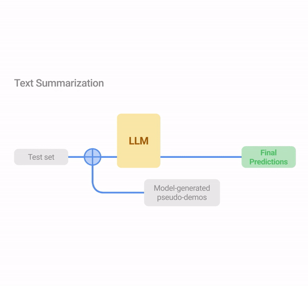
COSP focuses on question-answering tasks with CoT prompting for which it is easy to measure self-consistency since the questions have unique correct answers. But this can be difficult for other tasks, such as open-ended question-answering or generative tasks that don’t have unique answers (e.g., text summarization). To address this limitation, we introduce USP in which we generalize our approach to other general NLP tasks:

  • Classification (CLS): Problems where we can compute the probability of each class using the neural network output logits of each class. In this way, we can measure the uncertainty without multiple sampling by computing the entropy of the logit distribution.
  • Short-form generation (SFG): Problems like question answering where we can use the same procedure mentioned above for COSP, but, if necessary, without the rationale-generating step.
  • Long-form generation (LFG): Problems like summarization and translation, where the questions are often open-ended and the outputs are unlikely to be identical, even if the LLM is certain. In this case, we use an overlap metric in which we compute the average of the pairwise ROUGE score between the different outputs to the same query.
Illustration of USP in exemplary tasks (classification, QA and text summarization). Similar to COSP, the LLM first generates predictions on an unlabeled dataset whose outputs are scored with logit entropy, consistency or alignment, depending on the task type, and pseudo-demonstrations are selected from these input-output pairs. In Stage 2, the test instances are augmented with pseudo-demos for prediction.

We compute the relevant confidence scores depending on the type of task on the aforementioned set of unlabeled test samples. After scoring, similar to COSP, we pick the confident, diverse and less repetitive answers to form a model-generated pseudo-demonstration set. We finally query the LLM again in a few-shot format with these pseudo-demonstrations to obtain the final predictions on the entire test set.


Key Results

For COSP, we focus on a set of six arithmetic and commonsense reasoning problems, and we compare against 0-shot-CoT (i.e., “Let’s think step by step“ only). We use self-consistency in all baselines so that they use roughly the same amount of computational resources as COSP. Compared across three LLMs, we see that zero-shot COSP significantly outperforms the standard zero-shot baseline.

Key results of COSP in six arithmetic (MultiArith, GSM-8K, AddSub, SingleEq) and commonsense (CommonsenseQA, StrategyQA) reasoning tasks using PaLM-62B, PaLM-540B and GPT-3 (code-davinci-001) models.

USP improves significantly on 0-shot performance. “CLS” is an average of 15 classification tasks; “SFG” is the average of five short-form generation tasks; “LFG” is the average of two summarization tasks. “SFG (BBH)” is an average of all BIG-Bench Hard tasks, where each question is in SFG format.

For USP, we expand our analysis to a much wider range of tasks, including more than 25 classifications, short-form generation, and long-form generation tasks. Using the state-of-the-art PaLM 2 models, we also test against the BIG-Bench Hard suite of tasks where LLMs have previously underperformed compared to people. We show that in all cases, USP again outperforms the baselines and is competitive to prompting with golden examples.

Accuracy on BIG-Bench Hard tasks with PaLM 2-M (each line represents a task of the suite). The gain/loss of USP (green stars) over standard 0-shot (green triangles) is shown in percentages. “Human” refers to average human performance; “AutoCoT” and “Random demo” are baselines we compared against in the paper; and “3-shot” is the few-shot performance for three handcrafted demos in CoT format.

We also analyze the working mechanism of USP by validating the key observation above on the relation between confidence and correctness, and we found that in an overwhelming majority of the cases, USP picks confident predictions that are more likely better in all task types considered, as shown in the figure below.

USP picks confident predictions that are more likely better. Ground-truth performance metrics against USP confidence scores in selected tasks in various task types (blue: CLS, orange: SFG, green: LFG) with PaLM-540B.

Conclusion

Zero-shot inference is a highly sought-after capability of modern LLMs, yet the success in which poses unique challenges. We propose COSP and USP, a family of versatile, zero-shot automatic prompting techniques applicable to a wide range of tasks. We show large improvement over the state-of-the-art baselines over numerous task and model combinations.


Acknowledgements

This work was conducted by Xingchen Wan, Ruoxi Sun, Hootan Nakhost, Hanjun Dai, Julian Martin Eisenschlos, Sercan Ö. Arık, and Tomas Pfister. We would like to thank Jinsung Yoon Xuezhi Wang for providing helpful reviews, and other colleagues at Google Cloud AI Research for their discussion and feedback.

Source: Google AI Blog


MetNet-3: A state-of-the-art neural weather model available in Google products

Forecasting weather variables such as precipitation, temperature, and wind is key to numerous aspects of society, from daily planning and transportation to energy production. As we continue to see more extreme weather events such as floods, droughts, and heat waves, accurate forecasts can be essential to preparing for and mitigating their effects. The first 24 hours into the future are especially important as they are both highly predictable and actionable, which can help people make informed decisions in a timely manner and stay safe.

Today we present a new weather model called MetNet-3, developed by Google Research and Google DeepMind. Building on the earlier MetNet and MetNet-2 models, MetNet-3 provides high resolution predictions up to 24 hours ahead for a larger set of core variables, including precipitation, surface temperature, wind speed and direction, and dew point. MetNet-3 creates a temporally smooth and highly granular forecast, with lead time intervals of 2 minutes and spatial resolutions of 1 to 4 kilometers. MetNet-3 achieves strong performance compared to traditional methods, outperforming the best single- and multi-member physics-based numerical weather prediction (NWP) models — such as High-Resolution Rapid Refresh (HRRR) and ensemble forecast suite (ENS) — for multiple regions up to 24 hours ahead.

Finally, we’ve integrated MetNet-3’s capabilities across various Google products and technologies where weather is relevant. Currently available in the contiguous United States and parts of Europe with a focus on 12 hour precipitation forecasts, MetNet-3 is helping bring accurate and reliable weather information to people in multiple countries and languages.

     
MetNet-3 precipitation output summarized into actionable forecasts in Google Search on mobile.

Densification of sparse observations

Many recent machine learning weather models use the atmospheric state generated by traditional methods (e.g., data assimilation from NWPs) as the primary starting point to build forecasts. In contrast, a defining feature of the MetNet models has been to use direct observations of the atmosphere for training and evaluation. The advantage of direct observations is that they often have higher fidelity and resolution. However, direct observations come from a large variety of sensors at different altitudes, including weather stations at the surface level and satellites in orbit, and can be of varying degrees of sparsity. For example, precipitation estimates derived from radar such as NOAA’s Multi-Radar/Multi-Sensor System (MRMS) are relatively dense images, whereas weather stations located on the ground that provide measurements for variables such as temperature and wind are mere points spread over a region.

In addition to the data sources used in previous MetNet models, MetNet-3 includes point measurements from weather stations as both inputs and targets with the goal of making a forecast at all locations. To this end, MetNet-3’s key innovation is a technique called densification, which merges the traditional two-step process of data assimilation and simulation found in physics-based models into a single pass through the neural network. The main components of densification are illustrated below. Although the densification technique applies to a specific stream of data individually, the resulting densified forecast benefits from all the other input streams that go into MetNet-3, including topographical, satellite, radar, and NWP analysis features. No NWP forecasts are included in MetNet-3’s default inputs.

A) During training, a fraction of the weather stations are masked out from the input while kept in the target. B) To evaluate generalization to untrained locations, a set of weather stations represented by squares is never used for training and is only used for evaluation. C) Data from these held out weather stations with sparse coverage is included during evaluation to determine prediction quality in these areas. D) The final forecasts use the full set of training weather stations as input and produce fully dense forecasts aided by spatial parameter sharing.

High resolution in space and time

A central advantage of using direct observations is their high spatial and temporal resolution. For example, weather stations and ground radar stations provide measurements every few minutes at specific points and at 1 km resolutions, respectively; this is in stark contrast with the assimilation state from the state-of-the-art model ENS, which is generated every 6 hours at a resolution of 9 km with hour-by-hour forecasts. To handle such a high resolution, MetNet-3 preserves another of the defining features of this series of models, lead time conditioning. The lead time of the forecast in minutes is directly given as input to the neural network. This allows MetNet-3 to efficiently model the high temporal frequency of the observations for intervals as brief as 2 minutes. Densification combined with lead time conditioning and high resolution direct observations produces a fully dense 24 hour forecast with a temporal resolution of 2 minutes, while learning from just 1,000 points from the One Minute Observation (OMO) network of weather stations spread across the United States.

MetNet-3 predicts a marginal multinomial probability distribution for each output variable and each location that provides rich information beyond just the mean. This allows us to compare the probabilistic outputs of MetNet-3 with the outputs of advanced probabilistic ensemble NWP models, including the ensemble forecast ENS from the European Centre for Medium-Range Weather Forecasts and the High Resolution Ensemble Forecast (HREF) from the National Oceanic and Atmospheric Administration of the US. Due to the probabilistic nature of the outputs of both models, we are able to compute scores such as the Continuous Ranked Probability Score (CRPS). The following graphics highlight densification results and illustrate that MetNet’s forecasts are not only of much higher resolution, but are also more accurate when evaluated at the overlapping lead times.

Top: MetNet-3’s forecast of wind speed for each 2 minutes over the future 24 hours with a spatial resolution of 4km. Bottom: ENS’s hourly forecast with a spatial resolution of 18 km.
The two distinct regimes in spatial structure are primarily driven by the presence of the Colorado mountain ranges. Darker corresponds to higher wind speed. More samples available here: 1, 2, 3, 4.
Performance comparison between MetNet-3 and NWP baseline for wind speed based on CRPS (lower is better). In the hyperlocal setting, values of the test weather stations are given as input to the network during evaluation; the results improve further especially in the early lead times.

In contrast to weather station variables, precipitation estimates are more dense as they come from ground radar. MetNet-3’s modeling of precipitation is similar to that of MetNet-1 and 2, but extends the high resolution precipitation forecasts with a 1km spatial granularity to the same 24 hours of lead time as the other variables, as shown in the animation below. MetNet-3’s performance on precipitation achieves a better CRPS value than ENS’s throughout the 24 hour range.

Case study for Thu Jan 17 2019 00:00 UTC showing the probability of instantaneous precipitation rate being above 1 mm/h on CONUS. Darker corresponds to a higher probability value. The maps also show the prediction threshold when optimized towards Critical Success Index CSI (dark blue contours). This specific case study shows the formation of a new large precipitation pattern in the central US; it is not just forecasting of existing patterns.
Top: ENS’s hourly forecast. Center: Ground truth, source NOAA’s MRMS. Bottom: Probability map as predicted by MetNet-3. Native resolution available here.
Performance comparison between MetNet-3 and NWP baseline for instantaneous precipitation rate on CRPS (lower is better).

Delivering realtime ML forecasts

Training and evaluating a weather forecasting model like MetNet-3 on historical data is only a part of the process of delivering ML-powered forecasts to users. There are many considerations when developing a real-time ML system for weather forecasting, such as ingesting real-time input data from multiple distinct sources, running inference, implementing real-time validation of outputs, building insights from the rich output of the model that lead to an intuitive user experience, and serving the results at Google scale — all on a continuous cycle, refreshed every few minutes.

We developed such a real-time system that is capable of producing a precipitation forecast every few minutes for the entire contiguous United States and for 27 countries in Europe for a lead time of up to 12 hours.

Illustration of the process of generating precipitation forecasts using MetNet-3.

The system's uniqueness stems from its use of near-continuous inference, which allows the model to constantly create full forecasts based on incoming data streams. This mode of inference is different from traditional inference systems, and is necessary due to the distinct characteristics of the incoming data. The model takes in various data sources as input, such as radar, satellite, and numerical weather prediction assimilations. Each of these inputs has a different refresh frequency and spatial and temporal resolution. Some data sources, such as weather observations and radar, have characteristics similar to a continuous stream of data, while others, such as NWP assimilations, are similar to batches of data. The system is able to align all of these data sources spatially and temporally, allowing the model to create an updated understanding of the next 12 hours of precipitation at a very high cadence.

With the above process, the model is able to predict arbitrary discrete probability distributions. We developed novel techniques to transform this dense output space into user-friendly information that enables rich experiences throughout Google products and technologies.


Weather features in Google products

People around the world rely on Google every day to provide helpful, timely, and accurate information about the weather. This information is used for a variety of purposes, such as planning outdoor activities, packing for trips, and staying safe during severe weather events.

The state-of-the-art accuracy, high temporal and spatial resolution, and probabilistic nature of MetNet-3 makes it possible to create unique hyperlocal weather insights. For the contiguous United States and Europe, MetNet-3 is operational and produces real-time 12 hour precipitation forecasts that are now served across Google products and technologies where weather is relevant, such as Search. The rich output from the model is synthesized into actionable information and instantly served to millions of users.

For example, a user who searches for weather information for a precise location from their mobile device will receive highly localized precipitation forecast data, including timeline graphs with granular minute breakdowns depending on the product.

MetNet-3 precipitation output in weather on the Google app on Android (left) and mobile web Search (right).

Conclusion

MetNet-3 is a new deep learning model for weather forecasting that outperforms state-of-the-art physics-based models for 24-hour forecasts of a core set of weather variables. It has the potential to create new possibilities for weather forecasting and to improve the safety and efficiency of many activities, such as transportation, agriculture, and energy production. MetNet-3 is operational and its forecasts are served across several Google products where weather is relevant.


Acknowledgements

Many people were involved in the development of this effort. We would like to especially thank those from Google DeepMind (Di Li, Jeremiah Harmsen, Lasse Espeholt, Marcin Andrychowicz, Zack Ontiveros), Google Research (Aaron Bell, Akib Uddin, Alex Merose, Carla Bromberg, Fred Zyda, Isalo Montacute, Jared Sisk, Jason Hickey, Luke Barrington, Mark Young, Maya Tohidi, Natalie Williams, Pramod Gupta, Shreya Agrawal, Thomas Turnbull, Tom Small, Tyler Russell), and Google Search (Agustin Pesciallo, Bill Myers, Danny Cheresnick, Lior Cohen, Maca Piombi, Maia Diamant, Max Kamenetsky, Maya Ekron, Mor Schlesinger, Neta Gefen-Doron, Nofar Peled Levi, Ofer Lehr, Or Hillel, Rotem Wertman, Vinay Ruelius Shah, Yechie Labai).

Source: Google AI Blog


Looking back at wildfire research in 2023

Wildfires are becoming larger and affecting more and more communities around the world, often resulting in large-scale devastation. Just this year, communities have experienced catastrophic wildfires in Greece, Maui, and Canada to name a few. While the underlying causes leading to such an increase are complex — including changing climate patterns, forest management practices, land use development policies and many more — it is clear that the advancement of technologies can help to address the new challenges.

At Google Research, we’ve been investing in a number of climate adaptation efforts, including the application of machine learning (ML) to aid in wildfire prevention and provide information to people during these events. For example, to help map fire boundaries, our wildfire boundary tracker uses ML models and satellite imagery to map large fires in near real-time with updates every 15 minutes. To advance our various research efforts, we are partnering with wildfire experts and government agencies around the world.

Today we are excited to share more about our ongoing collaboration with the US Forest Service (USFS) to advance fire modeling tools and fire spread prediction algorithms. Starting from the newly developed USFS wildfire behavior model, we use ML to significantly reduce computation times, thus enabling the model to be employed in near real time. This new model is also capable of incorporating localized fuel characteristics, such as fuel type and distribution, in its predictions. Finally, we describe an early version of our new high-fidelity 3D fire spread model.


Current state of the art in wildfire modeling

Today’s most widely used state-of-the-art fire behavior models for fire operation and training are based on the Rothermel fire model developed at the US Forest Service Fire Lab, by Rothermel et al., in the 1970s. This model considers many key factors that affect fire spread, such as the influence of wind, the slope of the terrain, the moisture level, the fuel load (e.g., the density of the combustible materials in the forest), etc., and provided a good balance between computational feasibility and accuracy at the time. The Rothermel model has gained widespread use throughout the fire management community across the world.

Various operational tools that employ the Rothermel model, such as BEHAVE, FARSITE, FSPro, and FlamMap, have been developed and improved over the years. These tools and the underlying model are used mainly in three important ways: (1) for training firefighters and fire managers to develop their insights and intuitions on fire behavior, (2) for fire behavior analysts to predict the development of a fire during a fire operation and to generate guidance for situation awareness and resource allocation planning, and (3) for analyzing forest management options intended to mitigate fire hazards across large landscapes.  These models are the foundation of fire operation safety and efficiency today.

However, there are limitations on these state-of-the art models, mostly associated with the simplification of the underlying physical processes (which was necessary when these models were created). By simplifying the physics to produce steady state predictions, the required inputs for fuel sources and weather became practical but also more abstract compared to measurable quantities.  As a result, these models are typically “adjusted” and “tweaked” by experienced fire behavior analysts so they work more accurately in certain situations and to compensate for uncertainties and unknowable environmental characteristics. Yet these expert adjustments mean that many of the calculations are not repeatable.

To overcome these limitations, USFS researchers have been working on a new model to drastically improve the physical fidelity of fire behavior prediction. This effort represents the first major shift in fire modeling in the past 50 years. While the new model continues to improve in capturing fire behavior, the computational cost and inference time makes it impractical to be deployed in the field or for applications with near real-time requirements. In a realistic scenario, to make this model useful and practical in training and operations, a speed up of at least 1000x would be needed.


Machine learning acceleration

In partnership with the USFS, we have undertaken a program to apply ML to decrease computation times for complex fire models. Researchers knew that many complex inputs and features could be characterized using a deep neural network, and if successful, the trained model would lower the computational cost and latency of evaluating new scenarios. Deep learning is a branch of machine learning that uses neural networks with multiple hidden layers of nodes that do not directly correspond to actual observations. The model’s hidden layers allow a rich representation of extremely complex systems — an ideal technique for modeling wildfire spread.

We used the USFS physics-based, numerical prediction models to generate many simulations of wildfire behavior and then used these simulated examples to train the deep learning model on the inputs and features to best capture the system behavior accurately. We found that the deep learning model can perform at a much lower computational cost compared to the original and is able to address behaviors resulting from fine-scale processes. In some cases, computation time for capturing the fine-scale features described above and providing a fire spread estimate was 100,000 times faster than running the physics-based numerical models.

This project has continued to make great progress since the first report at presentation at ICFFR 2022 and the USFS Fire Lab's project page provides a glimpse into the ongoing work in this direction. Our team has expanded the dataset used for training by an order of magnitude, from 40M up to 550M training examples. Additionally, we have delivered a prototype ML model that our USFS Fire Lab partner is integrating into a training app that is currently being developed for release in 2024.

Google researchers visiting the USFS Fire Lab in Missoula, MT, stopping by Big Knife Fire Operation Command Center.

Fine-grained fuel representation

Besides training, another key use-case of the new model is for operational fire prediction. To fully leverage the advantages of the new model’s capability to capture the detailed fire behavior changes from small-scale differences in fuel structures, high resolution fuel mapping and representation are needed. To this end, we are currently working on the integration of high resolution satellite imagery and geo information into ML models to allow fuel specific mapping at-scale. Some of the preliminary results will be presented at the upcoming 10th International Fire Ecology and Management Congress in November 2023.


Future work

Beyond the collaboration on the new fire spread model, there are many important and challenging problems that can help fire management and safety. Many such problems require even more accurate fire models that fully consider 3D flow interactions and fluid dynamics, thermodynamics and combustion physics. Such detailed calculations usually require high-performance computers (HPCs) or supercomputers.

These models can be used for research and longer-term planning purposes to develop insights on extreme fire development scenarios, build ML classification models, or establish a meaningful “danger index” using the simulated results. These high-fidelity simulations can also be used to supplement physical experiments that are used in expanding the operational models mentioned above.

In this direction, Google research has also developed a high-fidelity large-scale 3D fire simulator that can be run on Google TPUs. In the near future, there is a plan to further leverage this new capability to augment the experiments, and to generate data to build insights on the development of extreme fires and use the data to design a fire-danger classifier and fire-danger index protocol.

An example of 3D high-fidelity simulation. This is a controlled burn field experiment (FireFlux II) simulated using Google’s high fidelity fire simulator.

Acknowledgements

We thank Mark Finney, Jason Forthofer, William Chatham and Issac Grenfell from US Forest Service Missoula Fire Science Laboratory and our colleagues John Burge, Lily Hu, Qing Wang, Cenk Gazen, Matthias Ihme, Vivian Yang, Fei Sha and John Anderson for core contributions and useful discussions. We also thank Tyler Russell for his assistance with program management and coordination.

Source: Google AI Blog


Batch calibration: Rethinking calibration for in-context learning and prompt engineering

Prompting large language models (LLMs) has become an efficient learning paradigm for adapting LLMs to a new task by conditioning on human-designed instructions. The remarkable in-context learning (ICL) ability of LLMs also leads to efficient few-shot learners that can generalize from few-shot input-label pairs. However, the predictions of LLMs are highly sensitive and even biased to the choice of templates, label spaces (such as yes/no, true/false, correct/incorrect), and demonstration examples, resulting in unexpected performance degradation and barriers for pursuing robust LLM applications. To address this problem, calibration methods have been developed to mitigate the effects of these biases while recovering LLM performance. Though multiple calibration solutions have been provided (e.g., contextual calibration and domain-context calibration), the field currently lacks a unified analysis that systematically distinguishes and explains the unique characteristics, merits, and downsides of each approach.

With this in mind, in “Batch Calibration: Rethinking Calibration for In-Context Learning and Prompt Engineering”, we conduct a systematic analysis of the existing calibration methods, where we both provide a unified view and reveal the failure cases. Inspired by these analyses, we propose Batch Calibration (BC), a simple yet intuitive method that mitigates the bias from a batch of inputs, unifies various prior approaches, and effectively addresses the limitations in previous methods. BC is zero-shot, self-adaptive (i.e., inference-only), and incurs negligible additional costs. We validate the effectiveness of BC with PaLM 2 and CLIP models and demonstrate state-of-the-art performance over previous calibration baselines across more than 10 natural language understanding and image classification tasks.


Motivation

In pursuit of practical guidelines for ICL calibration, we started with understanding the limitations of current methods. We find that the calibration problem can be framed as an unsupervised decision boundary learning problem. We observe that uncalibrated ICL can be biased towards predicting a class, which we explicitly refer to as contextual bias, the a priori propensity of LLMs to predict certain classes over others unfairly given the context. For example, the prediction of LLMs can be biased towards predicting the most frequent label, or the label towards the end of the demonstration. We find that, while theoretically more flexible, non-linear boundaries (prototypical calibration) tend to be susceptible to overfitting and may suffer from instability for challenging multi-class tasks. Conversely, we find that linear decision boundaries can be more robust and generalizable across tasks. In addition, we find that relying on additional content-free inputs (e.g., “N/A” or random in-domain tokens) as the grounds for estimating the contextual bias is not always optimal and may even introduce additional bias, depending on the task type.


Batch calibration

Inspired by the previous discussions, we designed BC to be a zero-shot, inference-only and generalizable calibration technique with negligible computation cost. We argue that the most critical component for calibration is to accurately estimate the contextual bias. We, therefore, opt for a linear decision boundary for its robustness, and instead of relying on content-free inputs, we propose to estimate the contextual bias for each class from a batch in a content-based manner by marginalizing the output score over all samples within the batch, which is equivalent to measuring the mean score for each class (visualized below).

We then obtain the calibrated probability by dividing the output probability over the contextual prior, which is equivalent to aligning the log-probability (LLM scores) distribution to the estimated mean of each class. It is noteworthy that because it requires no additional inputs to estimate the bias, this BC procedure is zero-shot, only involves unlabeled test samples, and incurs negligible computation costs. We may either compute the contextual bias once all test samples are seen, or alternatively, in an on-the-fly manner that dynamically processes the outputs. To do so, we may use a running estimate of the contextual bias for BC, thereby allowing BC's calibration term to be estimated from a small number of mini-batches that is subsequently stabilized when more mini-batches arrive.

Illustration of Batch Calibration (BC). Batches of demonstrations with in-context examples and test samples are passed into the LLM. Due to sources of implicit bias in the context, the score distribution from the LLM becomes biased. BC is a modular and adaptable layer option appended to the output of the LLM that generates calibrated scores (visualized for illustration only).

Experiment design

For natural language tasks, we conduct experiments on 13 more diverse and challenging classification tasks, including the standard GLUE and SuperGLUE datasets. This is in contrast to previous works that only report on relatively simple single-sentence classification tasks.. For image classification tasks, we include SVHN, EuroSAT, and CLEVR. We conduct experiments mainly on the state-of-the-art PaLM 2 with size variants PaLM 2-S, PaLM 2-M, and PaLM 2-L. For VLMs, we report the results on CLIP ViT-B/16.


Results

Notably, BC consistently outperforms ICL, yielding a significant performance enhancement of 8% and 6% on small and large variants of PaLM 2, respectively. This shows that the BC implementation successfully mitigates the contextual bias from the in-context examples and unleashes the full potential of LLM in efficient learning and quick adaptation to new tasks. In addition, BC improves over the state-of-the-art prototypical calibration (PC) baseline by 6% on PaLM 2-S, and surpasses the competitive contextual calibration (CC) baseline by another 3% on average on PaLM 2-L. Specifically, BC is a generalizable and cheaper technique across all evaluated tasks, delivering stable performance improvement, whereas previous baselines exhibit varying degrees of performance across tasks.

Batch Calibration (BC) achieves the best performance on 1-shot ICL over calibration baselines: contextual calibration (CC), domain-context calibration (DC), and prototypical calibration (PC) on an average of 13 NLP tasks on PaLM 2 and outperforms the zero-shot CLIP on image tasks.

We analyze the performance of BC by varying the number of ICL shots from 0 to 4, and BC again outperforms all baseline methods. We also observe an overall trend for improved performance when more shots are available, where BC demonstrates the best stability.

The ICL performance on various calibration techniques over the number of ICL shots on PaLM 2-S. We compare BC with the uncalibrated ICL, contextual calibration (CC), domain-context calibration (DC), and prototypical calibration (PC) baselines.

We further visualize the decision boundaries of uncalibrated ICL after applying existing calibration methods and the proposed BC. We show success and failure cases for each baseline method, whereas BC is consistently effective.

Visualization of the decision boundaries of uncalibrated ICL, and after applying existing calibration methods and the proposed BC in representative binary classification tasks of SST-2 (top row) and QNLI (bottom row) on 1-shot PaLM 2-S. Each axis indicates the LLM score on the defined label.

Robustness and ablation studies

We analyze the robustness of BC with respect to common prompt engineering design choices that were previously shown to significantly affect LLM performance: choices and orders of in-context examples, the prompt template for ICL, and the label space. First, we find that BC is more robust to ICL choices and can mostly achieve the same performance with different ICL examples. Additionally, given a single set of ICL shots, altering the order between each ICL example has minimal impact on the BC performance. Furthermore, we analyze the robustness of BC under 10 designs of prompt templates, where BC shows consistent improvement over the ICL baseline. Therefore, though BC improves performance, a well-designed template can further enhance the performance of BC. Lastly, we examine the robustness of BC to variations in label space designs (see appendix in our paper). Remarkably, even when employing unconventional choices such as emoji pairs as labels, leading to dramatic oscillations of ICL performance, BC largely recovers performance. This observation demonstrates that BC increases the robustness of LLM predictions under common prompt design choices and makes prompt engineering easier.

Batch Calibration makes prompt engineering easier while being data-efficient. Data are visualized as a standard box plot, which illustrates values for the median, first and third quartiles, and minimum and maximum.

Moreover, we study the impact of batch size on the performance of BC. In contrast to PC, which also leverages an unlabeled estimate set, BC is remarkably more sample efficient, achieving a strong performance with only around 10 unlabeled samples, whereas PC requires more than 500 unlabeled samples before its performance stabilizes.

Batch Calibration makes prompt engineering easier while being insensitive to the batch size.

Conclusion

We first revisit previous calibration methods while addressing two critical research questions from an interpretation of decision boundaries, revealing their failure cases and deficiencies. We then propose Batch Calibration, a zero-shot and inference-only calibration technique. While methodologically simple and easy to implement with negligible computation cost, we show that BC scales from a language-only setup to the vision-language context, achieving state-of-the-art performance in both modalities. BC significantly improves the robustness of LLMs with respect to prompt designs, and we expect easy prompt engineering with BC.


Acknowledgements

This work was conducted by Han Zhou, Xingchen Wan, Lev Proleev, Diana Mincu, Jilin Chen, Katherine Heller, Subhrajit Roy. We would like to thank Mohammad Havaei and other colleagues at Google Research for their discussion and feedback.

Source: Google AI Blog


7 dos and don’ts of using ML on the web with MediaPipe

Posted by Jen Person, Developer Relations Engineer

If you're a web developer looking to bring the power of machine learning (ML) to your web apps, then check out MediaPipe Solutions! With MediaPipe Solutions, you can deploy custom tasks to solve common ML problems in just a few lines of code. View the guides in the docs and try out the web demos on Codepen to see how simple it is to get started. While MediaPipe Solutions handles a lot of the complexity of ML on the web, there are still a few things to keep in mind that go beyond the usual JavaScript best practices. I've compiled them here in this list of seven dos and don'ts. Do read on to get some good tips!


❌ DON'T bundle your model in your app

As a web developer, you're accustomed to making your apps as lightweight as possible to ensure the best user experience. When you have larger items to load, you already know that you want to download them in a thoughtful way that allows the user to interact with the content quickly rather than having to wait for a long download. Strategies like quantization have made ML models smaller and accessible to edge devices, but they're still large enough that you don't want to bundle them in your web app. Store your models in the cloud storage solution of your choice. Then, when you initialize your task, the model and WebAssembly binary will be downloaded and initialized. After the first page load, use local storage or IndexedDB to cache the model and binary so future page loads run even faster. You can see an example of this in this touchless ATM sample app on GitHub.


✅ DO initialize your task early

Task initialization can take a bit of time depending on model size, connection speed, and device type. Therefore, it's a good idea to initialize the solution before user interaction. In the majority of the code samples on Codepen, initialization takes place on page load. Keep in mind that these samples are meant to be as simple as possible so you can understand the code and apply it to your own use case. Initializing your model on page load might not make sense for you. Just focus on finding the right place to spin up the task so that processing is hidden from the user.

After initialization, you should warm up the task by passing a placeholder image through the model. This example shows a function for running a 1x1 pixel canvas through the Pose Landmarker task:

function dummyDetection(poseLandmarker: PoseLandmarker) { const width = 1; const height = 1; const canvas = document.createElement('canvas'); canvas.width = width; canvas.height = height; const ctx = canvas.getContext('2d'); ctx.fillStyle = 'rgba(0, 0, 0, 1)'; ctx.fillRect(0, 0, width, height); poseLandmarker.detect(canvas); }


✅ DO clean up resources

One of my favorite parts of JavaScript is automatic garbage collection. In fact, I can't remember the last time memory management crossed my mind. Hopefully you've cached a little information about memory in your own memory, as you'll need just a bit of it to make the most of your MediaPipe task. MediaPipe Solutions for web uses WebAssembly (WASM) to run C++ code in-browser. You don't need to know C++, but it helps to know that C++ makes you take out your own garbage. If you don't free up unused memory, you will find that your web page uses more and more memory over time. It can have performance issues or even crash.

When you're done with your solution, free up resources using the .close() method.

For example, I can create a gesture recognizer using the following code:

const createGestureRecognizer = async () => { const vision = await FilesetResolver.forVisionTasks( "https://cdn.jsdelivr.net/npm/@mediapipe/[email protected]/wasm" ); gestureRecognizer = await GestureRecognizer.createFromOptions(vision, { baseOptions: { modelAssetPath: "https://storage.googleapis.com/mediapipe-models/gesture_recognizer/gesture_recognizer/float16/1/gesture_recognizer.task", delegate: "GPU" }, }); }; createGestureRecognizer();

Once I'm done recognizing gestures, I dispose of the gesture recognizer using the close() method:

gestureRecognizer.close();

Each task has a close method, so be sure to use it where relevant! Some tasks have close() methods for the returned results, so refer to the API docs for details.


✅ DO try out tasks in MediaPipe Studio

When deciding on or customizing your solution, it's a good idea to try it out in MediaPipe Studio before writing your own code. MediaPipe Studio is a web-based application for evaluating and customizing on-device ML models and pipelines for your applications. The app lets you quickly test MediaPipe solutions in your browser with your own data, and your own customized ML models. Each solution demo also lets you experiment with model settings for the total number of results, minimum confidence threshold for reporting results, and more. You'll find this especially useful when customizing solutions so you can see how your model performs without needing to create a test web page.

Screenshot of Image Classification page in MediaPipe Studio


✅ DO test on different devices

It's always important to test your web apps on various devices and browsers to ensure they work as expected, but I think it's worth adding a reminder here to test early and often on a variety of platforms. You can use MediaPipe Studio to test devices as well so you know right away that a solution will work on your users' devices.


❌ DON'T default to the biggest model

Each task lists one or more recommended models. For example, the Object Detection task lists three different models, each with benefits and drawbacks based on speed, size and accuracy. It can be tempting to think that the most important thing is to choose the model with the very highest accuracy, but if you do so, you will be sacrificing speed and increasing the size of your model. Depending on your use case, your users might benefit from a faster result rather than a more accurate one. The best way to compare model options is in MediaPipe Studio. I realize that this is starting to sound like an advertisement for MediaPipe Studio, but it really does come in handy here!

photo of a whale breeching against a background of clouds in a deep, vibrant blue sky

✅ DO reach out!

Do you have any dos or don'ts of ML on the web that you think I missed? Do you have questions about how to get started? Or do you have a cool project you want to share? Reach out to me on LinkedIn and tell me all about it!

Re-weighted gradient descent via distributionally robust optimization

Deep neural networks (DNNs) have become essential for solving a wide range of tasks, from standard supervised learning (image classification using ViT) to meta-learning. The most commonly-used paradigm for learning DNNs is empirical risk minimization (ERM), which aims to identify a network that minimizes the average loss on training data points. Several algorithms, including stochastic gradient descent (SGD), Adam, and Adagrad, have been proposed for solving ERM. However, a drawback of ERM is that it weights all the samples equally, often ignoring the rare and more difficult samples, and focusing on the easier and abundant samples. This leads to suboptimal performance on unseen data, especially when the training data is scarce.

To overcome this challenge, recent works have developed data re-weighting techniques for improving ERM performance. However, these approaches focus on specific learning tasks (such as classification) and/or require learning an additional meta model that predicts the weights of each data point. The presence of an additional model significantly increases the complexity of training and makes them unwieldy in practice.

In “Stochastic Re-weighted Gradient Descent via Distributionally Robust Optimization” we introduce a variant of the classical SGD algorithm that re-weights data points during each optimization step based on their difficulty. Stochastic Re-weighted Gradient Descent (RGD) is a lightweight algorithm that comes with a simple closed-form expression, and can be applied to solve any learning task using just two lines of code. At any stage of the learning process, RGD simply reweights a data point as the exponential of its loss. We empirically demonstrate that the RGD reweighting algorithm improves the performance of numerous learning algorithms across various tasks, ranging from supervised learning to meta learning. Notably, we show improvements over state-of-the-art methods on DomainBed and Tabular classification. Moreover, the RGD algorithm also boosts performance for BERT using the GLUE benchmarks and ViT on ImageNet-1K.


Distributionally robust optimization

Distributionally robust optimization (DRO) is an approach that assumes a “worst-case” data distribution shift may occur, which can harm a model's performance. If a model has focussed on identifying few spurious features for prediction, these “worst-case” data distribution shifts could lead to the misclassification of samples and, thus, a performance drop. DRO optimizes the loss for samples in that “worst-case” distribution, making the model robust to perturbations (e.g., removing a small fraction of points from a dataset, minor up/down weighting of data points, etc.) in the data distribution. In the context of classification, this forces the model to place less emphasis on noisy features and more emphasis on useful and predictive features. Consequently, models optimized using DRO tend to have better generalization guarantees and stronger performance on unseen samples.

Inspired by these results, we develop the RGD algorithm as a technique for solving the DRO objective. Specifically, we focus on Kullback–Leibler divergence-based DRO, where one adds perturbations to create distributions that are close to the original data distribution in the KL divergence metric, enabling a model to perform well over all possible perturbations.

Figure illustrating DRO. In contrast to ERM, which learns a model that minimizes expected loss over original data distribution, DRO learns a model that performs well on several perturbed versions of the original data distribution.


Stochastic re-weighted gradient descent

Consider a random subset of samples (called a mini-batch), where each data point has an associated loss Li. Traditional algorithms like SGD give equal importance to all the samples in the mini-batch, and update the parameters of the model by descending along the averaged gradients of the loss of those samples. With RGD, we reweight each sample in the mini-batch and give more importance to points that the model identifies as more difficult. To be precise, we use the loss as a proxy to calculate the difficulty of a point, and reweight it by the exponential of its loss. Finally, we update the model parameters by descending along the weighted average of the gradients of the samples.

Due to stability considerations, in our experiments we clip and scale the loss before computing its exponential. Specifically, we clip the loss at some threshold T, and multiply it with a scalar that is inversely proportional to the threshold. An important aspect of RGD is its simplicity as it doesn’t rely on a meta model to compute the weights of data points. Furthermore, it can be implemented with two lines of code, and combined with any popular optimizers (such as SGD, Adam, and Adagrad.

Figure illustrating the intuitive idea behind RGD in a binary classification setting. Feature 1 and Feature 2 are the features available to the model for predicting the label of a data point. RGD upweights the data points with high losses that have been misclassified by the model.


Results

We present empirical results comparing RGD with state-of-the-art techniques on standard supervised learning and domain adaptation (refer to the paper for results on meta learning). In all our experiments, we tune the clipping level and the learning rate of the optimizer using a held-out validation set.


Supervised learning

We evaluate RGD on several supervised learning tasks, including language, vision, and tabular classification. For the task of language classification, we apply RGD to the BERT model trained on the General Language Understanding Evaluation (GLUE) benchmark and show that RGD outperforms the BERT baseline by +1.94% with a standard deviation of 0.42%. To evaluate RGD’s performance on vision classification, we apply RGD to the ViT-S model trained on the ImageNet-1K dataset, and show that RGD outperforms the ViT-S baseline by +1.01% with a standard deviation of 0.23%. Moreover, we perform hypothesis tests to confirm that these results are statistically significant with a p-value that is less than 0.05.

RGD’s performance on language and vision classification using GLUE and Imagenet-1K benchmarks. Note that MNLI, QQP, QNLI, SST-2, MRPC, RTE and COLA are diverse datasets which comprise the GLUE benchmark.

For tabular classification, we use MET as our baseline, and consider various binary and multi-class datasets from UC Irvine's machine learning repository. We show that applying RGD to the MET framework improves its performance by 1.51% and 1.27% on binary and multi-class tabular classification, respectively, achieving state-of-the-art performance in this domain.


Performance of RGD for classification of various tabular datasets.


Domain generalization

To evaluate RGD’s generalization capabilities, we use the standard DomainBed benchmark, which is commonly used to study a model’s out-of-domain performance. We apply RGD to FRR, a recent approach that improved out-of-domain benchmarks, and show that RGD with FRR performs an average of 0.7% better than the FRR baseline. Furthermore, we confirm with hypothesis tests that most benchmark results (except for Office Home) are statistically significant with a p-value less than 0.05.

Performance of RGD on DomainBed benchmark for distributional shifts.


Class imbalance and fairness

To demonstrate that models learned using RGD perform well despite class imbalance, where certain classes in the dataset are underrepresented, we compare RGD’s performance with ERM on long-tailed CIFAR-10. We report that RGD improves the accuracy of baseline ERM by an average of 2.55% with a standard deviation of 0.23%. Furthermore, we perform hypothesis tests and confirm that these results are statistically significant with a p-value of less than 0.05.

Performance of RGD on the long-tailed Cifar-10 benchmark for class imbalance domain.


Limitations

The RGD algorithm was developed using popular research datasets, which were already curated to remove corruptions (e.g., noise and incorrect labels). Therefore, RGD may not provide performance improvements in scenarios where training data has a high volume of corruptions. A potential approach to handle such scenarios is to apply an outlier removal technique to the RGD algorithm. This outlier removal technique should be capable of filtering out outliers from the mini-batch and sending the remaining points to our algorithm.


Conclusion

RGD has been shown to be effective on a variety of tasks, including out-of-domain generalization, tabular representation learning, and class imbalance. It is simple to implement and can be seamlessly integrated into existing algorithms with just two lines of code change. Overall, RGD is a promising technique for boosting the performance of DNNs, and could help push the boundaries in various domains.


Acknowledgements

The paper described in this blog post was written by Ramnath Kumar, Arun Sai Suggala, Dheeraj Nagaraj and Kushal Majmundar. We extend our sincere gratitude to the anonymous reviewers, Prateek Jain, Pradeep Shenoy, Anshul Nasery, Lovish Madaan, and the numerous dedicated members of the machine learning and optimization team at Google Research India for their invaluable feedback and contributions to this work.

Source: Google AI Blog


Google Research embarks on effort to map a mouse brain

The human brain is perhaps the most computationally complex machine in existence, consisting of networks of billions of cells. Researchers currently don’t understand the full picture of how glitches in its network machinery contribute to mental illnesses and other diseases, such as dementia. However, the emerging connectomics field, which aims to precisely map the connections between every cell in the brain, could help solve that problem. While maps have only been created for simpler organisms, technological advances for mapping even larger brains can enable us to understand how the human brain works, and how to treat brain diseases.

Today, we're excited to announce that the Connectomics team at Google Research and our collaborators are launching a $33 million project to expand the frontiers of connectomics over the next five years. Supported by the Brain Research Through Advancing Innovative Neurotechnologies (BRAIN) Initiative at the National Institutes of Health (NIH) and led by researchers at Harvard University, we'll be working alongside a multidisciplinary team of experts from the Allen Institute, MIT, Cambridge University, Princeton University and Johns Hopkins University, with advisers from HHMI’s Janelia Research Campus. Our project goal is to tackle an immense challenge in neuroscience: mapping a tiny fraction (2-3%) of the mouse brain. We will specifically target the hippocampal region, which is responsible for encoding memories, attention and spatial navigation. This project is one of 11 funded by the NIH's $150 million BRAIN Initiative Connectivity Across Scales (BRAIN CONNECTS) program. Google Research is contributing computational and analytical resources to this effort, and will not receive any funding from the NIH. Our project asks a critical question: Can we scale and speed up our technologies enough to map the whole connectome of a mouse brain?


The modern era of connectomics

This effort to map the connectome of a small part of the mouse brain builds on a decade of innovation in the field, including many advances initiated by the Connectomics team at Google Research. We hope to accomplish something similar to the early days of the Human Genome Project, when scientists worked for years to sequence a small portion of the human genome as they refined technologies that would enable them to complete the rest of the genome.

In 2021, we and collaborators at Harvard successfully mapped one cubic millimeter of the human brain, which we released as the H01 dataset, a resource for studying the human brain and scaling connectomics technologies. But mapping the entire human brain connectome would require gathering and analyzing as much as a zettabyte of data (one billion terabytes), which is beyond the current capabilities of existing technologies.

Analyzing a mouse connectome is the next best thing. It is small enough to be technically feasible and could potentially deliver insights relevant to our own minds; neuroscientists already use mice to study human brain function and dysfunction. By working together to map 10–15 cubic mm of the mouse brain, we hope to develop new approaches that will allow us to map the entire remainder of the mouse brain, and the human brain thereafter.

Neuroscientists have been working for decades to map increasingly larger and more complicated connectomes.


One of biology’s largest datasets

In this connectomics project, we will map the connectome of the hippocampal formation of the mouse brain, which converts short-term memories into long-term memories and helps the mouse navigate in space. The mouse hippocampal formation is the largest area of any brain we’ve attempted to understand in this way. Through mapping this region of the mouse brain, we will create one of the largest datasets in biology, combining about 25,000 terabytes, or 25 petabytes of brain data. For reference, there are about 250 billion stars in our Milky Way Galaxy. If each of those stars was a single byte, it would take 100,000 Milky Way Galaxies to match the 25 petabytes of data that the project will collect when mapping a small region of the mouse brain.

To illustrate the hippocampal project’s scale, we calculated the number of Pixel phones (shown as stacks of Pixels below) needed to store the image data from the completed connectome projects that mapped the roundworm and fruit fly brains, as well as for the mouse hippocampal region and entire mouse brain projects, which are just getting started.

Then, we compared the heights of each Pixel stack to familiar objects and landmarks. It would take a stack of 100 Pixels, as tall as a four-year-old girl, to store the image data for the fruit fly brain, the largest completed project thus far. In contrast, the mouse hippocampal connectome effort will require storage equivalent to more than 48,800 Pixels, reaching as high as the Empire State Building. The animation below shows how the mouse hippocampal project will surpass the scale of previous connectome projects.

We are partnering with several collaborators to build a connectome (a map of the connections between brain cells) for the hippocampal region of a mouse brain. This project will create the largest connectomic dataset ever, surpassing the scale of previous projects that mapped the smaller roundworm and fruit fly brains. We hope this effort will lead to the development of new approaches that will allow us to later map an entire mouse brain. This animation shows how the field of connectomics is scaling up by calculating the number of Pixel phones needed to store the data from various projects. It would take just two Pixels, the height of an olive, to store the roundworm connectome data, while it would take a stack of Pixels the size of Mount Everest to store the data from an entire mouse connectome.

Understanding the connectome of the mouse hippocampal formation could help illuminate the way our own brains work. For instance, we may find common features between this circuitry in the mouse brain and human brains that explain how we know where we are, how our brains associate memories with specific locations, and what goes wrong in people who can’t properly form new spatial memories.


Opening the petabyte pipeline

Over the last decade, our team has worked to develop tools for managing massive connectomic datasets, and extracting scientific value from them. But a mouse brain has 1,000 times more neurons than the brain of the Drosophila fruit fly, an organism for which we helped build a connectome for a large part of the brain. Starting the mouse brain connectome will challenge us to improve existing technologies to enable us to map more data faster than ever before.

We’ll continue to refine our flood-filling networks, which use deep learning to trace, or “segment”, each neuron’s path through three-dimensional brain volumes made from electron microscope data. We’ll also extend the capabilities of our self-supervised learning technology, SegCLR, which allows us to automatically extract key insights from segmented volumes, such as identifying cell type (e.g., pyramidal neuron, basket neuron, etc.) and parts of each neuron (e.g., axon, dendrite, etc.).

A flood filling network traces a neuron through three-dimensional brain space.

We will also continue to enhance the scalability and performance of our core connectomics infrastructure, such as TensorStore for storage and Neuroglancer for visualization, in order to enable all of our computational pipelines and human analysis workflows to operate at these new scales of data. We’re eager to get to work to discover what peering into a mouse’s mind might tell us about our own.


Acknowledgements

The mouse connectomics project described in this blog post will be supported in part by the NIH BRAIN Initiative under award number 1UM1NS132250. Google Research is contributing computational and analytical resources to the mouse connectome project, and will not receive funding from the NIH. Many people were involved in the development of the technologies that make this project possible. We thank our long-term academic collaborators in the Lichtman Lab (Harvard University), HHMI Janelia, and the Denk Lab (Max Planck Institute for Biological Intelligence), and acknowledge core contributions from the Connectomics Team at Google. We also thank John Guilyard for creating the illustrative animation in this post, and Elise Kleeman, and Erika Check Hayden for their support. Thanks to Lizzie Dorfman, Michael Brenner, Jay Yagnik and Jeff Dean for their support, coordination and leadership.

Source: Google AI Blog


Distilling step-by-step: Outperforming larger language models with less training data and smaller model sizes

Large language models (LLMs) have enabled a new data-efficient learning paradigm wherein they can be used to solve unseen new tasks via zero-shot or few-shot prompting. However, LLMs are challenging to deploy for real-world applications due to their sheer size. For instance, serving a single 175 billion LLM requires at least 350GB of GPU memory using specialized infrastructure, not to mention that today's state-of-the-art LLMs are composed of over 500 billion parameters. Such computational requirements are inaccessible for many research teams, especially for applications that require low latency performance.

To circumvent these deployment challenges, practitioners often choose to deploy smaller specialized models instead. These smaller models are trained using one of two common paradigms: fine-tuning or distillation. Fine-tuning updates a pre-trained smaller model (e.g., BERT or T5) using downstream manually-annotated data. Distillation trains the same smaller models with labels generated by a larger LLM. Unfortunately, to achieve comparable performance to LLMs, fine-tuning methods require human-generated labels, which are expensive and tedious to obtain, while distillation requires large amounts of unlabeled data, which can also be hard to collect.

In “Distilling Step-by-Step! Outperforming Larger Language Models with Less Training Data and Smaller Model Sizes”, presented at ACL2023, we set out to tackle this trade-off between model size and training data collection cost. We introduce distilling step-by-step, a new simple mechanism that allows us to train smaller task-specific models with much less training data than required by standard fine-tuning or distillation approaches that outperform few-shot prompted LLMs’ performance. We demonstrate that the distilling step-by-step mechanism enables a 770M parameter T5 model to outperform the few-shot prompted 540B PaLM model using only 80% of examples in a benchmark dataset, which demonstrates a more than 700x model size reduction with much less training data required by standard approaches.

While LLMs offer strong zero and few-shot performance, they are challenging to serve in practice. On the other hand, traditional ways of training small task-specific models require a large amount of training data. Distilling step-by-step provides a new paradigm that reduces both the deployed model size as well as the number of data required for training.


Distilling step-by-step

The key idea of distilling step-by-step is to extract informative natural language rationales (i.e., intermediate reasoning steps) from LLMs, which can in turn be used to train small models in a more data-efficient way. Specifically, natural language rationales explain the connections between the input questions and their corresponding outputs. For example, when asked, “Jesse's room is 11 feet long and 15 feet wide. If she already has 16 square feet of carpet, how much more carpet does she need to cover the whole floor?”, an LLM can be prompted by the few-shot chain-of-thought (CoT) prompting technique to provide intermediate rationales, such as, “Area = length * width. Jesse’s room has 11 * 15 square feet.” That better explains the connection from the input to the final answer, “(11 * 15 ) - 16”. These rationales can contain relevant task knowledge, such as “Area = length * width”, that may originally require many data for small models to learn. We utilize these extracted rationales as additional, richer supervision to train small models, in addition to the standard task labels.

Overview on distilling step-by-step: First, we utilize CoT prompting to extract rationales from an LLM. We then use the generated rationales to train small task-specific models within a multi-task learning framework, where we prepend task prefixes to the input examples and train the model to output differently based on the given task prefix.

Distilling step-by-step consists of two main stages. In the first stage, we leverage few-shot CoT prompting to extract rationales from LLMs. Specifically, given a task, we prepare few-shot exemplars in the LLM input prompt where each example is composed of a triplet containing: (1) input, (2) rationale, and (3) output. Given the prompt, an LLM is able to mimic the triplet demonstration to generate the rationale for any new input. For instance, in a commonsense question answering task, given the input question “Sammy wanted to go to where the people are. Where might he go? Answer Choices: (a) populated areas, (b) race track, (c) desert, (d) apartment, (e) roadblock”, distilling step-by-step provides the correct answer to the question, “(a) populated areas”, paired with the rationale that provides better connection from the question to the answer, “The answer must be a place with a lot of people. Of the above choices, only populated areas have a lot of people.” By providing CoT examples paired with rationales in the prompt, the in-context learning ability allows LLMs to output corresponding rationales for future unseen inputs.

We use the few-shot CoT prompting, which contains both an example rationale (highlighted in green) and a label (highlighted in blue), to elicit rationales from an LLM on new input examples. The example is from a commonsense question answering task.

After the rationales are extracted, in the second stage, we incorporate the rationales in training small models by framing the training process as a multi-task problem. Specifically, we train the small model with a novel rationale generation task in addition to the standard label prediction task. The rationale generation task enables the model to learn to generate the intermediate reasoning steps for the prediction, and guides the model to better predict the resultant label. We prepend task prefixes (i.e., [label] and [rationale] for label prediction and rationale generation, respectively) to the input examples for the model to differentiate the two tasks.


Experimental setup

In the experiments, we consider a 540B PaLM model as the LLM. For task-specific downstream models, we use T5 models. For CoT prompting, we use the original CoT prompts when available and curate our own examples for new datasets. We conduct the experiments on four benchmark datasets across three different NLP tasks: e-SNLI and ANLI for natural language inference; CQA for commonsense question answering; and SVAMP for arithmetic math word problems. We include two sets of baseline methods. For comparison to few-shot prompted LLMs, we compare to few-shot CoT prompting with a 540B PaLM model. In the paper, we also compare standard task-specific model training to both standard fine-tuning and standard distillation. In this blogpost, we will focus on the comparisons to standard fine-tuning for illustration purposes.


Less training data

Compared to standard fine-tuning, the distilling step-by-step method achieves better performance using much less training data. For instance, on the e-SNLI dataset, we achieve better performance than standard fine-tuning when using only 12.5% of the full dataset (shown in the upper left quadrant below). Similarly, we achieve a dataset size reduction of 75%, 25% and 20% on ANLI, CQA, and SVAMP.

Distilling step-by-step compared to standard fine-tuning using 220M T5 models on varying sizes of human-labeled datasets. On all datasets, distilling step-by-step is able to outperform standard fine-tuning, trained on the full dataset, by using much less training examples.


Smaller deployed model size

Compared to few-shot CoT prompted LLMs, distilling step-by-step achieves better performance using much smaller model sizes. For instance, on the e-SNLI dataset, we achieve better performance than 540B PaLM by using a 220M T5 model. On ANLI, we achieve better performance than 540B PaLM by using a 770M T5 model, which is over 700X smaller. Note that on ANLI, the same 770M T5 model struggles to match PaLM’s performance using standard fine-tuning.

We perform distilling step-by-step and standard fine-tuning on varying sizes of T5 models and compare their performance to LLM baselines, i.e., Few-shot CoT and PINTO Tuning. Distilling step-by-step is able to outperform LLM baselines by using much smaller models, e.g., over 700× smaller models on ANLI. Standard fine-tuning fails to match LLM’s performance using the same model size.


Distilling step-by-step outperforms few-shot LLMs with smaller models using less data

Finally, we explore the smallest model sizes and the least amount of data for distilling step-by-step to outperform PaLM’s few-shot performance. For instance, on ANLI, we surpass the performance of the 540B PaLM using a 770M T5 model. This smaller model only uses 80% of the full dataset. Meanwhile, we observe that standard fine-tuning cannot catch up with PaLM’s performance even using 100% of the full dataset. This suggests that distilling step-by-step simultaneously reduces the model size as well as the amount of data required to outperform LLMs.

We show the minimum size of T5 models and the least amount of human-labeled examples required for distilling step-by-step to outperform LLM’s few-shot CoT by a coarse-grained search. Distilling step-by-step is able to outperform few-shot CoT using not only much smaller models, but it also achieves so with much less training examples compared to standard fine-tuning.

Conclusion

We propose distilling step-by-step, a novel mechanism that extracts rationales from LLMs as informative supervision in training small, task-specific models. We show that distilling step-by-step reduces both the training dataset required to curate task-specific smaller models and the model size required to achieve, and even surpass, a few-shot prompted LLM’s performance. Overall, distilling step-by-step presents a resource-efficient paradigm that tackles the trade-off between model size and training data required.


Availability on Google Cloud Platform

Distilling step-by-step is available for private preview on Vertex AI. If you are interested in trying it out, please contact [email protected] with your Google Cloud Project number and a summary of your use case.


Acknowledgements

This research was conducted by Cheng-Yu Hsieh, Chun-Liang Li, Chih-Kuan Yeh, Hootan Nakhost, Yasuhisa Fujii, Alexander Ratner, Ranjay Krishna, Chen-Yu Lee, and Tomas Pfister. Thanks to Xiang Zhang and Sergey Ioffe for their valuable feedback.

Source: Google AI Blog


World scale inverse reinforcement learning in Google Maps

Routing in Google Maps remains one of our most helpful and frequently used features. Determining the best route from A to B requires making complex trade-offs between factors including the estimated time of arrival (ETA), tolls, directness, surface conditions (e.g., paved, unpaved roads), and user preferences, which vary across transportation mode and local geography. Often, the most natural visibility we have into travelers' preferences is by analyzing real-world travel patterns.

Learning preferences from observed sequential decision making behavior is a classic application of inverse reinforcement learning (IRL). Given a Markov decision process (MDP) — a formalization of the road network — and a set of demonstration trajectories (the traveled routes), the goal of IRL is to recover the users' latent reward function. Although past research has created increasingly general IRL solutions, these have not been successfully scaled to world-sized MDPs. Scaling IRL algorithms is challenging because they typically require solving an RL subroutine at every update step. At first glance, even attempting to fit a world-scale MDP into memory to compute a single gradient step appears infeasible due to the large number of road segments and limited high bandwidth memory. When applying IRL to routing, one needs to consider all reasonable routes between each demonstration's origin and destination. This implies that any attempt to break the world-scale MDP into smaller components cannot consider components smaller than a metropolitan area.

To this end, in "Massively Scalable Inverse Reinforcement Learning in Google Maps", we share the result of a multi-year collaboration among Google Research, Maps, and Google DeepMind to surpass this IRL scalability limitation. We revisit classic algorithms in this space, and introduce advances in graph compression and parallelization, along with a new IRL algorithm called Receding Horizon Inverse Planning (RHIP) that provides fine-grained control over performance trade-offs. The final RHIP policy achieves a 16–24% relative improvement in global route match rate, i.e., the percentage of de-identified traveled routes that exactly match the suggested route in Google Maps. To the best of our knowledge, this represents the largest instance of IRL in a real world setting to date.

Google Maps improvements in route match rate relative to the existing baseline, when using the RHIP inverse reinforcement learning policy.


The benefits of IRL

A subtle but crucial detail about the routing problem is that it is goal conditioned, meaning that every destination state induces a slightly different MDP (specifically, the destination is a terminal, zero-reward state). IRL approaches are well suited for these types of problems because the learned reward function transfers across MDPs, and only the destination state is modified. This is in contrast to approaches that directly learn a policy, which typically require an extra factor of S parameters, where S is the number of MDP states.

Once the reward function is learned via IRL, we take advantage of a powerful inference-time trick. First, we evaluate the entire graph's rewards once in an offline batch setting. This computation is performed entirely on servers without access to individual trips, and operates only over batches of road segments in the graph. Then, we save the results to an in-memory database and use a fast online graph search algorithm to find the highest reward path for routing requests between any origin and destination. This circumvents the need to perform online inference of a deeply parameterized model or policy, and vastly improves serving costs and latency.

Reward model deployment using batch inference and fast online planners.


Receding Horizon Inverse Planning

To scale IRL to the world MDP, we compress the graph and shard the global MDP using a sparse Mixture of Experts (MoE) based on geographic regions. We then apply classic IRL algorithms to solve the local MDPs, estimate the loss, and send gradients back to the MoE. The worldwide reward graph is computed by decompressing the final MoE reward model. To provide more control over performance characteristics, we introduce a new generalized IRL algorithm called Receding Horizon Inverse Planning (RHIP).

IRL reward model training using MoE parallelization, graph compression, and RHIP.

RHIP is inspired by people’s tendency to perform extensive local planning ("What am I doing for the next hour?") and approximate long-term planning ("What will my life look like in 5 years?"). To take advantage of this insight, RHIP uses robust yet expensive stochastic policies in the local region surrounding the demonstration path, and switches to cheaper deterministic planners beyond some horizon. Adjusting the horizon H allows controlling computational costs, and often allows the discovery of the performance sweet spot. Interestingly, RHIP generalizes many classic IRL algorithms and provides the novel insight that they can be viewed along a stochastic vs. deterministic spectrum (specifically, for H=∞ it reduces to MaxEnt, for H=1 it reduces to BIRL, and for H=0 it reduces to MMP).

Given a demonstration from so to sd, (1) RHIP follows a robust yet expensive stochastic policy in the local region surrounding the demonstration (blue region). (2) Beyond some horizon H, RHIP switches to following a cheaper deterministic planner (red lines). Adjusting the horizon enables fine-grained control over performance and computational costs.


Routing wins

The RHIP policy provides a 15.9% and 24.1% lift in global route match rate for driving and two-wheelers (e.g., scooters, motorcycles, mopeds) relative to the well-tuned Maps baseline, respectively. We're especially excited about the benefits to more sustainable transportation modes, where factors beyond journey time play a substantial role. By tuning RHIP's horizon H, we're able to achieve a policy that is both more accurate than all other IRL policies and 70% faster than MaxEnt.

Our 360M parameter reward model provides intuitive wins for Google Maps users in live A/B experiments. Examining road segments with a large absolute difference between the learned rewards and the baseline rewards can help improve certain Google Maps routes. For example:

Nottingham, UK. The preferred route (blue) was previously marked as private property due to the presence of a large gate, which indicated to our systems that the road may be closed at times and would not be ideal for drivers. As a result, Google Maps routed drivers through a longer, alternate detour instead (red). However, because real-world driving patterns showed that users regularly take the preferred route without an issue (as the gate is almost never closed), IRL now learns to route drivers along the preferred route by placing a large positive reward on this road segment.


Conclusion

Increasing performance via increased scale – both in terms of dataset size and model complexity – has proven to be a persistent trend in machine learning. Similar gains for inverse reinforcement learning problems have historically remained elusive, largely due to the challenges with handling practically sized MDPs. By introducing scalability advancements to classic IRL algorithms, we're now able to train reward models on problems with hundreds of millions of states, demonstration trajectories, and model parameters, respectively. To the best of our knowledge, this is the largest instance of IRL in a real-world setting to date. See the paper to learn more about this work.


Acknowledgements

This work is a collaboration across multiple teams at Google. Contributors to the project include Matthew Abueg, Oliver Lange, Matt Deeds, Jason Trader, Denali Molitor, Markus Wulfmeier, Shawn O'Banion, Ryan Epp, Renaud Hartert, Rui Song, Thomas Sharp, Rémi Robert, Zoltan Szego, Beth Luan, Brit Larabee and Agnieszka Madurska.

We’d also like to extend our thanks to Arno Eigenwillig, Jacob Moorman, Jonathan Spencer, Remi Munos, Michael Bloesch and Arun Ahuja for valuable discussions and suggestions.

Source: Google AI Blog


A novel computational fluid dynamics framework for turbulent flow research

Turbulence is ubiquitous in environmental and engineering fluid flows, and is encountered routinely in everyday life. A better understanding of these turbulent processes could provide valuable insights across a variety of research areas — improving the prediction of cloud formation by atmospheric transport and the spreading of wildfires by turbulent energy exchange, understanding sedimentation of deposits in rivers, and improving the efficiency of combustion in aircraft engines to reduce emissions, to name a few. However, despite its importance, our current understanding and our ability to reliably predict such flows remains limited. This is mainly attributed to the highly chaotic nature and the enormous spatial and temporal scales these fluid flows occupy, ranging from energetic, large-scale movements on the order of several meters on the high-end, where energy is injected into the fluid flow, all the way down to micrometers (μm) on the low-end, where the turbulence is dissipated into heat by viscous friction.

A powerful tool to understand these turbulent flows is the direct numerical simulation (DNS), which provides a detailed representation of the unsteady three-dimensional flow-field without making any approximations or simplifications. More specifically, this approach utilizes a discrete grid with small enough grid spacing to capture the underlying continuous equations that govern the dynamics of the system (in this case, variable-density Navier-Stokes equations, which govern all fluid flow dynamics). When the grid spacing is small enough, the discrete grid points are enough to represent the true (continuous) equations without the loss of accuracy. While this is attractive, such simulations require tremendous computational resources in order to capture the correct fluid-flow behaviors across such a wide range of spatial scales.

The actual span in spatial resolution to which direct numerical calculations must be applied depends on the task and is determined by the Reynolds number, which compares inertial to viscous forces. Typically, the Reynolds number can range between 102 up to 107 (even larger for atmospheric or interstellar problems). In 3D, the grid size for the resolution required scales roughly with the Reynolds number to the power of 4.5! Because of this strong scaling dependency, simulating such flows is generally limited to flow regimes with moderate Reynolds numbers, and typically requires access to high-performance computing systems with millions of CPU/GPU cores.

In “A TensorFlow simulation framework for scientific computing of fluid flows on tensor processing units”, we introduce a new simulation framework that enables the computation of fluid flows with TPUs. By leveraging latest advances on TensorFlow software and TPU-hardware architecture, this software tool allows detailed large-scale simulations of turbulent flows at unprecedented scale, pushing the boundaries of scientific discovery and turbulence analysis. We demonstrate that this framework scales efficiently to accommodate the scale of the problem or, alternatively, improved run times, which is remarkable since most large-scale distributed computation frameworks exhibit reduced efficiency with scaling. The software is available as an open-source project on GitHub.


Large-scale scientific computation with accelerators

The software solves variable-density Navier-Stokes equations on TPU architectures using the TensorFlow framework. The single-instruction, multiple-data (SIMD) approach is adopted for parallelization of the TPU solver implementation. The finite difference operators on a colocated structured mesh are cast as filters of the convolution function of TensorFlow, leveraging TPU’s matrix multiply unit (MXU). The framework takes advantage of the low-latency high-bandwidth inter-chips interconnect (ICI) between the TPU accelerators. In addition, by leveraging the single-precision floating-point computations and highly optimized executable through the accelerated linear algebra (XLA) compiler, it’s possible to perform large-scale simulations with excellent scaling on TPU hardware architectures.

This research effort demonstrates that the graph-based TensorFlow in combination with new types of ML special purpose hardware, can be used as a programming paradigm to solve partial differential equations representing multiphysics flows. The latter is achieved by augmenting the Navier-Stokes equations with physical models to account for chemical reactions, heat-transfer, and density changes to enable, for example, simulations of cloud formation and wildfires.

It’s worth noting that this framework is the first open-source computational fluid dynamics (CFD) framework for high-performance, large-scale simulations to fully leverage the cloud accelerators that have become common (and become a commodity) with the advancement of machine learning (ML) in recent years. While our work focuses on using TPU accelerators, the code can be easily adjusted for other accelerators, such as GPU clusters.

This framework demonstrates a way to greatly reduce the cost and turn-around time associated with running large-scale scientific CFD simulations and enables even greater iteration speed in fields, such as climate and weather research. Since the framework is implemented using TensorFlow, an ML language, it also enables the ready integration with ML methods and allows the exploration of ML approaches on CFD problems. With the general accessibility of TPU and GPU hardware, this approach lowers the barrier for researchers to contribute to our understanding of large-scale turbulent systems.


Framework validation and homogeneous isotropic turbulence

Beyond demonstrating the performance and the scaling capabilities, it is also critical to validate the correctness of this framework to ensure that when it is used for CFD problems, we get reasonable results. For this purpose, researchers typically use idealized benchmark problems during CFD solver development, many of which we adopted in our work (more details in the paper).

One such benchmark for turbulence analysis is homogeneous isotropic turbulence (HIT), which is a canonical and well studied flow in which the statistical properties, such as kinetic energy, are invariant under translations and rotations of the coordinate axes. By pushing the resolution to the limits of the current state of the art, we were able to perform direct numerical simulations with more than eight billion degrees of freedom — equivalent to a three-dimensional mesh with 2,048 grid points along each of the three directions. We used 512 TPU-v4 cores, distributing the computation of the grid points along the x, y, and z axes to a distribution of [2,2,128] cores, respectively, optimized for the performance on TPU. The wall clock time per timestep was around 425 milliseconds and the flow was simulated for a total of 400,000 timesteps. 50 TB data, which includes the velocity and density fields, is stored for 400 timesteps (every 1,000th step). To our knowledge, this is one of the largest turbulent flow simulations of its kind conducted to date.

Due to the complex, chaotic nature of the turbulent flow field, which extends across several magnitudes of resolution, simulating the system in high resolution is necessary. Because we employ a fine-resolution grid with eight billion points, we are able to accurately resolve the field.

Contours of x-component of velocity along the z midplane. The high resolution of the simulation is critical to accurately represent the turbulent field.

The turbulent kinetic energy and dissipation rates are two statistical quantities commonly used to analyze a turbulent flow. The temporal decay of these properties in a turbulent field without additional energy injection is due to viscous dissipation and the decay asymptotes follow the expected analytical power law. This is in agreement with the theoretical asymptotes and observations reported in the literature and thus, validates our framework.

Solid line: Temporal evolution of turbulent kinetic energy (k). Dashed line: Analytical power laws for decaying homogeneous isotropic turbulence (n=1.3) (l: eddy turnover time).
Solid line: Temporal evolution of dissipation rate (ε). Dashed line: Analytical power laws for decaying homogeneous isotropic turbulence (n=1.3).

The energy spectrum of a turbulent flow represents the energy content across wavenumber, where the wavenumber k is proportional to the inverse wavelength λ (i.e., k ∝ 1/λ). Generally, the spectrum can be qualitatively divided into three ranges: source range, inertial range and viscous dissipative range (from left to right on the wavenumber axis, below). The lowest wavenumbers in the source range correspond to the largest turbulent eddies, which have the most energy content. These large eddies transfer energy to turbulence in the intermediate wavenumbers (inertial range), which is statistically isotropic (i.e., essentially uniform in all directions). The smallest eddies, corresponding to the largest wavenumbers, are dissipated into thermal energy by the viscosity of the fluid. By virtue of the fine grid having 2,048 points in each of the three spatial directions, we are able to resolve the flow field up to the length scale at which viscous dissipation takes place. This direct numerical simulation approach is the most accurate as it does not require any closure model to approximate the energy cascade below the grid size.

Spectrum of turbulent kinetic energy at different time instances. The spectrum is normalized by the instantaneous integral length (l) and the turbulent kinetic energy (k).

A new era for turbulent flows research

More recently, we extended this framework to predict wildfires and atmospheric flows, which is relevant for climate-risk assessment. Apart from enabling high-fidelity simulations of complex turbulent flows, this simulation framework also provides capabilities for scientific machine learning (SciML) — for example, downsampling from a fine to a coarse grid (model reduction) or building models that run at lower resolution while still capturing the correct dynamic behaviors. It could also provide avenues for further scientific discovery, such as building ML-based models to better parameterize microphysics of turbulent flows, including physical relationships between temperature, pressure, vapor fraction, etc., and could improve upon various control tasks, e.g., to reduce the energy consumption of buildings or find more efficient propeller shapes. While attractive, a main bottleneck in SciML has been the availability of data for training. To explore this, we have been working with groups at Stanford and Kaggle to make the data from our high-resolution HIT simulation available through a community-hosted web-platform, BLASTNet, to provide broad access to high-fidelity data to the research community via a network-of-datasets approach. We hope that the availability of these emerging high-fidelity simulation tools in conjunction with community-driven datasets will lead to significant advances in various areas of fluid mechanics.


Acknowledgements

We would like to thank Qing Wang, Yi-Fan Chen, and John Anderson for consulting and advice, Tyler Russell and Carla Bromberg for program management.

Source: Google AI Blog