Tag Archives: machine learning

A Multi-Axis Approach for Vision Transformer and MLP Models

Posted by Zhengzhong Tu and Yinxiao Li, Software Engineers, Google Research

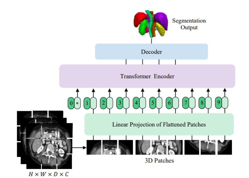
Convolutional neural networks have been the dominant machine learning architecture for computer vision since the introduction of AlexNet in 2012. Recently, inspired by the evolution of Transformers in natural language processing, attention mechanisms have been prominently incorporated into vision models. These attention methods boost some parts of the input data while minimizing other parts so that the network can focus on small but important parts of the data. The Vision Transformer (ViT) has created a new landscape of model designs for computer vision that is completely free of convolution. ViT regards image patches as a sequence of words, and applies a Transformer encoder on top. When trained on sufficiently large datasets, ViT demonstrates compelling performance on image recognition.

While convolutions and attention are both sufficient for good performance, neither of them are necessary. For example, MLP-Mixer adopts a simple multi-layer perceptron (MLP) to mix image patches across all the spatial locations, resulting in an all-MLP architecture. It is a competitive alternative to existing state-of-the-art vision models in terms of the trade-off between accuracy and computation required for training and inference. However, both ViT and the MLP models struggle to scale to higher input resolution because the computational complexity increases quadratically with respect to the image size.

Today we present a new multi-axis approach that is simple and effective, improves on the original ViT and MLP models, can better adapt to high-resolution, dense prediction tasks, and can naturally adapt to different input sizes with high flexibility and low complexity. Based on this approach, we have built two backbone models for high-level and low-level vision tasks. We describe the first in “MaxViT: Multi-Axis Vision Transformer”, to be presented in ECCV 2022, and show it significantly improves the state of the art for high-level tasks, such as image classification, object detection, segmentation, quality assessment, and generation. The second, presented in “MAXIM: Multi-Axis MLP for Image Processing” at CVPR 2022, is based on a UNet-like architecture and achieves competitive performance on low-level imaging tasks including denoising, deblurring, dehazing, deraining, and low-light enhancement. To facilitate further research on efficient Transformer and MLP models, we have open-sourced the code and models for both MaxViT and MAXIM.

A demo of image deblurring using MAXIM frame by frame.

Overview
Our new approach is based on multi-axis attention, which decomposes the full-size attention (each pixel attends to all the pixels) used in ViT into two sparse forms — local and (sparse) global. As shown in the figure below, the multi-axis attention contains a sequential stack of block attention and grid attention. The block attention works within non-overlapping windows (small patches in intermediate feature maps) to capture local patterns, while the grid attention works on a sparsely sampled uniform grid for long-range (global) interactions. The window sizes of grid and block attentions can be fully controlled as hyperparameters to ensure a linear computational complexity to the input size.

The proposed multi-axis attention conducts blocked local and dilated global attention sequentially followed by a FFN, with only a linear complexity. The pixels in the same colors are attended together.

Such low-complexity attention can significantly improve its wide applicability to many vision tasks, especially for high-resolution visual predictions, demonstrating greater generality than the original attention used in ViT. We build two backbone instantiations out of this multi-axis attention approach – MaxViT and MAXIM, for high-level and low-level tasks, respectively.

MaxViT
In MaxViT, we first build a single MaxViT block (shown below) by concatenating MBConv (proposed by EfficientNet, V2) with the multi-axis attention. This single block can encode local and global visual information regardless of input resolution. We then simply stack repeated blocks composed of attention and convolutions in a hierarchical architecture (similar to ResNet, CoAtNet), yielding our homogenous MaxViT architecture. Notably, MaxViT is distinguished from previous hierarchical approaches as it can “see” globally throughout the entire network, even in earlier, high-resolution stages, demonstrating stronger model capacity on various tasks.

The meta-architecture of MaxViT.

MAXIM
Our second backbone, MAXIM, is a generic UNet-like architecture tailored for low-level image-to-image prediction tasks. MAXIM explores parallel designs of the local and global approaches using the gated multi-layer perceptron (gMLP) network (patching-mixing MLP with a gating mechanism). Another contribution of MAXIM is the cross-gating block that can be used to apply interactions between two different input signals. This block can serve as an efficient alternative to the cross-attention module as it only employs the cheap gated MLP operators to interact with various inputs without relying on the computationally heavy cross-attention. Moreover, all the proposed components including the gated MLP and cross-gating blocks in MAXIM enjoy linear complexity to image size, making it even more efficient when processing high-resolution pictures.

Results
We demonstrate the effectiveness of MaxViT on a broad range of vision tasks. On image classification, MaxViT achieves state-of-the-art results under various settings: with only ImageNet-1K training, MaxViT attains 86.5% top-1 accuracy; with ImageNet-21K (14M images, 21k classes) pre-training, MaxViT achieves 88.7% top-1 accuracy; and with JFT (300M images, 18k classes) pre-training, our largest model MaxViT-XL achieves a high accuracy of 89.5% with 475M parameters.

Performance comparison of MaxViT with state-of-the-art models on ImageNet-1K. Top: Accuracy vs. FLOPs performance scaling with 224x224 image resolution. Bottom: Accuracy vs. parameters scaling curve under ImageNet-1K fine-tuning setting.

For downstream tasks, MaxViT as a backbone delivers favorable performance on a broad spectrum of tasks. For object detection and segmentation on the COCO dataset, the MaxViT backbone achieves 53.4 AP, outperforming other base-level models while requiring only about 60% the computational cost. For image aesthetics assessment, the MaxViT model advances the state-of-the-art MUSIQ model by 3.5% in terms of linear correlation with human opinion scores. The standalone MaxViT building block also demonstrates effective performance on image generation, achieving better FID and IS scores on the ImageNet-1K unconditional generation task with a significantly lower number of parameters than the state-of-the-art model, HiT.

The UNet-like MAXIM backbone, customized for image processing tasks, has also demonstrated state-of-the-art results on 15 out of 20 tested datasets, including denoising, deblurring, deraining, dehazing, and low-light enhancement, while requiring fewer or comparable number of parameters and FLOPs than competitive models. Images restored by MAXIM show more recovered details with less visual artifacts.

Visual results of MAXIM for image deblurring, deraining, and low-light enhancement.

Summary
Recent works in the last two or so years have shown that ConvNets and Vision Transformers can achieve similar performance. Our work presents a unified design that takes advantage of the best of both worlds — efficient convolution and sparse attention — and demonstrates that a model built on top, namely MaxViT, can achieve state-of-the-art performance on a variety of vision tasks. More importantly, MaxViT scales well to very large data sizes. We also show that an alternative multi-axis design using MLP operators, MAXIM, achieves state-of-the-art performance on a broad range of low-level vision tasks.

Even though we present our models in the context of vision tasks, the proposed multi-axis approach can easily extend to language modeling to capture both local and global dependencies in linear time. Motivated by the work here, we expect that it is worthwhile to study other forms of sparse attention in higher-dimensional or multimodal signals such as videos, point clouds, and vision-language models.

We have open-sourced the code and models of MAXIM and MaxViT to facilitate future research on efficient attention and MLP models.

Acknowledgments
We would like to thank our co-authors: Hossein Talebi, Han Zhang, Feng Yang, Peyman Milanfar, and Alan Bovik. We would also like to acknowledge the valuable discussion and support from Xianzhi Du, Long Zhao, Wuyang Chen, Hanxiao Liu, Zihang Dai, Anurag Arnab, Sungjoon Choi, Junjie Ke, Mauricio Delbracio, Irene Zhu, Innfarn Yoo, Huiwen Chang, and Ce Liu.

Source: Google AI Blog

Google Dev Library Letters : 13th Issue

Posted by Garima Mehra, Program Manager

Welcome to the 13th Issue: ‘Google Dev Library letters’ is a technology newsletter curated to bring you some of the best projects developed with Google tech and submitted to the Google Dev Library platform. We are back with another boost of inspiration for your next project!

Hero Content of the month

Check out shortlisted content from the Google technologies of your choice.

Android

Contact Store API by Alex Styl

Contact Store is a modern API that makes access to contacts on Android devices simple to use. It solves for the most frequent use cases and makes developing enjoyable.

Custom Progress Indicator by Samson Achiaga

CustomProgressIndicator library is a simple, customizable progress indicator that gives android applications a nice feel. It saves developers time by creating a unique, customizable loading view.

Flutter

Numbers by Bulent Bariskilic

Discover an app designed to show facts about numbers using the http://numbersapi.com API. The project has been written solely in Dart Language.

Cupertino Icons Gallery by Cephas Brian

Get access to over 1,335 icons in one centralized place - the Cupertino Icons Gallery is an open source, cross-platform space to find all the icons used in Flutter.

Machine Learning

MLOps System with AutoML and Pipeline in Vertex AI by Chansung Park

Learn how to build a system by considering two MLOps scenarios - if the model needs to be replaced later and if the model itself has to evolve with the data.

Probing Vision Transformers by Sayak Paul & Aritra Roy

Explore tools in this repository to probe into the representations learned by different families of Vision Transformers.

Google Cloud

Combining Google Apps Script with Google AppSheet by Aryan Irani

Learn how to combine Google AppScript with Google AppSheet to make automation even more powerful.

What a beautiful stream!! by Mandar Chaphalkar

Learn how to create a stream in 6 simple steps now that Google Cloud recently made Datastream CDC generally available.

Curators Corner

Meet our curators who have been working behind the scenes to bring you the best content submissions

Android

"Android development changes fast and it's great to see developers write blogs to help others learn.

It's a pleasure to be part of the Android community. I enjoy seeing the android community. I enjoy seeing the Android community flourish by collaborating with each other and sharing their learnings"

Andres Sandoval

Sr. Strategist, Google

Machine Learning

"We are loving the TensorFlow.js submissions we have seen so far, and have no doubt future ones will continue to push the boundaries of what's possible in this space, and because it is web powered anyone anywhere can try the demos typically with the click of a link!"

Jason Mayes

Web ML Developer Relations Lead, Google

Liked what you read? Checkout the latest projects and community-authored content by visiting our home page or subscribing to our newsletter.

Source: Google Developers Blog

High-Definition Segmentation in Google Meet

Posted by Tingbo Hou and Juhyun Lee, Software Engineers, Google

In recent years video conferencing has played an increasingly important role in both work and personal communication for many users. Over the past two years, we have enhanced this experience in Google Meet by introducing privacy-preserving machine learning (ML) powered background features, also known as “virtual green screen”, which allows users to blur their backgrounds or replace them with other images. What is unique about this solution is that it runs directly in the browser without the need to install additional software.

So far, these ML-powered features have relied on CPU inference made possible by leveraging neural network sparsity, a common solution that works across devices, from entry level computers to high-end workstations. This enables our features to reach the widest audience. However, mid-tier and high-end devices often have powerful GPUs that remain untapped for ML inference, and existing functionality allows web browsers to access GPUs via shaders (WebGL).

With the latest update to Google Meet, we are now harnessing the power of GPUs to significantly improve the fidelity and performance of these background effects. As we detail in “Efficient Heterogeneous Video Segmentation at the Edge”, these advances are powered by two major components: 1) a novel real-time video segmentation model and 2) a new, highly efficient approach for in-browser ML acceleration using WebGL. We leverage this capability to develop fast ML inference via fragment shaders. This combination results in substantial gains in accuracy and latency, leading to crisper foreground boundaries.

CPU segmentation vs. HD segmentation in Meet.

Moving Towards Higher Quality Video Segmentation Models
To predict finer details, our new segmentation model now operates on high definition (HD) input images, rather than lower-resolution images, effectively doubling the resolution over the previous model. To accommodate this, the model must be of higher capacity to extract features with sufficient detail. Roughly speaking, doubling the input resolution quadruples the computation cost during inference.

Inference of high-resolution models using the CPU is not feasible for many devices. The CPU may have a few high-performance cores that enable it to execute arbitrary complex code efficiently, but it is limited in its ability for the parallel computation required for HD segmentation. In contrast, GPUs have many, relatively low-performance cores coupled with a wide memory interface, making them uniquely suitable for high-resolution convolutional models. Therefore, for mid-tier and high-end devices, we adopt a significantly faster pure GPU pipeline, which is integrated using WebGL.

This change inspired us to revisit some of the prior design decisions for the model architecture.

Backbone: We compared several widely-used backbones for on-device networks and found EfficientNet-Lite to be a better fit for the GPU because it removes the squeeze-and-excitation block, a component that is inefficient on WebGL (more below).
Decoder: We switched to a multi-layer perceptron (MLP) decoder consisting of 1x1 convolutions instead of using simple bilinear upsampling or the more expensive squeeze-and-excitation blocks. MLP has been successfully adopted in other segmentation architectures, like DeepLab and PointRend, and is efficient to compute on both CPU and GPU.
Model size: With our new WebGL inference and the GPU-friendly model architecture, we were able to afford a larger model without sacrificing the real-time frame rate necessary for smooth video segmentation. We explored the width and the depth parameters using a neural architecture search.

HD segmentation model architecture.

In aggregate, these changes substantially improve the mean Intersection over Union (IoU) metric by 3%, resulting in less uncertainty and crisper boundaries around hair and fingers.

We have also released the accompanying model card for this segmentation model, which details our fairness evaluations. Our analysis shows that the model is consistent in its performance across the various regions, skin-tones, and genders, with only small deviations in IoU metrics.

Model	Resolution	Inference	IoU	Latency (ms)
CPU segmenter	256×144	Wasm SIMD	94.0%	8.7
GPU segmenter	512×288	WebGL	96.9%	4.3

Comparison of the previous segmentation model vs. the new HD segmentation model on a Macbook Pro (2018).

Accelerating Web ML with WebGL
One common challenge for web-based inference is that web technologies can incur a performance penalty when compared to apps running natively on-device. For GPUs, this penalty is substantial, only achieving around 25% of native OpenGL performance. This is because WebGL, the current GPU standard for Web-based inference, was primarily designed for image rendering, not arbitrary ML workloads. In particular, WebGL does not include compute shaders, which allow for general purpose computation and enable ML workloads in mobile and native apps.

To overcome this challenge, we accelerated low-level neural network kernels with fragment shaders that typically compute the output properties of a pixel like color and depth, and then applied novel optimizations inspired by the graphics community. As ML workloads on GPUs are often bound by memory bandwidth rather than compute, we focused on rendering techniques that would improve the memory access, such as Multiple Render Targets (MRT).

MRT is a feature in modern GPUs that allows rendering images to multiple output textures (OpenGL objects that represent images) at once. While MRT was originally designed to support advanced graphics rendering such as deferred shading, we found that we could leverage this feature to drastically reduce the memory bandwidth usage of our fragment shader implementations for critical operations, like convolutions and fully connected layers. We do so by treating intermediate tensors as multiple OpenGL textures.

In the figure below, we show an example of intermediate tensors having four underlying GL textures each. With MRT, the number of GPU threads, and thus effectively the number of memory requests for weights, is reduced by a factor of four and saves memory bandwidth usage. Although this introduces considerable complexities in the code, it helps us reach over 90% of native OpenGL performance, closing the gap with native applications.

Left: A classic implementation of Conv2D with 1-to-1 correspondence of tensor and an OpenGL texture. Red, yellow, green, and blue boxes denote different locations in a single texture each for intermediate tensor A and B. Right: Our implementation of Conv2D with MRT where intermediate tensors A and B are realized with a set of 4 GL textures each, depicted as red, yellow, green, and blue boxes. Note that this reduces the request count for weights by 4x.

Conclusion
We have made rapid strides in improving the quality of real-time segmentation models by leveraging the GPU on mid-tier and high-end devices for use with Google Meet. We look forward to the possibilities that will be enabled by upcoming technologies like WebGPU, which bring compute shaders to the web. Beyond GPU inference, we're also working on improving the segmentation quality for lower powered devices with quantized inference via XNNPACK WebAssembly.

Acknowledgements
Special thanks to those on the Meet team and others who worked on this project, in particular Sebastian Jansson, Sami Kalliomäki, Rikard Lundmark, Stephan Reiter, Fabian Bergmark, Ben Wagner, Stefan Holmer, Dan Gunnarsson, Stéphane Hulaud, and to all our team members who made this possible: Siargey Pisarchyk, Raman Sarokin, Artsiom Ablavatski, Jamie Lin, Tyler Mullen, Gregory Karpiak, Andrei Kulik, Karthik Raveendran, Trent Tolley, and Matthias Grundmann.

Source: Google AI Blog

Towards Helpful Robots: Grounding Language in Robotic Affordances

Posted by Brian Ichter and Karol Hausman, Research Scientists, Google Research, Brain Team

Over the last several years, we have seen significant progress in applying machine learning to robotics. However, robotic systems today are capable of executing only very short, hard-coded commands, such as “Pick up an apple,” because they tend to perform best with clear tasks and rewards. They struggle with learning to perform long-horizon tasks and reasoning about abstract goals, such as a user prompt like “I just worked out, can you get me a healthy snack?”

Meanwhile, recent progress in training language models (LMs) has led to systems that can perform a wide range of language understanding and generation tasks with impressive results. However, these language models are inherently not grounded in the physical world due to the nature of their training process: a language model generally does not interact with its environment nor observe the outcome of its responses. This can result in it generating instructions that may be illogical, impractical or unsafe for a robot to complete in a physical context. For example, when prompted with “I spilled my drink, can you help?” the language model GPT-3 responds with “You could try using a vacuum cleaner,” a suggestion that may be unsafe or impossible for the robot to execute. When asking the FLAN language model the same question, it apologizes for the spill with "I'm sorry, I didn't mean to spill it,” which is not a very useful response. Therefore, we asked ourselves, is there an effective way to combine advanced language models with robot learning algorithms to leverage the benefits of both?

In “Do As I Can, Not As I Say: Grounding Language in Robotic Affordances”, we present a novel approach, developed in partnership with Everyday Robots, that leverages advanced language model knowledge to enable a physical agent, such as a robot, to follow high-level textual instructions for physically-grounded tasks, while grounding the language model in tasks that are feasible within a specific real-world context. We evaluate our method, which we call PaLM-SayCan, by placing robots in a real kitchen setting and giving them tasks expressed in natural language. We observe highly interpretable results for temporally-extended complex and abstract tasks, like “I just worked out, please bring me a snack and a drink to recover.” Specifically, we demonstrate that grounding the language model in the real world nearly halves errors over non-grounded baselines. We are also excited to release a robot simulation setup where the research community can test this approach.

With PaLM-SayCan, the robot acts as the language model’s “hands and eyes,” while the language model supplies high-level semantic knowledge about the task.

A Dialog Between User and Robot, Facilitated by the Language Model
Our approach uses the knowledge contained in language models (Say) to determine and score actions that are useful towards high-level instructions. It also uses an affordance function (Can) that enables real-world-grounding and determines which actions are possible to execute in a given environment. Using the the PaLM language model, we call this PaLM-SayCan.

Our approach selects skills based on what the language model scores as useful to the high level instruction and what the affordance model scores as possible.

Our system can be seen as a dialog between the user and robot, facilitated by the language model. The user starts by giving an instruction that the language model turns into a sequence of steps for the robot to execute. This sequence is filtered using the robot’s skillset to determine the most feasible plan given its current state and environment. The model determines the probability of a specific skill successfully making progress toward completing the instruction by multiplying two probabilities: (1) task-grounding (i.e., a skill language description) and (2) world-grounding (i.e., skill feasibility in the current state).

There are additional benefits of our approach in terms of its safety and interpretability. First, by allowing the LM to score different options rather than generate the most likely output, we effectively constrain the LM to only output one of the pre-selected responses. In addition, the user can easily understand the decision making process by looking at the separate language and affordance scores, rather than a single output.

PaLM-SayCan is also interpretable: at each step, we can see the top options it considers based on their language score (blue), affordance score (red), and combined score (green).

Training Policies and Value Functions
Each skill in the agent’s skillset is defined as a policy with a short language description (e.g., “pick up the can”), represented as embeddings, and an affordance function that indicates the probability of completing the skill from the robot’s current state. To learn the affordance functions, we use sparse reward functions set to 1.0 for a successful execution, and 0.0 otherwise.

We use image-based behavioral cloning (BC) to train the language-conditioned policies and temporal-difference-based (TD) reinforcement learning (RL) to train the value functions. To train the policies, we collected data from 68,000 demos performed by 10 robots over 11 months and added 12,000 successful episodes, filtered from a set of autonomous episodes of learned policies. We then learned the language conditioned value functions using MT-Opt in the Everyday Robots simulator. The simulator complements our real robot fleet with a simulated version of the skills and environment, which is transformed using RetinaGAN to reduce the simulation-to-real gap. We bootstrapped simulation policies’ performance by using demonstrations to provide initial successes, and then continuously improved RL performance with online data collection in simulation.

Given a high-level instruction, our approach combines the probabilities from the language model with the probabilities from the value function (VF) to select the next skill to perform. This process is repeated until the high-level instruction is successfully completed.

Performance on Temporally-Extended, Complex, and Abstract Instructions
To test our approach, we use robots from Everyday Robots paired with PaLM. We place the robots in a kitchen environment containing common objects and evaluate them on 101 instructions to test their performance across various robot and environment states, instruction language complexity and time horizon. Specifically, these instructions were designed to showcase the ambiguity and complexity of language rather than to provide simple, imperative queries, enabling queries such as “I just worked out, how would you bring me a snack and a drink to recover?” instead of “Can you bring me water and an apple?”

We use two metrics to evaluate the system’s performance: (1) the plan success rate, indicating whether the robot chose the right skills for the instruction, and (2) the execution success rate, indicating whether it performed the instruction successfully. We compare two language models, PaLM and FLAN (a smaller language model fine-tuned on instruction answering) with and without the affordance grounding as well as the underlying policies running directly with natural language (Behavioral Cloning in the table below). The results show that the system using PaLM with affordance grounding (PaLM-SayCan) chooses the correct sequence of skills 84% of the time and executes them successfully 74% of the time, reducing errors by 50% compared to FLAN and compared to PaLM without robotic grounding. This is particularly exciting because it represents the first time we can see how an improvement in language models translates to a similar improvement in robotics. This result indicates a potential future where robotics is able to ride the wave of progress that we have been observing in language models, bringing these subfields of research closer together.

Algorithm	Plan	Execute
PaLM-SayCan	84%	74%
PaLM	67%	-
FLAN-SayCan	70%	61%
FLAN	38%	-
Behavioral Cloning	0%	0%

PaLM-SayCan halves errors compared to PaLM without affordances and compared to FLAN over 101 tasks.

SayCan demonstrated successful planning for 84% of the 101 test instructions when combined with PaLM.

If you're interested in learning more about this project from the researchers themselves, please check out the video below:

Conclusion and Future Work
We’re excited about the progress that we’ve seen with PaLM-SayCan, an interpretable and general approach to leveraging knowledge from language models that enables a robot to follow high-level textual instructions to perform physically-grounded tasks. Our experiments on a number of real-world robotic tasks demonstrate the ability to plan and complete long-horizon, abstract, natural language instructions at a high success rate. We believe that PaLM-SayCan’s interpretability allows for safe real-world user interaction with robots. As we explore future directions for this work, we hope to better understand how information gained via the robot’s real-world experience could be leveraged to improve the language model and to what extent natural language is the right ontology for programming robots. We have open-sourced a robot simulation setup, which we hope will provide researchers with a valuable resource for future research that combines robotic learning with advanced language models. The research community can visit the project’s GitHub page and website to learn more.

Acknowledgements
We’d like to thank our coauthors Michael Ahn, Anthony Brohan, Noah Brown, Yevgen Chebotar, Omar Cortes, Byron David, Chelsea Finn, Kelly Fu, Keerthana Gopalakrishnan, Alex Herzog, Daniel Ho, Jasmine Hsu, Julian Ibarz, Alex Irpan, Eric Jang, Rosario Jauregui Ruano, Kyle Jeffrey, Sally Jesmonth, Nikhil J Joshi, Ryan Julian, Dmitry Kalashnikov, Yuheng Kuang, Kuang-Huei Lee, Sergey Levine, Yao Lu, Linda Luu, Carolina Parada, Peter Pastor, Jornell Quiambao, Kanishka Rao, Jarek Rettinghouse, Diego Reyes, Pierre Sermanet, Nicolas Sievers, Clayton Tan, Alexander Toshev, Vincent Vanhoucke, Fei Xia, Ted Xiao, Peng Xu, Sichun Xu, Mengyuan Yan, and Andy Zeng. We’d also like to thank Yunfei Bai, Matt Bennice, Maarten Bosma, Justin Boyd, Bill Byrne, Kendra Byrne, Noah Constant, Pete Florence, Laura Graesser, Rico Jonschkowski, Daniel Kappler, Hugo Larochelle, Benjamin Lee, Adrian Li, Suraj Nair, Krista Reymann, Jeff Seto, Dhruv Shah, Ian Storz, Razvan Surdulescu, and Vincent Zhao for their help and support in various aspects of the project. And we’d like to thank Tom Small for creating many of the animations in this post.

Source: Google AI Blog

Rax: Composable Learning-to-Rank Using JAX

Posted by Rolf Jagerman and Honglei Zhuang, Software Engineers, Google Research

Ranking is a core problem across a variety of domains, such as search engines, recommendation systems, or question answering. As such, researchers often utilize learning-to-rank (LTR), a set of supervised machine learning techniques that optimize for the utility of an entire list of items (rather than a single item at a time). A noticeable recent focus is on combining LTR with deep learning. Existing libraries, most notably TF-Ranking, offer researchers and practitioners the necessary tools to use LTR in their work. However, none of the existing LTR libraries work natively with JAX, a new machine learning framework that provides an extensible system of function transformations that compose: automatic differentiation, JIT-compilation to GPU/TPU devices and more.

Today, we are excited to introduce Rax, a library for LTR in the JAX ecosystem. Rax brings decades of LTR research to the JAX ecosystem, making it possible to apply JAX to a variety of ranking problems and combine ranking techniques with recent advances in deep learning built upon JAX (e.g., T5X). Rax provides state-of-the-art ranking losses, a number of standard ranking metrics, and a set of function transformations to enable ranking metric optimization. All this functionality is provided with a well-documented and easy to use API that will look and feel familiar to JAX users. Please check out our paper for more technical details.

Learning-to-Rank Using Rax
Rax is designed to solve LTR problems. To this end, Rax provides loss and metric functions that operate on batches of lists, not batches of individual data points as is common in other machine learning problems. An example of such a list is the multiple potential results from a search engine query. The figure below illustrates how tools from Rax can be used to train neural networks on ranking tasks. In this example, the green items (B, F) are very relevant, the yellow items (C, E) are somewhat relevant and the red items (A, D) are not relevant. A neural network is used to predict a relevancy score for each item, then these items are sorted by these scores to produce a ranking. A Rax ranking loss incorporates the entire list of scores to optimize the neural network, improving the overall ranking of the items. After several iterations of stochastic gradient descent, the neural network learns to score the items such that the resulting ranking is optimal: relevant items are placed at the top of the list and non-relevant items at the bottom.

Using Rax to optimize a neural network for a ranking task. The green items (B, F) are very relevant, the yellow items (C, E) are somewhat relevant and the red items (A, D) are not relevant.

Approximate Metric Optimization
The quality of a ranking is commonly evaluated using ranking metrics, e.g., the normalized discounted cumulative gain (NDCG). An important objective of LTR is to optimize a neural network so that it scores highly on ranking metrics. However, ranking metrics like NDCG can present challenges because they are often discontinuous and flat, so stochastic gradient descent cannot directly be applied to these metrics. Rax provides state-of-the-art approximation techniques that make it possible to produce differentiable surrogates to ranking metrics that permit optimization via gradient descent. The figure below illustrates the use of rax.approx_t12n, a function transformation unique to Rax, which allows for the NDCG metric to be transformed into an approximate and differentiable form.

Using an approximation technique from Rax to transform the NDCG ranking metric into a differentiable and optimizable ranking loss (approx_t12n and gumbel_t12n).

First, notice how the NDCG metric (in green) is flat and discontinuous, making it hard to optimize using stochastic gradient descent. By applying the rax.approx_t12n transformation to the metric, we obtain ApproxNDCG, an approximate metric that is now differentiable with well-defined gradients (in red). However, it potentially has many local optima — points where the loss is locally optimal, but not globally optimal — in which the training process can get stuck. When the loss encounters such a local optimum, training procedures like stochastic gradient descent will have difficulty improving the neural network further.

To overcome this, we can obtain the gumbel-version of ApproxNDCG by using the rax.gumbel_t12n transformation. This gumbel version introduces noise in the ranking scores which causes the loss to sample many different rankings that may incur a non-zero cost (in blue). This stochastic treatment may help the loss escape local optima and often is a better choice when training a neural network on a ranking metric. Rax, by design, allows the approximate and gumbel transformations to be freely used with all metrics that are offered by the library, including metrics with a top-k cutoff value, like recall or precision. In fact, it is even possible to implement your own metrics and transform them to obtain gumbel-approximate versions that permit optimization without any extra effort.

Ranking in the JAX Ecosystem
Rax is designed to integrate well in the JAX ecosystem and we prioritize interoperability with other JAX-based libraries. For example, a common workflow for researchers that use JAX is to use TensorFlow Datasets to load a dataset, Flax to build a neural network, and Optax to optimize the parameters of the network. Each of these libraries composes well with the others and the composition of these tools is what makes working with JAX both flexible and powerful. For researchers and practitioners of ranking systems, the JAX ecosystem was previously missing LTR functionality, and Rax fills this gap by providing a collection of ranking losses and metrics. We have carefully constructed Rax to function natively with standard JAX transformations such as jax.jit and jax.grad and various libraries like Flax and Optax. This means that users can freely use their favorite JAX and Rax tools together.

Ranking with T5
While giant language models such as T5 have shown great performance on natural language tasks, how to leverage ranking losses to improve their performance on ranking tasks, such as search or question answering, is under-explored. With Rax, it is possible to fully tap this potential. Rax is written as a JAX-first library, thus it is easy to integrate it with other JAX libraries. Since T5X is an implementation of T5 in the JAX ecosystem, Rax can work with it seamlessly.

To this end, we have an example that demonstrates how Rax can be used in T5X. By incorporating ranking losses and metrics, it is now possible to fine-tune T5 for ranking problems, and our results indicate that enhancing T5 with ranking losses can offer significant performance improvements. For example, on the MS-MARCO QNA v2.1 benchmark we are able to achieve a +1.2% NDCG and +1.7% MRR by fine-tuning a T5-Base model using the Rax listwise softmax cross-entropy loss instead of a pointwise sigmoid cross-entropy loss.

Fine-tuning a T5-Base model on MS-MARCO QNA v2.1 with a ranking loss (softmax, in blue) versus a non-ranking loss (pointwise sigmoid, in red).

Conclusion
Overall, Rax is a new addition to the growing ecosystem of JAX libraries. Rax is entirely open source and available to everyone at github.com/google/rax. More technical details can also be found in our paper. We encourage everyone to explore the examples included in the github repository: (1) optimizing a neural network with Flax and Optax, (2) comparing different approximate metric optimization techniques, and (3) how to integrate Rax with T5X.

Acknowledgements
Many collaborators within Google made this project possible: Xuanhui Wang, Zhen Qin, Le Yan, Rama Kumar Pasumarthi, Michael Bendersky, Marc Najork, Fernando Diaz, Ryan Doherty, Afroz Mohiuddin, and Samer Hassan.

Source: Google AI Blog

Rax: Composable Learning-to-Rank Using JAX

Posted by Rolf Jagerman and Honglei Zhuang, Software Engineers, Google Research

Using Rax to optimize a neural network for a ranking task. The green items (B, F) are very relevant, the yellow items (C, E) are somewhat relevant and the red items (A, D) are not relevant.

Using an approximation technique from Rax to transform the NDCG ranking metric into a differentiable and optimizable ranking loss (approx_t12n and gumbel_t12n).

Fine-tuning a T5-Base model on MS-MARCO QNA v2.1 with a ranking loss (softmax, in blue) versus a non-ranking loss (pointwise sigmoid, in red).

Source: Google AI Blog

Google Dev Library Letters — 12th Issue

Posted by Garima Mehra, Program Manager

‘Google Dev Library Letters’ is curated to bring you some of the latest projects developed with Google tech submitted to Google Dev Library Platform. We hope this brings you the inspiration you need for your next project!

Android

Shape your Image: Circle, Rounded Square, or Cuts at the corner in Android by Sriyank Siddhartha

Using the MDC library, shape images in just a few lines of code by using ShapeableImageView.

Foso/Ktorfit by Jens Klingenberg

HTTP client / Kotlin Symbol Processor for Kotlin Multiplatform (Js, Jvm, Android, Native, iOS) using KSP and Ktor clients inspired by Retrofit.

Continue reading →

Source: Google Developers Blog

Efficient Sequence Modeling for On-Device ML

Posted by Arun Kandoor, Software Engineer, Google Research

The increasing demand for machine learning (ML) model inference on-device (for mobile devices, tablets, etc.) is driven by the rise of compute-intensive applications, the need to keep certain data on device for privacy and security reasons, and the desire to provide services when a network connection may not be available. However, on-device inference introduces a myriad of challenges, ranging from modeling to platform support requirements. These challenges relate to how different architectures are designed to optimize memory and computation, while still trying to maintain the quality of the model. From a platform perspective, the issue is identifying operations and building on top of them in a way that can generalize well across different product use cases.

In previous research, we combined a novel technique for generating embeddings (called projection-based embeddings) with efficient architectures like QRNN (pQRNN) and proved them to be competent for a number of classification problems. Augmenting these with distillation techniques provides an additional bump in end-to-end quality. Although this is an effective approach, it is not scalable to bigger and more extensive vocabularies (i.e., all possible Unicode or word tokens that can be fed to the model). Additionally, the output from the projection operation itself doesn’t contain trainable weights to take advantage of pre-training the model.

Token-free models presented in ByT5 are a good starting point for on-device modeling that can address pre-training and scalability issues without the need to increase the size of the model. This is possible because these approaches treat text inputs as a stream of bytes (each byte has a value that ranges from 0 to 255) that can reduce the vocabulary size for the embedding tables from ~30,000 to 256. Although ByT5 presents a compelling alternative for on-device modeling, going from word-level representation to byte stream representation increases the sequence lengths linearly; with an average word length of four characters and a single character having up to four bytes, the byte sequence length increases proportionally to the word length. This can lead to a significant increase in inference latency and computational costs.

We address this problem by developing and releasing three novel byte-stream sequence models for the SeqFlowLite library (ByteQRNN, ByteTransformer and ByteFunnelTransformer), all of which can be pre-trained on unsupervised data and can be fine-tuned for specific tasks. These models leverage recent innovations introduced by Charformer, including a fast character Transformer-based model that uses a gradient-based subword tokenization (GBST) approach to operate directly at the byte level, as well as a “soft” tokenization approach, which allows us to learn token boundaries and reduce sequence lengths. In this post, we focus on ByteQRNN and demonstrate that the performance of a pre-trained ByteQRNN model is comparable to BERT, despite being 300x smaller.

Sequence Model Architecture
We leverage pQRNN, ByT5 and Charformer along with platform optimizations, such as in-training quantization (which tracks minimum and maximum float values for model activations and weights for quantizing the inference model) that reduces model sizes by one-fourth, to develop an end-to-end model called ByteQRNN (shown below). First, we use a ByteSplitter operation to split the input string into a byte stream and feed it to a smaller embedding table that has a vocabulary size of 259 (256 + 3 additional meta tokens).

The output from the embedding layer is fed to the GBST layer, which is equipped with in-training quantization and combines byte-level representations with the efficiency of subword tokenization while enabling end-to-end learning of latent subwords. We “soft” tokenize the byte stream sequences by enumerating and combining each subword block length with scores (computed with a quantized dense layer) at each strided token position (i.e., at token positions that are selected at regular intervals). Next, we downsample the byte stream to manageable sequence length and feed it to the encoder layer.

The output from the GBST layer can be downsampled to a lower sequence length for efficient encoder computation or can be used by an encoder, like Funnel Transformer, which pools the query length and reduces the self-attention computation to create the ByteFunnelTransformer model. The encoder in the end-to-end model can be replaced with any other encoder layer, such as the Transformer from the SeqFlowLite library, to create a ByteTransformer model.

A diagram of a generic end-to-end sequence model using byte stream input. The ByteQRNN model uses a QRNN encoder from the SeqFlowLite library.

In addition to the input embeddings (i.e., the output from the embedding layer described above), we go a step further to build an effective sequence-to-sequence (seq2seq) model. We do so by taking ByteQRNN and adding a Transformer-based decoder model along with a quantized beam search (or tree exploration) to go with it. The quantized beam search module reduces the inference latency when generating decoder outputs by computing the most likely beams (i.e., possible output sequences) using the logarithmic sum of previous and current probabilities and returns the resulting top beams. Here the system uses a more efficient 8-bit integer (uint8) format, compared to a typical single-precision floating-point format (float32) model.

The decoder Transformer model uses a merged attention sublayer (MAtt) to reduce the complexity of the decoder self-attention from quadratic to linear, thereby lowering the end-to-end latency. For each decoding step, MAtt uses a fixed-size cache for decoder self-attention compared to the increasing cache size of a traditional transformer decoder. The following figure illustrates how the beam search module interacts with the decoder layer to generate output tokens on-device using an edge device (e.g., mobile phones, tablets, etc.).

A comparison of cloud server decoding and on-device (edge device) implementation. Left: Cloud server beam search employs a Transformer-based decoder model with quadratic time self-attention in float32, which has an increasing cache size for each decoding step. Right: The edge device implementation employs a quantized beam search module along with a fixed-size cache and a linear time self-attention computation.

Evaluation
After developing ByteQRNN, we evaluate its performance on the civil_comments dataset using the area under the curve (AUC) metric and compare it to a pre-trained ByteQRNN and BERT (shown below). We demonstrate that the fine-tuned ByteQRNN improves the overall quality and brings its performance closer to the BERT models, despite being 300x smaller. Since SeqFlowLite models support in-training quantization that reduces model sizes by one-fourth, the resulting models scale well to low-compute devices. We chose multilingual data sources that related to the task for pre-training both BERT and byte stream models to achieve the best possible performance.

Comparison of ByteQRNN with fine-tuned ByteQRNN and BERT on the civil_comments dataset.

Conclusion
Following up on our previous work with pQRNN, we evaluate byte stream models for on-device use to enable pre-training and thereby improve model performance for on-device deployment. We present an evaluation for ByteQRNN with and without pre-training and demonstrate that the performance of the pre-trained ByteQRNN is comparable to BERT, despite being 300x smaller. In addition to ByteQRNN, we are also releasing ByteTransformer and ByteFunnelTransformer, two models which use different encoders, along with the merged attention decoder model and the beam search driver to run the inference through the SeqFlowLite library. We hope these models will provide researchers and product developers with valuable resources for future on-device deployments.

Acknowledgements
We would like to thank Khoa Trinh, Jeongwoo Ko, Peter Young and Yicheng Fan for helping with open-sourcing and evaluating the model. Thanks to Prabhu Kaliamoorthi for all the brainstorming and ideation. Thanks to Vinh Tran, Jai Gupta and Yi Tay for their help with pre-training byte stream models. Thanks to Ruoxin Sang, Haoyu Zhang, Ce Zheng, Chuanhao Zhuge and Jieying Luo for helping with the TPU training. Many thanks to Erik Vee, Ravi Kumar and the Learn2Compress leadership for sponsoring the project and their support and encouragement. Finally, we would like to thank Tom Small for the animated figure used in this post.

Source: Google AI Blog

Machine Learning Communities: Q2 ‘22 highlights and achievements

Posted by Nari Yoon, Hee Jung, DevRel Community Manager / Soonson Kwon, DevRel Program Manager

Let’s explore highlights and accomplishments of vast Google Machine Learning communities over the second quarter of the year! We are enthusiastic and grateful about all the activities by the global network of ML communities. Here are the highlights!

TensorFlow/Keras

TFUG Agadir hosted #MLReady phase as a part of #30DaysOfML. #MLReady aimed to prepare the attendees with the knowledge required to understand the different types of problems which deep learning can solve, and helped attendees be prepared for the TensorFlow Certificate.

TFUG Taipei hosted the basic Python and TensorFlow courses named From Python to TensorFlow. The aim of these events is to help everyone learn about the basics of Python and TensorFlow, including TensorFlow Hub, TensorFlow API. The event videos are shared every week via Youtube playlist.

TFUG New York hosted Introduction to Neural Radiance Fields for TensorFlow users. The talk included Volume Rendering, 3D view synthesis, and links to a minimal implementation of NeRF using Keras and TensorFlow. In the event, ML GDE Aritra Roy Gosthipaty (India) had a talk focusing on breaking the concepts of the academic paper, NeRF: Representing Scenes as Neural Radiance Fields for View Synthesis into simpler and more ingestible snippets.

TFUG Turkey, GDG Edirne and GDG Mersin organized a TensorFlow Bootcamp 22 and ML GDE M. Yusuf Sarıgöz (Turkey) participated as a speaker, TensorFlow Ecosystem: Get most out of auxiliary packages. Yusuf demonstrated the inner workings of TensorFlow, how variables, tensors and operations interact with each other, and how auxiliary packages are built upon this skeleton.

TFUG Mumbai hosted the June Meetup and 110 folks gathered. ML GDE Sayak Paul (India) and TFUG mentor Darshan Despande shared knowledge through sessions. And ML workshops for beginners went on and participants built up machine learning models without writing a single line of code.

ML GDE Hugo Zanini (Brazil) wrote Realtime SKU detection in the browser using TensorFlow.js. He shared a solution for a well-known problem in the consumer packaged goods (CPG) industry: real-time and offline SKU detection using TensorFlow.js.

ML GDE Gad Benram (Portugal) wrote Can a couple TensorFlow lines reduce overfitting? He explained how just a few lines of code can generate data augmentations and boost a model’s performance on the validation set.

ML GDE Victor Dibia (USA) wrote How to Build An Android App and Integrate Tensorflow ML Models sharing how to run machine learning models locally on Android mobile devices, How to Implement Gradient Explanations for a HuggingFace Text Classification Model (Tensorflow 2.0) explaining in 5 steps about how to verify the model is focusing on the right tokens to classify text. He also wrote how to finetune a HuggingFace model for text classification, using Tensorflow 2.0.

ML GDE Karthic Rao (India) released a new series ML for JS developers with TFJS. This series is a combination of short portrait and long landscape videos. You can learn how to build a toxic word detector using TensorFlow.js.

ML GDE Sayak Paul (India) implemented the DeiT family of ViT models, ported the pre-trained params into the implementation, and provided code for off-the-shelf inference, fine-tuning, visualizing attention rollout plots, distilling ViT models through attention. (code | pretrained model | tutorial)

ML GDE Sayak Paul (India) and ML GDE Aritra Roy Gosthipaty (India) inspected various phenomena of a Vision Transformer, shared insights from various relevant works done in the area, and provided concise implementations that are compatible with Keras models. They provide tools to probe into the representations learned by different families of Vision Transformers. (tutorial | code)

JAX/Flax

ML GDE Aakash Nain (India) had a special talk, Introduction to JAX for ML GDEs, TFUG organizers and ML community network organizers. He covered the fundamentals of JAX/Flax so that more and more people try out JAX in the near future.

ML GDE Seunghyun Lee (Korea) started a project, Training and Lightweighting Cookbook in JAX/FLAX. This project attempts to build a neural network training and lightweighting cookbook including three kinds of lightweighting solutions, i.e., knowledge distillation, filter pruning, and quantization.

ML GDE Yucheng Wang (China) wrote History and features of JAX and explained the difference between JAX and Tensorflow.

ML GDE Martin Andrews (Singapore) shared a video, Practical JAX : Using Hugging Face BERT on TPUs. He reviewed the Hugging Face BERT code, written in JAX/Flax, being fine-tuned on Google’s Colab using Google TPUs. (Notebook for the video)

ML GDE Soumik Rakshit (India) wrote Implementing NeRF in JAX. He attempts to create a minimal implementation of 3D volumetric rendering of scenes represented by Neural Radiance Fields.

Kaggle

ML GDEs’ Kaggle notebooks were announced as the winner of Google OSS Expert Prize on Kaggle: Sayak Paul and Aritra Roy Gosthipaty’s Masked Image Modeling with Autoencoders in March; Sayak Paul’s Distilling Vision Transformers in April; Sayak Paul & Aritra Roy Gosthipaty’s Investigating Vision Transformer Representations; Soumik Rakshit’s Tensorflow Implementation of Zero-Reference Deep Curve Estimation in May and Aakash Nain’s The Definitive Guide to Augmentation in TensorFlow and JAX in June.

ML GDE Luca Massaron (Italy) published The Kaggle Book with Konrad Banachewicz. This book details competition analysis, sample code, end-to-end pipelines, best practices, and tips & tricks. And in the online event, Luca and the co-author talked about how to compete on Kaggle.

ML GDE Ertuğrul Demir (Turkey) wrote Kaggle Handbook: Fundamentals to Survive a Kaggle Shake-up covering bias-variance tradeoff, validation set, and cross validation approach. In the second post of the series, he showed more techniques using analogies and case studies.

TFUG Chennai hosted ML Study Jam with Kaggle and created study groups for the interested participants. More than 60% of members were active during the whole program and many of them shared their completion certificates.

TFUG Mysuru organizer Usha Rengaraju shared a Kaggle notebook which contains the implementation of the research paper: UNETR - Transformers for 3D Biomedical Image Segmentation. The model automatically segments the stomach and intestines on MRI scans.

TFX

ML GDE Sayak Paul (India) and ML GDE Chansung Park (Korea) shared how to deploy a deep learning model with Docker, Kubernetes, and Github actions, with two promising ways - FastAPI (for REST) and TF Serving (for gRPC).

ML GDE Ukjae Jeong (Korea) and ML Engineers at Karrot Market, a mobile commerce unicorn with 23M users, wrote Why Karrot Uses TFX, and How to Improve Productivity on ML Pipeline Development.

ML GDE Jun Jiang (China) had a talk introducing the concept of MLOps, the production-level end-to-end solutions of Google & TensorFlow, and how to use TFX to build the search and recommendation system & scientific research platform for large-scale machine learning training.

ML GDE Piero Esposito (Brazil) wrote Building Deep Learning Pipelines with Tensorflow Extended. He showed how to get started with TFX locally and how to move a TFX pipeline from local environment to Vertex AI; and provided code samples to adapt and get started with TFX.

TFUG São Paulo (Brazil) had a series of online webinars on TensorFlow and TFX. In the TFX session, they focused on how to put the models into production. They talked about the data structures in TFX and implementation of the first pipeline in TFX: ingesting and validating data.

TFUG Stockholm hosted MLOps, TensorFlow in Production, and TFX covering why, what and how you can effectively leverage MLOps best practices to scale ML efforts and had a look at how TFX can be used for designing and deploying ML pipelines.

Cloud AI

ML GDE Chansung Park (Korea) wrote MLOps System with AutoML and Pipeline in Vertex AI on GCP official blog. He showed how Google Cloud Storage and Google Cloud Functions can help manage data and handle events in the MLOps system.

He also shared the Github repository, Continuous Adaptation with VertexAI's AutoML and Pipeline. This contains two notebooks to demonstrate how to automate to produce a new AutoML model when the new dataset comes in.

TFUG Northwest (Portland) hosted The State and Future of AI + ML/MLOps/VertexAI lab walkthrough. In this event, ML GDE Al Kari (USA) outlined the technology landscape of AI, ML, MLOps and frameworks. Googler Andrew Ferlitsch had a talk about Google Cloud AI’s definition of the 8 stages of MLOps for enterprise scale production and how Vertex AI fits into each stage. And MLOps engineer Chris Thompson covered how easy it is to deploy a model using the Vertex AI tools.

Research

ML GDE Qinghua Duan (China) released a video which introduces Google’s latest 540 billion parameter model. He introduced the paper PaLM, and described the basic training process and innovations.

ML GDE Rumei LI (China) wrote blog postings reviewing papers, DeepMind's Flamingo and Google's PaLM.

Source: Google Developers Blog

Simplified Transfer Learning for Chest Radiography Model Development

Posted by Akib Uddin, Product Manager and Andrew Sellergren, Software Engineer, Google Health

Every year, nearly a billion chest X-ray (CXR) images are taken globally to aid in the detection and management of health conditions ranging from collapsed lungs to infectious diseases. Generally, CXRs are cheaper and more accessible than other forms of medical imaging. However, existing challenges continue to impede the optimal use of CXRs. For example, in some areas, trained radiologists that can accurately interpret CXR images are in short supply. In addition, interpretation variability between experts, workflow differences between institutions, and the presence of rare conditions familiar only to subspecialists all contribute to making high-quality CXR interpretation a challenge.

Recent research has leveraged machine learning (ML) to explore potential solutions for some of these challenges. There is significant interest and effort devoted to building deep learning models that detect abnormalities in CXRs and improve access, accuracy, and efficiency to identify diseases and conditions that affect the heart and lungs. However, building robust CXR models requires large labeled training datasets, which can be prohibitively expensive and time-consuming to create. In some cases, such as working with underrepresented populations or studying rare medical conditions, only limited data are available. Additionally, CXR images vary in quality across populations, geographies, and institutions, making it difficult to build robust models that perform well globally.

In “Simplified Transfer Learning for Chest Radiography Models Using Less Data”, published in the journal Radiology, we describe how Google Health utilizes advanced ML methods to generate pre-trained “CXR networks” that can convert CXR images to embeddings (i.e., information-rich numerical vectors) to enable the development of CXR models using less data and fewer computational resources. We demonstrate that even with less data and compute, this approach has enabled performance comparable to state-of-the-art deep learning models across various prediction tasks. We are also excited to announce the release of CXR Foundation, a tool that utilizes our CXR-specific network to enable developers to create custom embeddings for their CXR images. We believe this work will help accelerate the development of CXR models, aiding in disease detection and contributing to more equitable health access throughout the world.

Developing a Chest X-ray Network
A common approach to building medical ML models is to pre-train a model on a generic task using non-medical datasets and then refine the model on a target medical task. This process of transfer learning may improve the target task performance or at least speed up convergence by applying the understanding of natural images to medical images. However, transfer learning may still require large labeled medical datasets for the refinement step.

Expanding on this standard approach, our system supports modeling CXR-specific tasks through a three-step model training setup composed of (1) generic image pre-training similar to traditional transfer learning, (2) CXR-specific pre-training, and (3) task-specific training. The first and third steps are common in ML: first pre-training on a large dataset and labels that are not specific to the desired task, and then fine-tuning on the task of interest.

We built a CXR-specific image classifier that employs supervised contrastive learning (SupCon). SupCon pulls together representations of images that have the same label (e.g., abnormal) and pushes apart representations of images that have a different label (e.g., one normal image and one abnormal image). We pre-trained this model on de-identified CXR datasets of over 800,000 images generated in partnership with Northwestern Medicine and Apollo Hospitals in the US and India, respectively. We then leveraged noisy abnormality labels from natural language processing of radiology reports to build our “CXR-specific” network.

This network creates embeddings (i.e., information-rich numerical vectors that can be used to distinguish classes from each other) that can more easily train models for specific medical prediction tasks, such as image finding (e.g., airspace opacity), clinical condition (e.g., tuberculosis), or patient outcome (e.g., hospitalization). For example, the CXR network can generate embeddings for every image in a given CXR dataset. For these images, the generated embeddings and the labels for the desired target task (such as tuberculosis) are used as examples to train a small ML model.

Left: Training a CXR model for a given task generally requires a large number of labeled images and a significant amount of computational resources to create a foundation of neural network layers. Right: With the CXR network and tool providing this foundation, each new task requires only a fraction of the labeled images, computational resources, and neural network parameters compared to rebuilding the entire network from scratch.

Effects of CXR Pre-training
We visualized these embedding layers at each step of the process using airspace opacity as an example (see the figure below). Before SupCon-based pre-training, there was poor separation of normal and abnormal CXR embeddings. After SupCon-based pre-training, the positive examples were grouped more closely together, and the negative examples more closely together as well, indicating that the model had identified that images from each category resembled themselves.

Visualizations of the t-distributed stochastic neighbor embedding for generic vs. CXR-specific network embeddings. Embeddings are information-rich numerical vectors that alone can distinguish classes from each other, in this case, airspace opacity positive vs. negative.

Our research suggests that adding the second stage of pre-training enables high-quality models to be trained with up to 600-fold less data in comparison to traditional transfer learning approaches that leverage pre-trained models on generic, non-medical datasets. We found this to be true regardless of model architecture (e.g., ResNet or EfficientNet) or dataset used for natural image pre-training (e.g., ImageNet or JFT-300M). With this approach, researchers and developers can significantly reduce dataset size requirements.

Top: In a deep learning model, the neural network contains multiple layers of artificial neurons, with the first layer taking the CXR image as input, intermediate layers doing additional computation, and the final layer making the classification (e.g., airspace opacity: present vs. absent). The embedding layer is usually one of the last layers. Bottom left: The traditional transfer learning approach involves a two-step training setup where a generic pre-trained network is optimized directly on a prediction task of interest. Our proposed three-step training setup generates a CXR network using a SupCon ML technique (step 2) before optimization for prediction tasks of interest (step 3). Bottom right: Using the embeddings involves either training smaller models (the first two strategies) or fine-tuning the whole network if there are sufficient data (strategy 3).

Results
After training the initial model, we measured performance using the area under the curve (AUC) metric with both linear and non-linear models applied to CXR embeddings; and a non-linear model produced by fine-tuning the entire network. On public datasets, such as ChestX-ray14 and CheXpert, our work substantially and consistently improved the data-accuracy tradeoff for models developed across a range of training dataset sizes and several findings. For example, when evaluating the tool’s ability to develop tuberculosis models, data efficiency gains were more striking: models trained on the embeddings of just 45 images achieved non-inferiority to radiologists in detecting tuberculosis on an external validation dataset. For both tuberculosis and severe COVID-19 outcomes, we show that non-linear classifiers trained on frozen embeddings outperformed a model that was fine-tuned on the entire dataset.

Comparing CXR-specific networks for transfer learning (red), with a baseline transfer learning approach (blue) across a variety of CXR abnormalities (top left), tuberculosis (bottom left), and COVID-19 outcomes (bottom right). This approach improves performance at the same dataset size, or reduces the dataset size required to reach the same performance. Interestingly, using the CXR network with simpler ML models that are faster to train (red) performs better than training the full network (black) at dataset sizes up to 8⁵ images.

Conclusion and Future Work
To accelerate CXR modeling efforts with low data and computational requirements, we are releasing our CXR Foundation tool, along with scripts to train linear and nonlinear classifiers. Via these embeddings, this tool will allow researchers to jump-start CXR modeling efforts using simpler transfer learning methods. This approach can be particularly useful for predictive modeling using small datasets, and for adapting CXR models when there are distribution shifts in patient populations (whether over time or across different institutions). We are excited to continue working with partners, such as Northwestern Medicine and Apollo Hospitals, to explore the impact of this technology further. By enabling researchers with limited data and compute to develop CXR models, we're hoping more developers can solve the most impactful problems for their populations.

Acknowledgements
Key contributors to this project at Google include Christina Chen, Yun Liu, Dilip Krishnan, Zaid Nabulsi, Atilla Kiraly, Arnav Agharwal, Eric Wu, Yuanzhen Li, Aaron Maschinot, Aaron Sarna, Jenny Huang, Marilyn Zhang, Charles Lau, Neeral Beladia, Daniel Tse, Krish Eswaran, and Shravya Shetty. Significant contributions and input were also made by collaborators Sreenivasa Raju Kalidindi, Mozziyar Etemadi, Florencia Garcia-Vicente, and David Melnick. For the ChestX-ray14 dataset, we thank the NIH Clinical Center for making it publicly available. The authors would also like to acknowledge many members of the Google Health Radiology and labeling software teams. Sincere appreciation also goes to the radiologists who enabled this work with their image interpretation and annotation efforts throughout the study; Jonny Wong for coordinating the imaging annotation work; Craig Mermel and Akinori Mitani for providing feedback on the manuscript; Nicole Linton and Lauren Winer for feedback on the blogpost; and Tom Small for the animation.