Tag Archives: machine learning

Dev Library Letters: 14th Issue

Posted by Garima Mehra, Program Manager

‘Google Dev Library letters’ is curated to bring you some of the best projects developed with Google tech that have been submitted to the Dev Library platform. We hope this brings you the inspiration you need for your next project!

Android

Image-compressor
by Vinod Baste

Check out Vinod’s Android Image compress library that helps reduce the size of the image by 90% without losing any of its pixels.

SealedX
by Jaewoong Eum

Learn how to auto-generate extensive sealed classes and interfaces for Android and Kotlin.

Flutter

GitHub Actions to deploy
Flutter Web to gh-pages
by Sai Rajendra Immadi

Tired of manually deploying the app every time? Or do you want to deploy your flutter web applications to gh-pages? Use this blog as your guide.

Double And Triple Dots in Flutter
by Lakshydeep Vikram

Learn the reason for using double and triple dots in flutter and where to use them.

Machine Learning

Nystromformer
by Rishit Dagli

Learn how to use the Nystrom method to approximate standard self-attention.

Google Cloud

Notification system for Cloud Run with Google Chat for CI/CD pipelines

by Ezekias Bokove

Learn how to set up a notification system for Cloud Run services.

Switch to GCP for cost savings and better performance
by Gaurav Madan

Learn why architects dealing with complex application design and who use well-known Google services should consider the Google Cloud Platform.

"The Google community includes people with diverse backgrounds. No matter what an individual circumstance is, the platform should support anyone to explore and be creative. We encourage authors to boldly consider diverse backgrounds and to be inclusive when authoring."

Vinesh Prasanna M

Customer Engineer | Google Cloud

"Authoring a good code sample is hard. The difficulty comes from the additional pieces you need to add to your respository to keep the code sample fresh and appealing to your developers."

Brett Morgan

Developer Relations Engineer | Flutter

Want to read more?

Check out the latest projects and community-authored content by visiting Google Dev Library.

Submit your projects to showcase your work and inspire developers!

Source: Google Developers Blog

AudioLM: a Language Modeling Approach to Audio Generation

Posted by Zalán Borsos, Research Software Engineer, and Neil Zeghidour, Research Scientist, Google Research

Generating realistic audio requires modeling information represented at different scales. For example, just as music builds complex musical phrases from individual notes, speech combines temporally local structures, such as phonemes or syllables, into words and sentences. Creating well-structured and coherent audio sequences at all these scales is a challenge that has been addressed by coupling audio with transcriptions that can guide the generative process, be it text transcripts for speech synthesis or MIDI representations for piano. However, this approach breaks when trying to model untranscribed aspects of audio, such as speaker characteristics necessary to help people with speech impairments recover their voice, or stylistic components of a piano performance.

In “AudioLM: a Language Modeling Approach to Audio Generation”, we propose a new framework for audio generation that learns to generate realistic speech and piano music by listening to audio only. Audio generated by AudioLM demonstrates long-term consistency (e.g., syntax in speech, melody in music) and high fidelity, outperforming previous systems and pushing the frontiers of audio generation with applications in speech synthesis or computer-assisted music. Following our AI Principles, we've also developed a model to identify synthetic audio generated by AudioLM.

From Text to Audio Language Models
In recent years, language models trained on very large text corpora have demonstrated their exceptional generative abilities, from open-ended dialogue to machine translation or even common-sense reasoning. They have further shown their capacity to model other signals than texts, such as natural images. The key intuition behind AudioLM is to leverage such advances in language modeling to generate audio without being trained on annotated data.

However, some challenges need to be addressed when moving from text language models to audio language models. First, one must cope with the fact that the data rate for audio is significantly higher, thus leading to much longer sequences — while a written sentence can be represented by a few dozen characters, its audio waveform typically contains hundreds of thousands of values. Second, there is a one-to-many relationship between text and audio. This means that the same sentence can be rendered by different speakers with different speaking styles, emotional content and recording conditions.

To overcome both challenges, AudioLM leverages two kinds of audio tokens. First, semantic tokens are extracted from w2v-BERT, a self-supervised audio model. These tokens capture both local dependencies (e.g., phonetics in speech, local melody in piano music) and global long-term structure (e.g., language syntax and semantic content in speech, harmony and rhythm in piano music), while heavily downsampling the audio signal to allow for modeling long sequences.

However, audio reconstructed from these tokens demonstrates poor fidelity. To overcome this limitation, in addition to semantic tokens, we rely on acoustic tokens produced by a SoundStream neural codec, which capture the details of the audio waveform (such as speaker characteristics or recording conditions) and allow for high-quality synthesis. Training a system to generate both semantic and acoustic tokens leads simultaneously to high audio quality and long-term consistency.

Training an Audio-Only Language Model
AudioLM is a pure audio model that is trained without any text or symbolic representation of music. AudioLM models an audio sequence hierarchically, from semantic tokens up to fine acoustic tokens, by chaining several Transformer models, one for each stage. Each stage is trained for the next token prediction based on past tokens, as one would train a text language model. The first stage performs this task on semantic tokens to model the high-level structure of the audio sequence.

In the second stage, we concatenate the entire semantic token sequence, along with the past coarse acoustic tokens, and feed both as conditioning to the coarse acoustic model, which then predicts the future tokens. This step models acoustic properties such as speaker characteristics in speech or timbre in music.

In the third stage, we process the coarse acoustic tokens with the fine acoustic model, which adds even more detail to the final audio. Finally, we feed acoustic tokens to the SoundStream decoder to reconstruct a waveform.

After training, one can condition AudioLM on a few seconds of audio, which enables it to generate consistent continuation. In order to showcase the general applicability of the AudioLM framework, we consider two tasks from different audio domains:

Speech continuation, where the model is expected to retain the speaker characteristics, prosody and recording conditions of the prompt while producing new content that is syntactically correct and semantically consistent.
Piano continuation, where the model is expected to generate piano music that is coherent with the prompt in terms of melody, harmony and rhythm.

In the video below, you can listen to examples where the model is asked to continue either speech or music and generate new content that was not seen during training. As you listen, note that everything you hear after the gray vertical line was generated by AudioLM and that the model has never seen any text or musical transcription, but rather just learned from raw audio. We release more samples on this webpage.

To validate our results, we asked human raters to listen to short audio clips and decide whether it is an original recording of human speech or a synthetic continuation generated by AudioLM. Based on the ratings collected, we observed a 51.2% success rate, which is not statistically significantly different from the 50% success rate achieved when assigning labels at random. This means that speech generated by AudioLM is hard to distinguish from real speech for the average listener.

Our work on AudioLM is for research purposes and we have no plans to release it more broadly at this time. In alignment with our AI Principles, we sought to understand and mitigate the possibility that people could misinterpret the short speech samples synthesized by AudioLM as real speech. For this purpose, we trained a classifier that can detect synthetic speech generated by AudioLM with very high accuracy (98.6%). This shows that despite being (almost) indistinguishable to some listeners, continuations generated by AudioLM are very easy to detect with a simple audio classifier. This is a crucial first step to help protect against the potential misuse of AudioLM, with future efforts potentially exploring technologies such as audio “watermarking”.

Conclusion
We introduce AudioLM, a language modeling approach to audio generation that provides both long-term coherence and high audio quality. Experiments on speech generation show not only that AudioLM can generate syntactically and semantically coherent speech without any text, but also that continuations produced by the model are almost indistinguishable from real speech by humans. Moreover, AudioLM goes well beyond speech and can model arbitrary audio signals such as piano music. This encourages the future extensions to other types of audio (e.g., multilingual speech, polyphonic music, and audio events) as well as integrating AudioLM into an encoder-decoder framework for conditioned tasks such as text-to-speech or speech-to-speech translation.

Acknowledgments
The work described here was authored by Zalán Borsos, Raphaël Marinier, Damien Vincent, Eugene Kharitonov, Olivier Pietquin, Matt Sharifi, Olivier Teboul, David Grangier, Marco Tagliasacchi and Neil Zeghidour. We are grateful for all discussions and feedback on this work that we received from our colleagues at Google.

Source: Google AI Blog

Lyra V2 – a better, faster, and more versatile speech codec

Since we open sourced the first version of Lyra on GitHub last year, we are delighted to see a vibrant community growing around it, with thousands of stars, hundreds of forks, and many comments and pull requests. There are people who fixed and formatted our code, built continuous integration for the project, and even added support for Web Assembly.

We are incredibly grateful for all these contributions, and we also heard the community's feedback, asking us to improve Lyra. Some examples of what developers wanted were to run Lyra on more platforms, develop applications in more languages; and for a model that computes faster with more bitrate options and lower latency, and better audio quality with fewer artifacts.

That's why we are now releasing Lyra V2, with a new architecture that enjoys a wider platform support, provides scalable bitrate capabilities, has better performance, and generates higher quality audio. With this release, we hope to continue to evolve with the community, and with its collective creativity, see new applications being developed and new directions emerging.

New Architecture

Lyra V2 is based on an end-to-end neural audio codec called SoundStream. The architecture has a residual vector quantizer (RVQ) sitting before and after the transmission channel, which quantizes the encoded information into a bitstream and reconstructs it on the decoder side.

The integration of RVQ into the architecture allows changing the bitrate of Lyra V2 at any time by selecting the number of quantizers to use. When more quantizers are used, higher quality audio is generated (at a cost of a higher bitrate). In Lyra V2, we support three different bitrates: 3.2 kps, 6 kbps, and 9.2 kbps. This enables developers to choose a bitrate most suitable for their network condition and quality requirements.

Lyra V2's model is exported in TensorFlow Lite, TensorFlow's lightweight cross-platform solution for mobile and embedded devices, which supports various platforms and hardware accelerations. The code is tested on Android phones and Linux, with experimental Mac and Windows support. Operation on iOS and other embedded platforms is not currently supported, although we expect it is possible with additional effort. Moreover, this paradigm opens Lyra to any future platform supported by TensorFlow Lite.

Better Performance

With the new architecture, the delay is reduced from 100 ms with the previous version to 20 ms. In this regard, Lyra V2 is comparable to the most widely used audio codec Opus for WebRTC, which has a typical delay of 26.5 ms, 46.5 ms, and 66.5 ms.

Lyra V2 also encodes and decodes five times faster than the previous version. On a Pixel 6 Pro phone, Lyra V2 takes 0.57 ms to encode and decode a 20 ms audio frame, which is 35 times faster than real time. The reduced complexity means that more phones can run Lyra V2 in real time than V1, and that the overall battery consumption is lowered.

Higher Quality

Driven by the advance of machine learning research over the years, the quality of the generated audio is also improved. Our listening tests show that the audio quality (measured in MUSHRA score, an indication of subjective quality) of Lyra V2 at 3.2 kbps, 6 kbps, and
9.2 kbps measures up to Opus at 10 kbps, 13 kbps, and 14 kbps respectively.

	Sample 1	Sample 2
Original
Opus @6kbps
LyraV1
Opus @10kbps
LyraV2 @3.2kbps
Opus @13k
LyraV2 @6kbps
Opus @14kbps
LyraV2 @9.2kbps

This makes Lyra V2 a competitive alternative to other state-of-the-art telephony codecs. While Lyra V1 already compares favorably to the Adaptive Multi-Rate (AMR-NB) codec, Lyra V2 further outperforms Enhanced Voice Services (EVS) and Adaptive Multi-Rate Wideband (AMR-WB), and is on par with Opus, all the while using only 50% - 60% of their bandwidth.

	Sample 1	Sample 2
Original
AMR-NB
LyraV1
EVS
AMR-WB
Opus @13kbps
LyraV2 @6kbps

This means more devices can be connected in bandwidth-constrained environments, or that additional information can be sent over the network to reduce voice choppiness through forward error correction and packet loss concealment.

Open Source Release

Lyra V2 continues to provide what is already in Lyra V1 (the build tools, the testing frameworks, the C++ encoding and decoding API, the signal processing toolchain, and the example Android app). Developers who have experience with the Lyra V1 API will find that the V2 API looks familiar, but with a few changes. For example, now it's possible to change bitrates during encoding (more information is available in the release notes). In addition, the model definitions and weights are included as .tflite files. As with V1, this release is a beta version and the API and bitstream are expected to change. The code for running Lyra is open sourced under the Apache license. We can’t wait to see what innovative applications people will create with the new and improved Lyra!

By Ｈengchin Yeh - Chrome

Acknowledgements

The following people helped make the open source release possible: from Chrome: Alejandro Luebs, Michael Chinen, Andrew Storus, Tom Denton, Felicia Lim, Bastiaan Kleijn, Jan Skoglund, Yaowu Xu, Jamieson Brettle, Omer Osman, Matt Frost, Jim Bankoski; and from Google Research: Neil Zeghidour, Marco Tagliasacchi

Source: Google Open Source Blog

View Synthesis with Transformers

Posted by Carlos Esteves and Ameesh Makadia, Research Scientists, Google Research

A long-standing problem in the intersection of computer vision and computer graphics, view synthesis is the task of creating new views of a scene from multiple pictures of that scene. This has received increased attention [1, 2, 3] since the introduction of neural radiance fields (NeRF). The problem is challenging because to accurately synthesize new views of a scene, a model needs to capture many types of information — its detailed 3D structure, materials, and illumination — from a small set of reference images.

In this post, we present recently published deep learning models for view synthesis. In “Light Field Neural Rendering” (LFNR), presented at CVPR 2022, we address the challenge of accurately reproducing view-dependent effects by using transformers that learn to combine reference pixel colors. Then in “Generalizable Patch-Based Neural Rendering” (GPNR), to be presented at ECCV 2022, we address the challenge of generalizing to unseen scenes by using a sequence of transformers with canonicalized positional encoding that can be trained on a set of scenes to synthesize views of new scenes. These models have some unique features. They perform image-based rendering, combining colors and features from the reference images to render novel views. They are purely transformer-based, operating on sets of image patches, and they leverage a 4D light field representation for positional encoding, which helps to model view-dependent effects.

We train deep learning models that are able to produce new views of a scene given a few images of it. These models are particularly effective when handling view-dependent effects like the refractions and translucency on the test tubes. This animation is compressed; see the original-quality renderings here. Source: Lab scene from the NeX/Shiny dataset.

Overview
The input to the models consists of a set of reference images and their camera parameters (focal length, position, and orientation in space), along with the coordinates of the target ray whose color we want to determine. To produce a new image, we start from the camera parameters of the input images, obtain the coordinates of the target rays (each corresponding to a pixel), and query the model for each.

Instead of processing each reference image completely, we look only at the regions that are likely to influence the target pixel. These regions are determined via epipolar geometry, which maps each target pixel to a line on each reference frame. For robustness, we take small regions around a number of points on the epipolar line, resulting in the set of patches that will actually be processed by the model. The transformers then act on this set of patches to obtain the color of the target pixel.

Transformers are especially useful in this setting since their self-attention mechanism naturally takes sets as inputs, and the attention weights themselves can be used to combine reference view colors and features to predict the output pixel colors. These transformers follow the architecture introduced in ViT.

To predict the color of one pixel, the models take a set of patches extracted around the epipolar line of each reference view. Image source: LLFF dataset.

Light Field Neural Rendering
In Light Field Neural Rendering (LFNR), we use a sequence of two transformers to map the set of patches to the target pixel color. The first transformer aggregates information along each epipolar line, and the second along each reference image. We can interpret the first transformer as finding potential correspondences of the target pixel on each reference frame, and the second as reasoning about occlusion and view-dependent effects, which are common challenges of image-based rendering.

LFNR uses a sequence of two transformers to map a set of patches extracted along epipolar lines to the target pixel color.

LFNR improved the state-of-the-art on the most popular view synthesis benchmarks (Blender and Real Forward-Facing scenes from NeRF and Shiny from NeX) with margins as large as 5dB peak signal-to-noise ratio (PSNR). This corresponds to a reduction of the pixel-wise error by a factor of 1.8x. We show qualitative results on challenging scenes from the Shiny dataset below:

LFNR reproduces challenging view-dependent effects like the rainbow and reflections on the CD, reflections, refractions and translucency on the bottles. This animation is compressed; see the original quality renderings here. Source: CD scene from the NeX/Shiny dataset.

Prior methods such as NeX and NeRF fail to reproduce view-dependent effects like the translucency and refractions in the test tubes on the Lab scene from the NeX/Shiny dataset. See also our video of this scene at the top of the post and the original quality outputs here.

Generalizing to New Scenes
One limitation of LFNR is that the first transformer collapses the information along each epipolar line independently for each reference image. This means that it decides which information to preserve based only on the output ray coordinates and patches from each reference image, which works well when training on a single scene (as most neural rendering methods do), but it does not generalize across scenes. Generalizable methods are important because they can be applied to new scenes without needing to retrain.

We overcome this limitation of LFNR in Generalizable Patch-Based Neural Rendering (GPNR). We add a transformer that runs before the other two and exchanges information between points at the same depth over all reference images. For example, this first transformer looks at the columns of the patches from the park bench shown above and can use cues like the flower that appears at corresponding depths in two views, which indicates a potential match. Another key idea of this work is to canonicalize the positional encoding based on the target ray, because to generalize across scenes, it is necessary to represent quantities in relative and not absolute frames of reference. The animation below shows an overview of the model.

GPNR consists of a sequence of three transformers that map a set of patches extracted along epipolar lines to a pixel color. Image patches are mapped via the linear projection layer to initial features (shown as blue and green boxes). Then those features are successively refined and aggregated by the model, resulting in the final feature/color represented by the gray rectangle. Park bench image source: LLFF dataset.

To evaluate the generalization performance, we train GPNR on a set of scenes and test it on new scenes. GPNR improved the state-of-the-art on several benchmarks (following IBRNet and MVSNeRF protocols) by 0.5–1.0 dB on average. On the IBRNet benchmark, GPNR outperforms the baselines while using only 11% of the training scenes. The results below show new views of unseen scenes rendered with no fine-tuning.

GPNR-generated views of held-out scenes, without any fine tuning. This animation is compressed; see the original quality renderings here. Source: IBRNet collected dataset.

Details of GPNR-generated views on held-out scenes from NeX/Shiny (left) and LLFF (right), without any fine tuning. GPNR reproduces more accurately the details on the leaf and the refractions through the lens when compared against IBRNet.

Future Work
One limitation of most neural rendering methods, including ours, is that they require camera poses for each input image. Poses are not easy to obtain and typically come from offline optimization methods that can be slow, limiting possible applications, such as those on mobile devices. Research on jointly learning view synthesis and input poses is a promising future direction. Another limitation of our models is that they are computationally expensive to train. There is an active line of research on faster transformers which might help improve our models’ efficiency. For the papers, more results, and open-source code, you can check out the projects pages for "Light Field Neural Rendering" and "Generalizable Patch-Based Neural Rendering".

Potential Misuse
In our research, we aim to accurately reproduce an existing scene using images from that scene, so there is little room to generate fake or non-existing scenes. Our models assume static scenes, so synthesizing moving objects, such as people, will not work.

Acknowledgments
All the hard work was done by our amazing intern – Mohammed Suhail – a PhD student at UBC, in collaboration with Carlos Esteves and Ameesh Makadia from Google Research, and Leonid Sigal from UBC. We are thankful to Corinna Cortes for supporting and encouraging this project.

Our work is inspired by NeRF, which sparked the recent interest in view synthesis, and IBRNet, which first considered generalization to new scenes. Our light ray positional encoding is inspired by the seminal paper Light Field Rendering and our use of transformers follow ViT.

Video results are from scenes from LLFF, Shiny, and IBRNet collected datasets.

Source: Google AI Blog

FindIt: Generalized Object Localization with Natural Language Queries

Posted by Weicheng Kuo and Anelia Angelova, Research Scientists, Google Research, Brain Team

Natural language enables flexible descriptive queries about images. The interaction between text queries and images grounds linguistic meaning in the visual world, facilitating a better understanding of object relationships, human intentions towards objects, and interactions with the environment. The research community has studied object-level visual grounding through a range of tasks, including referring expression comprehension, text-based localization, and more broadly object detection, each of which require different skills in a model. For example, object detection seeks to find all objects from a predefined set of classes, which requires accurate localization and classification, while referring expression comprehension localizes an object from a referring text and often requires complex reasoning on prominent objects. At the intersection of the two is text-based localization, in which a simple category-based text query prompts the model to detect the objects of interest.

Due to their dissimilar task properties, referring expression comprehension, detection, and text-based localization are mostly studied through separate benchmarks with most models only dedicated to one task. As a result, existing models have not adequately synthesized information from the three tasks to achieve a more holistic visual and linguistic understanding. Referring expression comprehension models, for instance, are trained to predict one object per image, and often struggle to localize multiple objects, reject negative queries, or detect novel categories. In addition, detection models are unable to process text inputs, and text-based localization models often struggle to process complex queries that refer to one object instance, such as “Left half sandwich.” Lastly, none of the models can generalize sufficiently well beyond their training data and categories.

To address these limitations, we are presenting “FindIt: Generalized Localization with Natural Language Queries” at ECCV 2022. Here we propose a unified, general-purpose and multitask visual grounding model, called FindIt, that can flexibly answer different types of grounding and detection queries. Key to this architecture is a multi-level cross-modality fusion module that can perform complex reasoning for referring expression comprehension and simultaneously recognize small and challenging objects for text-based localization and detection. In addition, we discover that a standard object detector and detection losses are sufficient and surprisingly effective for all three tasks without the need for task-specific design and losses common in existing works. FindIt is simple, efficient, and outperforms alternative state-of-the-art models on the referring expression comprehension and text-based localization benchmarks, while being competitive on the detection benchmark.

FindIt is a unified model for referring expression comprehension (col. 1), text-based localization (col. 2), and the object detection task (col. 3). FindIt can respond accurately when tested on object types/classes not known during training, e.g. “Find the desk” (col. 4). Compared to existing baselines (MattNet and GPV), FindIt can perform these tasks well and in a single model.

Multi-level Image-Text Fusion
Different localization tasks are created with different semantic understanding objectives. For example, because the referring expression task primarily references prominent objects in the image rather than small, occluded or faraway objects, low resolution images generally suffice. In contrast, the detection task aims to detect objects with various sizes and occlusion levels in higher resolution images. Apart from these benchmarks, the general visual grounding problem is inherently multiscale, as natural queries can refer to objects of any size. This motivates the need for a multi-level image-text fusion model for efficient processing of higher resolution images over different localization tasks.

The premise of FindIt is to fuse the higher level semantic features using more expressive transformer layers, which can capture all-pair interactions between image and text. For the lower-level and higher-resolution features, we use a cheaper dot-product fusion to save computation and memory cost. We attach a detector head (e.g., Faster R-CNN) on top of the fused feature maps to predict the boxes and their classes.

FindIt accepts an image and a query text as inputs, and processes them separately in image/text backbones before applying the multi-level fusion. We feed the fused features to Faster R-CNN to predict the boxes referred to by the text. The feature fusion uses more expressive transformers at higher levels and cheaper dot-product at the lower levels.

Multitask Learning
Apart from the multi-level fusion described above, we adapt the text-based localization and detection tasks to take the same inputs as the referring expression comprehension task. For the text-based localization task, we generate a set of queries over the categories present in the image. For any present category, the text query takes the form “Find the [object],” where [object] is the category name. The objects corresponding to that category are labeled as foreground and the other objects as background. Instead of using the aforementioned prompt, we use a static prompt for the detection task, such as “Find all the objects.”. We found that the specific choice of prompts is not important for text-based localization and detection tasks.

After adaptation, all tasks in consideration share the same inputs and outputs — an image input, a text query, and a set of output bounding boxes and classes. We then combine the datasets and train on the mixture. Finally, we use the standard object detection losses for all tasks, which we found to be surprisingly simple and effective.

Evaluation
We apply FindIt to the popular RefCOCO benchmark for referring expression comprehension tasks. When only the COCO and RefCOCO dataset is available, FindIt outperforms the state-of-the-art-model on all tasks. In the settings where external datasets are allowed, FindIt sets a new state of the art by using COCO and all RefCOCO splits together (no other datasets). On the challenging Google and UMD splits, FindIt outperforms the state of the art by a 10% margin, which, taken together, demonstrate the benefits of multitask learning.

Comparison with the state of the art on the popular referring expression benchmark. FindIt is superior on both the COCO and unconstrained settings (additional training data allowed).

On the text-based localization benchmark, FindIt achieves 79.7%, higher than the GPV (73.0%), and Faster R-CNN baselines (75.2%). Please refer to the paper for more quantitative evaluation.

We further observe that FindIt generalizes better to novel categories and super-categories in the text-based localization task compared to competitive single-task baselines on the popular COCO and Objects365 datasets, shown in the figure below.

FindIt on novel and super categories. Left: FindIt outperforms the single-task baselines especially on the novel categories. Right: FindIt outperforms the single-task baselines on the unseen super categories. “Rec-Single” is the Referring expression comprehension single task model and “Loc-Single” is the text-based localization single task model.

Efficiency
We also benchmark the inference times on the referring expression comprehension task (see Table below). FindIt is efficient and comparable with existing one-stage approaches while achieving higher accuracy. For fair comparison, all running times are measured on one GTX 1080Ti GPU.

Model	Image Size	Backbone	Runtime (ms)
MattNet	1000	R101	378
FAOA	256	DarkNet53	39
MCN	416	DarkNet53	56
TransVG	640	R50	62
FindIt (Ours)	640	R50	107
FindIt (Ours)	384	R50	57

Conclusion
We present Findit, which unifies referring expression comprehension, text-based localization, and object detection tasks. We propose multi-scale cross-attention to unify the diverse localization requirements of these tasks. Without any task-specific design, FindIt surpasses the state of the art on referring expression and text-based localization, shows competitive performance on detection, and generalizes better to out-of-distribution data and novel classes. All of these are accomplished in a single, unified, and efficient model.

Acknowledgements
This work is conducted by Weicheng Kuo, Fred Bertsch, Wei Li, AJ Piergiovanni, Mohammad Saffar, and Anelia Angelova. We would like to thank Ashish Vaswani, Prajit Ramachandran, Niki Parmar, David Luan, Tsung-Yi Lin, and other colleagues at Google Research for their advice and helpful discussions. We would like to thank Tom Small for preparing the animation.

Source: Google AI Blog

Introducing Discovery Ad Performance Analysis

Posted by Manisha Arora, Nithya Mahadevan, and Aritra Biswas, gPS Data Science team

Overview of Discovery Ads and need for Ad Performance Analysis

Discovery ads, launched in May 2019, allow advertisers to easily extend their reach of social ads users across YouTube, Google Feed and Gmail worldwide. They provide brands a new opportunity to reach 3 billion people as they explore their interests and search for inspiration across their favorite Google feeds (YouTube, Gmail, and Discover) -- all with a single campaign. Learn more about Discovery ads here.

Due to these uniquenesses, customers need a data driven method to identify textual & imagery elements in Discovery Ad copies that drive Interaction Rate of their Discovery Ad campaigns, where interaction is defined as the main user action associated with an ad format—clicks and swipes for text and Shopping ads, views for video ads, calls for call extensions, and so on.

Interaction Rate = interaction / impressions

“Customers need a data driven method to identify textual & imagery elements in Discovery Ad copies that drive Interaction Rate of their campaigns.”

- Manisha Arora, Data Scientist

Our analysis approach:

The Data Science team at Google is investing in a machine learning approach to uncover insights from complex unstructured data and provide machine learning based recommendations to our customers. Machine Learning helps us study what works in ads at scale and these insights can greatly benefit the advertisers.

We follow a six-step based approach for Discovery Ad Performance Analysis:

Understand Business Goals
Build Creative Hypothesis
Data Extraction
Feature Engineering
Machine Learning Modeling
Analysis & Insight Generation

To begin with, we work closely with the advertisers to understand their business goals, current ad strategy, and future goals. We closely map this to industry insights to draw a larger picture and provide a customized analysis for each advertiser. As a next step, we build hypotheses that best describe the problem we are trying to solve. An example of a hypothesis can be -”Do superlatives (words like “top”, “best”) in the ad copy drive performance?”

“Machine Learning helps us study what works in ads at scale and these insights can greatly benefit the advertisers.”

- Manisha Arora, Data Scientist

Once we have a hypothesis we are working towards, the next step is to deep-dive into the technical analysis.

Data Extraction & Pre-processing

Our initial dataset includes raw ad text, imagery, performance KPIs & target audience details from historic ad campaigns in the industry. Each Discovery ad contains two text assets (Headline and Description) and one image asset. We then apply ML to extract text and image features from these assets.

Text Feature Extraction

We apply NLP to extract the text features from the ad text. We pass the raw text in the ad headline & description through Google Cloud’s Language API which parses the raw text into our feature set: commonly used keywords, sentiments etc.

Example:

Image Feature Extraction

We apply Image Processing to extract image features from the ad copy imagery. We pass the raw images through Google Cloud’s Vision API & extract image components including objects, person, background, lighting etc.

Following are the holistic set of features that are extracted from the ad content:

Feature Design

Text Feature Design

There are two types of text features being included in DisCat:

1. Generic text feature

a. These are features returned by Google Cloud’s Language API including sentiment, word / character count, tone (imperative vs indicative), symbols, most frequent words and so on.

2. Industry-specific value propositions

a. These are features that only apply to a specific industry (e.g. finance) that are manually curated by the data science developer in collaboration with specialists and other industry experts.

For example, for the finance industry, one value proposition can be “Price Offer”. A list of keywords / phrases that are related to price offers (e.g. “discount”, “low rate”, “X% off”) will be curated based on domain knowledge to identify this value proposition in the ad copies. NLP techniques (e.g. wordnet synset) and manual examination will be used to make sure this list is inclusive and accurate.

Image Feature Design

Like the text features, image features can largely be grouped into two categories:

1. Generic image features

a. These features apply to all images and include the color profile, whether any logos were detected, how many human faces are included, etc.

b. The face-related features also include some advanced aspects: we look for prominent smiling faces looking directly at the camera, we differentiate between individuals vs. small groups vs. crowds, etc.

2. Object-based features

a. These features are based on the list of objects and labels detected in all the images in the dataset, which can often be a massive list including generic objects like “Person” and specific ones like particular dog breeds.
b. The biggest challenge here is dimensionality: we have to cluster together related objects into logical themes like natural vs. urban imagery.
c. We currently have a hybrid approach to this problem: we use unsupervised clustering approaches to create an initial clustering, but we manually revise it as we inspect sample images. The process is:

Extract object and label names (e.g. Person, Chair, Beach, Table) from the Vision API output and filter out the most uncommon objects
Convert these names to 50-dimensional semantic vectors using a Word2Vec model trained on the Google News corpus

Using PCA, extract the top 5 principal components from the semantic vectors. This step takes advantage of the fact that each Word2Vec neuron encodes a set of commonly adjacent words, and different sets represent different axes of similarity and should be weighted differently
Use an unsupervised clustering algorithm, namely either k-means or DBSCAN, to find semantically similar clusters of words
We are also exploring augmenting this approach with a combined distance metric:

d(w1, w2) = a * (semantic distance) + b * (co-appearance distance)

where the latter is a Jaccard distance metric

Each of these components represents a choice the advertiser made when creating the messaging for an ad. Now that we have a variety of ads broken down into components, we can ask: which components are associated with ads that perform well or not so well?

We use a fixed effects¹ model to control for unobserved differences in the context in which different ads were served. This is because the features we are measuring are observed multiple times in different contexts i.e. ad copy, audience groups, time of year & device in which ad is served.

The trained model will seek to estimate the impact of individual keywords, phrases & image components in the discovery ad copies. The model form estimates Interaction Rate (denoted as ‘IR’ in the following formulas) as a function of individual ad copy features + controls:

We use ElasticNet to spread the effect of features in presence of multicollinearity & improve the explanatory power of the model:

“Machine Learning model estimates the impact of individual keywords, phrases, and image components in discovery ad copies.”

- Manisha Arora, Data Scientist

Outputs & Insights

Outputs from the machine learning model help us determine the significant features. Coefficient of each feature represents the percentage point effect on CTR.

In other words, if the mean CTR without feature is X% and the feature ‘xx’ has a coeff of Y, then the mean CTR with feature ‘xx’ included will be (X + Y)%. This can help us determine the expected CTR if the most important features are included as part of the ad copies.

Key-takeaways (sample insights):

We analyze keywords & imagery tied to the unique value propositions of the product being advertised. There are 6 key value propositions we study in the model. Following are the sample insights we have received from the analyses:

Shortcomings:

Although insights from DisCat are quite accurate and highly actionable, the moel does have a few limitations:

1. The current model does not consider groups of keywords that might be driving ad performance instead of individual keywords (Example - “Buy Now” phrase instead of “Buy” and “Now” individual keywords).

2. Inference and predictions are based on historical data and aren’t necessarily an indication of future success.

3. Insights are based on industry insights and may need to be tailored for a given advertiser.

DisCat breaks down exactly which features are working well for the ad and which ones have scope for improvement. These insights can help us identify high-impact keywords in the ads which can then be used to improve ad quality, thus improving business outcomes. As next steps, we recommend testing out the new ad copies with experiments to provide a more robust analysis. Google Ads A/B testing feature also allows you to create and run experiments to test these insights in your own campaigns.

Summary

Discovery Ads are a great way for advertisers to extend their social outreach to millions of people across the globe. DisCat helps break down discovery ads by analyzing text and images separately and using advanced ML/AI techniques to identify key aspects of the ad that drives greater performance. These insights help advertisers identify room for growth, identify high-impact keywords, and design better creatives that drive business outcomes.

Acknowledgement

Thank you to Shoresh Shafei and Jade Zhang for their contributions. Special mention to Nikhil Madan for facilitating the publishing of this blog.

Notes

Greene, W.H., 2011. Econometric Analysis, 7th ed., Prentice Hall;
Cameron, A. Colin; Trivedi, Pravin K. (2005). Microeconometrics: Methods and Applications. ↩

Source: Google Developers Blog

PaLI: Scaling Language-Image Learning in 100+ Languages

Posted by Xi Chen and Xiao Wang, Software Engineers, Google Research

Advanced language models (e.g., GPT, GLaM, PaLM and T5) have demonstrated diverse capabilities and achieved impressive results across tasks and languages by scaling up their number of parameters. Vision-language (VL) models can benefit from similar scaling to address many tasks, such as image captioning, visual question answering (VQA), object recognition, and in-context optical-character-recognition (OCR). Increasing the success rates for these practical tasks is important for everyday interactions and applications. Furthermore, for a truly universal system, vision-language models should be able to operate in many languages, not just one.

In “PaLI: A Jointly-Scaled Multilingual Language-Image Model”, we introduce a unified language-image model trained to perform many tasks and in over 100 languages. These tasks span vision, language, and multimodal image and language applications, such as visual question answering, image captioning, object detection, image classification, OCR, text reasoning, and others. Furthermore, we use a collection of public images that includes automatically collected annotations in 109 languages, which we call the WebLI dataset. The PaLI model pre-trained on WebLI achieves state-of-the-art performance on challenging image and language benchmarks, such as COCO-Captions, CC3M, nocaps, TextCaps, VQAv2, OK-VQA, TextVQA and others. It also outperforms prior models’ multilingual visual captioning and visual question answering benchmarks.

Overview
One goal of this project is to examine how language and vision models interact at scale and specifically the scalability of language-image models. We explore both per-modality scaling and the resulting cross-modal interactions of scaling. We train our largest model to 17 billion (17B) parameters, where the visual component is scaled up to 4B parameters and the language model to 13B.

The PaLI model architecture is simple, reusable and scalable. It consists of a Transformer encoder that processes the input text, and an auto-regressive Transformer decoder that generates the output text. To process images, the input to the Transformer encoder also includes "visual words" that represent an image processed by a Vision Transformer (ViT). A key component of the PaLI model is reuse, in which we seed the model with weights from previously-trained uni-modal vision and language models, such as mT5-XXL and large ViTs. This reuse not only enables the transfer of capabilities from uni-modal training, but also saves computational cost.

The PaLI model addresses a wide range of tasks in the language-image, language-only and image-only domain using the same API (e.g., visual-question answering, image captioning, scene-text understanding, etc.). The model is trained to support over 100 languages and tuned to perform multilingually for multiple language-image tasks.

Dataset: Language-Image Understanding in 100+ Languages
Scaling studies for deep learning show that larger models require larger datasets to train effectively. To unlock the potential of language-image pretraining, we construct WebLI, a multilingual language-image dataset built from images and text available on the public web.

WebLI scales up the text language from English-only datasets to 109 languages, which enables us to perform downstream tasks in many languages. The data collection process is similar to that employed by other datasets, e.g. ALIGN and LiT, and enabled us to scale the WebLI dataset to 10 billion images and 12 billion alt-texts.

In addition to annotation with web text, we apply the Cloud Vision API to perform OCR on the images, leading to 29 billion image-OCR pairs. We perform near-deduplication of the images against the train, validation and test splits of 68 common vision and vision-language datasets, to avoid leaking data from downstream evaluation tasks, as is standard in the literature. To further improve the data quality, we score image and alt-text pairs based on their cross-modal similarity, and tune the threshold to keep only 10% of the images, for a total of 1 billion images used for training PaLI.

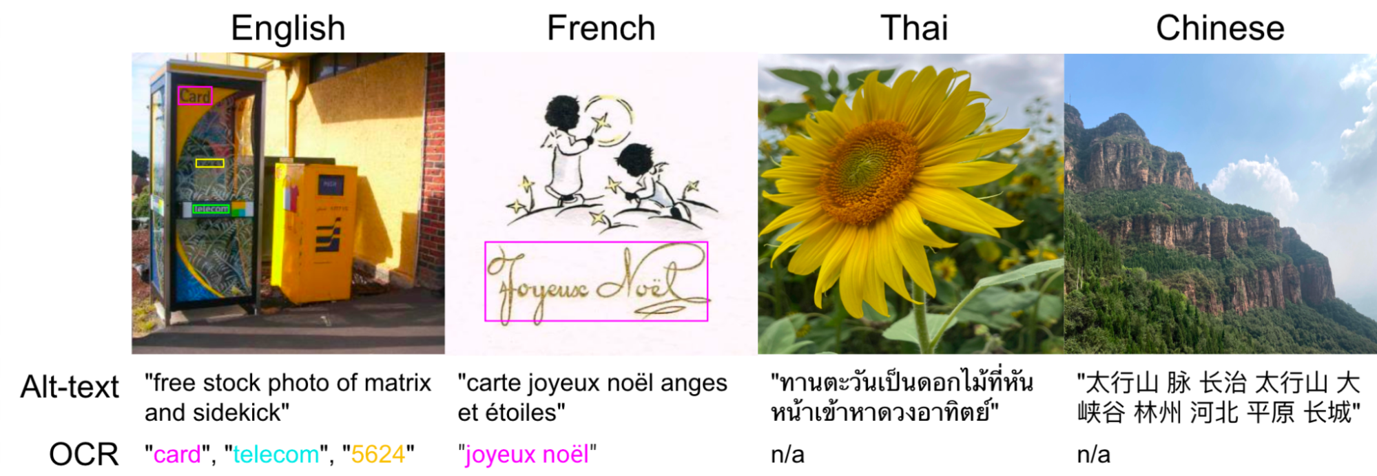
Sampled images from WebLI associated with multilingual alt-text and OCR. The second image is by jopradier (original), used under the CC BY-NC-SA 2.0 license. Remaining images are also used with permission.

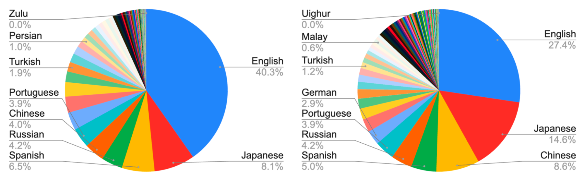
Statistics of recognized languages from alt-text and OCR in WebLI.

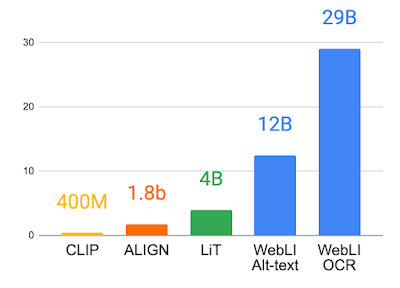
Image-text pair counts of WebLI and other large-scale vision-language datasets, CLIP, ALIGN and LiT.

Training Large Language-Image Models
Vision-language tasks require different capabilities and sometimes have diverging goals. Some tasks inherently require localization of objects to solve the task accurately, whereas some other tasks might need a more global view. Similarly, different tasks might require either long or compact answers. To address all of these objectives, we leverage the richness of the WebLI pre-training data and introduce a mixture of pre-training tasks, which prepare the model for a variety of downstream applications. To accomplish the goal of solving a wide variety of tasks, we enable knowledge-sharing between multiple image and language tasks by casting all tasks into a single generalized API (input: image + text; output: text), which is also shared with the pretraining setup. The objectives used for pre-training are cast into the same API as a weighted mixture aimed at both maintaining the ability of the reused model components and training the model to perform new tasks (e.g., split-captioning for image description, OCR prediction for scene-text comprehension, VQG and VQA prediction).

The model is trained in JAX with Flax using the open-sourced T5X and Flaxformer framework. For the visual component, we introduce and train a large ViT architecture, named ViT-e, with 4B parameters using the open-sourced BigVision framework. ViT-e follows the same recipe as the ViT-G architecture (which has 2B parameters). For the language component, we concatenate the dense token embeddings with the patch embeddings produced by the visual component, together as the input to the multimodal encoder-decoder, which is initialized from mT5-XXL. During the training of PaLI, the weights of this visual component are frozen, and only the weights of the multimodal encoder-decoder are updated.

Results
We compare PaLI on common vision-language benchmarks that are varied and challenging. The PaLI model achieves state-of-the-art results on these tasks, even outperforming very large models in the literature. For example, it outperforms the Flamingo model, which is several times larger (80B parameters), on several VQA and image-captioning tasks, and it also sustains performance on challenging language-only and vision-only tasks, which were not the main training objective.

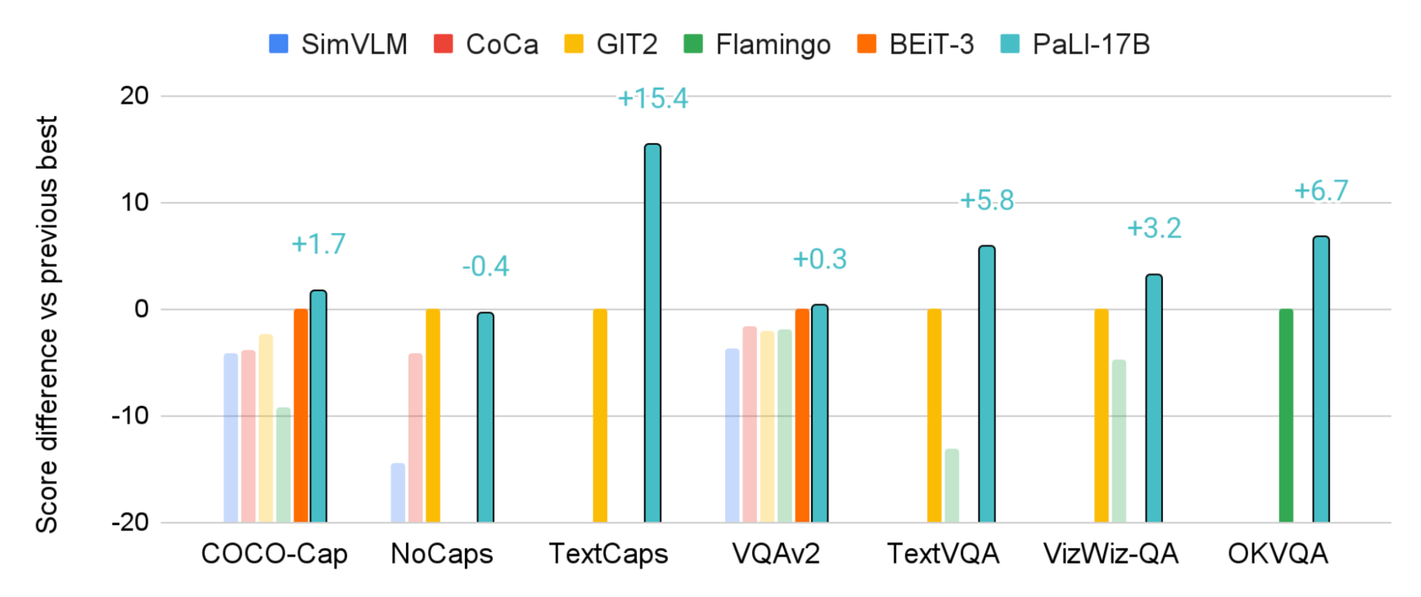
PaLI (17B parameters) outperforms the state-of-the-art approaches (including SimVLM, CoCa, GIT2, Flamingo, BEiT3) on multiple vision-and-language tasks. In this plot we show the absolute score differences compared with the previous best model to highlight the relative improvements of PaLI. Comparison is on the official test splits when available. CIDEr score is used for evaluation of the image captioning tasks, whereas VQA tasks are evaluated by VQA Accuracy.

Model Scaling Results
We examine how the image and language model components interact with each other with regards to model scaling and where the model yields the most gains. We conclude that scaling both components jointly results in the best performance, and specifically, scaling the visual component, which requires relatively few parameters, is most essential. Scaling is also critical for better performance across multilingual tasks.

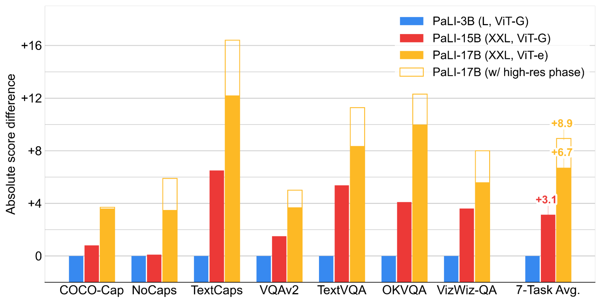
Scaling both the language and the visual components of the PaLI model contribute to improved performance. The plot shows the score differences compared to the PaLI-3B model: CIDEr score is used for evaluation of the image captioning tasks, whereas VQA tasks are evaluated by VQA Accuracy.

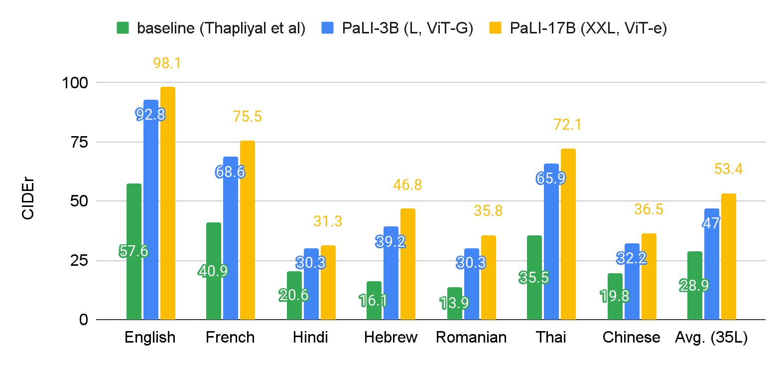
Multilingual captioning greatly benefits from scaling the PaLI models. We evaluate PaLI on a 35-language benchmark Crossmodal-3600. Here we present the average score over all 35 languages and the individual score for seven diverse languages.

Model Introspection: Model Fairness, Biases, and Other Potential Issues
To avoid creating or reinforcing unfair bias within large language and image models, important first steps are to (1) be transparent about the data that were used and how the model used those data, and (2) test for model fairness and conduct responsible data analyses. To address (1), our paper includes a data card and model card. To address (2), the paper includes results of demographic analyses of the dataset. We consider this a first step and know that it will be important to continue to measure and mitigate potential biases as we apply our model to new tasks, in alignment with our AI Principles.

Conclusion
We presented PaLI, a scalable multi-modal and multilingual model designed for solving a variety of vision-language tasks. We demonstrate improved performance across visual-, language- and vision-language tasks. Our work illustrates the importance of scale in both the visual and language parts of the model and the interplay between the two. We see that accomplishing vision and language tasks, especially in multiple languages, actually requires large scale models and data, and will potentially benefit from further scaling. We hope this work inspires further research in multi-modal and multilingual models.

Acknowledgements
We thank all the authors who conducted this research Soravit (Beer) Changpinyo, AJ Piergiovanni, Piotr Padlewski, Daniel Salz, Sebastian Goodman, Adam Grycner, Basil Mustafa, Lucas Beyer, Alexander Kolesnikov, Joan Puigcerver, Nan Ding, Keran Rong, Hassan Akbari,Gaurav Mishra, Linting Xue, Ashish Thapliyal, James Bradbury, Weicheng Kuo, Mojtaba Seyedhosseini, Chao Jia, Burcu Karagol Ayan, Carlos Riquelme, Andreas Steiner, Anelia Angelova, Xiaohua Zhai, Neil Houlsby, Radu Soricut. We also thank Claire Cui, Slav Petrov, Tania Bedrax-Weiss, Joelle Barral, Tom Duerig, Paul Natsev, Fernando Pereira, Jeff Dean, Jeremiah Harmsen, Zoubin Ghahramani, Erica Moreira, Victor Gomes, Sarah Laszlo, Kathy Meier-Hellstern, Susanna Ricco, Rich Lee, Austin Tarango, Emily Denton, Bo Pang, Wei Li, Jihyung Kil, Tomer Levinboim, Julien Amelot, Zhenhai Zhu, Xiangning Chen, Liang Chen, Filip Pavetic, Daniel Keysers, Matthias Minderer, Josip Djolonga, Ibrahim Alabdulmohsin, Mostafa Dehghani, Yi Tay, Elizabeth Adkison, James Cockerille, Eric Ni, Anna Davies, and Maysam Moussalem for their suggestions, improvements and support. We thank Tom Small for providing visualizations for the blogpost.

Source: Google AI Blog

LOLNeRF: Learn from One Look

Posted by Daniel Rebain, Student Researcher, and Mark Matthews, Senior Software Engineer, Google Research, Perception Team

An important aspect of human vision is our ability to comprehend 3D shape from the 2D images we observe. Achieving this kind of understanding with computer vision systems has been a fundamental challenge in the field. Many successful approaches rely on multi-view data, where two or more images of the same scene are available from different perspectives, which makes it much easier to infer the 3D shape of objects in the images.

There are, however, many situations where it would be useful to know 3D structure from a single image, but this problem is generally difficult or impossible to solve. For example, it isn’t necessarily possible to tell the difference between an image of an actual beach and an image of a flat poster of the same beach. However it is possible to estimate 3D structure based on what kind of 3D objects occur commonly and what similar structures look like from different perspectives.

In “LOLNeRF: Learn from One Look”, presented at CVPR 2022, we propose a framework that learns to model 3D structure and appearance from collections of single-view images. LOLNeRF learns the typical 3D structure of a class of objects, such as cars, human faces or cats, but only from single views of any one object, never the same object twice. We build our approach by combining Generative Latent Optimization (GLO) and neural radiance fields (NeRF) to achieve state-of-the-art results for novel view synthesis and competitive results for depth estimation.

We learn a 3D object model by reconstructing a large collection of single-view images using a neural network conditioned on latent vectors, z (left). This allows for a 3D model to be lifted from the image, and rendered from novel viewpoints. Holding the camera fixed, we can interpolate or sample novel identities (right).

Combining GLO and NeRF
GLO is a general method that learns to reconstruct a dataset (such as a set of 2D images) by co-learning a neural network (decoder) and table of codes (latents) that is also an input to the decoder. Each of these latent codes re-creates a single element (such as an image) from the dataset. Because the latent codes have fewer dimensions than the data elements themselves, the network is forced to generalize, learning common structure in the data (such as the general shape of dog snouts).

NeRF is a technique that is very good at reconstructing a static 3D object from 2D images. It represents an object with a neural network that outputs color and density for each point in 3D space. Color and density values are accumulated along rays, one ray for each pixel in a 2D image. These are then combined using standard computer graphics volume rendering to compute a final pixel color. Importantly, all these operations are differentiable, allowing for end-to-end supervision. By enforcing that each rendered pixel (of the 3D representation) matches the color of ground truth (2D) pixels, the neural network creates a 3D representation that can be rendered from any viewpoint.

We combine NeRF with GLO by assigning each object a latent code and concatenating it with standard NeRF inputs, giving it the ability to reconstruct multiple objects. Following GLO, we co-optimize these latent codes along with network weights during training to reconstruct the input images. Unlike standard NeRF, which requires multiple views of the same object, we supervise our method with only single views of any one object (but multiple examples of that type of object). Because NeRF is inherently 3D, we can then render the object from arbitrary viewpoints. Combining NeRF with GLO gives it the ability to learn common 3D structure across instances from only single views while still retaining the ability to recreate specific instances of the dataset.

Camera Estimation
In order for NeRF to work, it needs to know the exact camera location, relative to the object, for each image. Unless this was measured when the image was taken, it is generally unknown. Instead, we use the MediaPipe Face Mesh to extract five landmark locations from the images. Each of these 2D predictions correspond to a semantically consistent point on the object (e.g., the tip of the nose or corners of the eyes). We can then derive a set of canonical 3D locations for the semantic points, along with estimates of the camera poses for each image, such that the projection of the canonical points into the images is as consistent as possible with the 2D landmarks.

We train a per-image table of latent codes alongside a NeRF model. Output is subject to per-ray RGB, mask and hardness losses. Cameras are derived from a fit of predicted landmarks to canonical 3D keypoints.

Example MediaPipe landmarks and segmentation masks (images from CelebA).

Hard Surface and Mask Losses
Standard NeRF is effective for accurately reproducing the images, but in our single-view case, it tends to produce images that look blurry when viewed off-axis. To address this, we introduce a novel hard surface loss, which encourages the density to adopt sharp transitions from exterior to interior regions, reducing blurring. This essentially tells the network to create “solid” surfaces, and not semi-transparent ones like clouds.

We also obtained better results by splitting the network into separate foreground and background networks. We supervised this separation with a mask from the MediaPipe Selfie Segmenter and a loss to encourage network specialization. This allows the foreground network to specialize only on the object of interest, and not get “distracted” by the background, increasing its quality.

Results
We surprisingly found that fitting only five key points gave accurate enough camera estimates to train a model for cats, dogs, or human faces. This means that given only a single view of your beloved cats Schnitzel, Widget and friends, you can create a new image from any other angle.

Top: example cat images from AFHQ. Bottom: A synthesis of novel 3D views created by LOLNeRF.

Conclusion
We’ve developed a technique that is effective at discovering 3D structure from single 2D images. We see great potential in LOLNeRF for a variety of applications and are currently investigating potential use-cases.

Interpolation of feline identities from linear interpolation of learned latent codes for different examples in AFHQ.

Code Release
We acknowledge the potential for misuse and importance of acting responsibly. To that end, we will only release the code for reproducibility purposes, but will not release any trained generative models.

Acknowledgements
We would like to thank Andrea Tagliasacchi, Kwang Moo Yi, Viral Carpenter, David Fleet, Danica Matthews, Florian Schroff, Hartwig Adam and Dmitry Lagun for continuous help in building this technology.

Source: Google AI Blog

Accelerate your models to production with Google Cloud and PyTorch

We believe in the power of choice for Machine Learning development, and continue to invest resources to make it easy for ML practitioners to train, deploy, and orchestrate models from a single unified data and AI cloud platform. We’re excited to announce our role as a founding member of the newly formed PyTorch Foundation, which will better position Google Cloud to make meaningful contributions to the PyTorch community. As a member of the board, we will deepen our open source investment to deliver on the Foundation’s mission to drive adoption of AI tooling by building an ecosystem of open source projects with PyTorch. We strongly believe in choice and will continue to invest in frameworks such as JAX and Tensorflow and support integrations with other OSS Projects including Spark, Airflow, XGBoost, and others.

In this blog, we provide an overview of existing resources to help you get started with PyTorch on Google Cloud. We also talk about how ML practitioners can leverage our end-to-end ML platform to train, tune, and deploy PyTorch models.

PyTorch on Google Cloud

Open source in the cloud is important because it gives you flexibility and control over where you train and deploy your ML workloads. PyTorch is extensively used in the research space and in recent years it has gained immense traction in the industry due to its ease of use and deployment. In fact, according to a survey of Kaggle users, PyTorch is the fastest growing ML framework today.

ML practitioners using PyTorch tell us that it can be challenging to advance their ML project past experimentation. This is why Google Cloud has built integrations with PyTorch that make it easier to train, deploy, and orchestrate models in production. Some examples are:

PyTorch integrates directly with Vertex AI, a fully managed ML platform that provides the tools you need to take a model from PyTorch to production, like the Pytorch DL containers or the Vertex AI workbench PyTorch one-click JupyterLab environment.
PyTorch/XLA, an open source library, uses the XLA deep learning compiler to enable PyTorch to run on Cloud TPUs. Cloud TPUs are custom accelerators designed by Google, optimized for perf/TCO with large scale ML workload PyTorch/XLA also enables XLA driven optimizations on GPUs.
TorchX provides an adapter to run and orchestrate TorchX components as part of Kubeflow Pipelines that you can easily scale on Vertex AI Pipelines.
With our OSS contributions to Apache Beam, we have made PyTorch models easy to deploy in batch or stream, data processing pipelines. Running on Google Dataflow, these pipelines will scale to very large workloads in a fully managed and simple to maintain environment.

To learn more and start using PyTorch on Google Cloud, check out the resources below:

PyTorch on Vertex AI Resources

How To train and tune PyTorch models on Vertex AI: Learn how to use Vertex AI Training to build and train a sentiment text classification model using PyTorch and Vertex AI Hyperparameter Tuning to tune hyperparameters of PyTorch models.
How to deploy PyTorch models on Vertex AI: Walk through the deployment of a Pytorch model using TorchServe as a custom container, by deploying the model artifacts to a Vertex Prediction service.
Orchestrating PyTorch ML Workflows on Vertex AI Pipelines: See how to build and orchestrate ML pipelines for training and deploying PyTorch models on Google Cloud Vertex AI using Vertex AI Pipelines.
Scalable ML Workflows using PyTorch on Kubeflow Pipelines and Vertex Pipelines: Take a look at examples of PyTorch-based ML workflows on two pipelines frameworks: OSS Kubeflow Pipelines, part of the Kubeflow project, and Vertex AI Pipelines. We share new PyTorch built-in components added to the Kubeflow Pipelines.

PyTorch/XLA and Cloud TPU/GPU

Scaling deep learning workloads with PyTorch / XLA and Cloud TPU VM: Describes the challenges associated with scaling deep learning jobs to distributed training settings, using the Cloud TPU VM and shows how to stream training data from Google Cloud Storage (GCS) to PyTorch / XLA models running on Cloud TPU Pod slices.
PyTorch/XLA: Performance debugging on Cloud TPU VM: Part I: In the first part of the performance debugging series on Cloud TPU, we lay out the conceptual framework for PyTorch/XLA in the context of training performance. We introduced a case study to make sense of preliminary profiler logs and identify the corrective actions.
PyTorch/XLA: Performance debugging on Cloud TPU VM: Part II: In the second part, we deep dive into further analysis of the performance debugging to discover more performance improvement opportunities.
PyTorch/XLA: Performance debugging on Cloud TPU VM: Part III: In the final part of the performance debugging series, we introduce user defined code annotation and visualize these annotations in the form of a trace.
Train ML models with Pytorch Lightning on TPUs: Learn how easy it is to start training models with PyTorch Lightning on TPUs with its built-in TPU support.

Other resources

Increase your productivity using PyTorch Lightning: Learn how to use PyTorch Lightning on Vertex AI Workbench (was previously Notebooks).

By Erwin Huizing and Grace Reed – Cloud AI and ML

Source: Google Open Source Blog

A Multi-Axis Approach for Vision Transformer and MLP Models

Posted by Zhengzhong Tu and Yinxiao Li, Software Engineers, Google Research

Convolutional neural networks have been the dominant machine learning architecture for computer vision since the introduction of AlexNet in 2012. Recently, inspired by the evolution of Transformers in natural language processing, attention mechanisms have been prominently incorporated into vision models. These attention methods boost some parts of the input data while minimizing other parts so that the network can focus on small but important parts of the data. The Vision Transformer (ViT) has created a new landscape of model designs for computer vision that is completely free of convolution. ViT regards image patches as a sequence of words, and applies a Transformer encoder on top. When trained on sufficiently large datasets, ViT demonstrates compelling performance on image recognition.

While convolutions and attention are both sufficient for good performance, neither of them are necessary. For example, MLP-Mixer adopts a simple multi-layer perceptron (MLP) to mix image patches across all the spatial locations, resulting in an all-MLP architecture. It is a competitive alternative to existing state-of-the-art vision models in terms of the trade-off between accuracy and computation required for training and inference. However, both ViT and the MLP models struggle to scale to higher input resolution because the computational complexity increases quadratically with respect to the image size.

Today we present a new multi-axis approach that is simple and effective, improves on the original ViT and MLP models, can better adapt to high-resolution, dense prediction tasks, and can naturally adapt to different input sizes with high flexibility and low complexity. Based on this approach, we have built two backbone models for high-level and low-level vision tasks. We describe the first in “MaxViT: Multi-Axis Vision Transformer”, to be presented in ECCV 2022, and show it significantly improves the state of the art for high-level tasks, such as image classification, object detection, segmentation, quality assessment, and generation. The second, presented in “MAXIM: Multi-Axis MLP for Image Processing” at CVPR 2022, is based on a UNet-like architecture and achieves competitive performance on low-level imaging tasks including denoising, deblurring, dehazing, deraining, and low-light enhancement. To facilitate further research on efficient Transformer and MLP models, we have open-sourced the code and models for both MaxViT and MAXIM.

A demo of image deblurring using MAXIM frame by frame.

Overview
Our new approach is based on multi-axis attention, which decomposes the full-size attention (each pixel attends to all the pixels) used in ViT into two sparse forms — local and (sparse) global. As shown in the figure below, the multi-axis attention contains a sequential stack of block attention and grid attention. The block attention works within non-overlapping windows (small patches in intermediate feature maps) to capture local patterns, while the grid attention works on a sparsely sampled uniform grid for long-range (global) interactions. The window sizes of grid and block attentions can be fully controlled as hyperparameters to ensure a linear computational complexity to the input size.

The proposed multi-axis attention conducts blocked local and dilated global attention sequentially followed by a FFN, with only a linear complexity. The pixels in the same colors are attended together.

Such low-complexity attention can significantly improve its wide applicability to many vision tasks, especially for high-resolution visual predictions, demonstrating greater generality than the original attention used in ViT. We build two backbone instantiations out of this multi-axis attention approach – MaxViT and MAXIM, for high-level and low-level tasks, respectively.

MaxViT
In MaxViT, we first build a single MaxViT block (shown below) by concatenating MBConv (proposed by EfficientNet, V2) with the multi-axis attention. This single block can encode local and global visual information regardless of input resolution. We then simply stack repeated blocks composed of attention and convolutions in a hierarchical architecture (similar to ResNet, CoAtNet), yielding our homogenous MaxViT architecture. Notably, MaxViT is distinguished from previous hierarchical approaches as it can “see” globally throughout the entire network, even in earlier, high-resolution stages, demonstrating stronger model capacity on various tasks.

The meta-architecture of MaxViT.

MAXIM
Our second backbone, MAXIM, is a generic UNet-like architecture tailored for low-level image-to-image prediction tasks. MAXIM explores parallel designs of the local and global approaches using the gated multi-layer perceptron (gMLP) network (patching-mixing MLP with a gating mechanism). Another contribution of MAXIM is the cross-gating block that can be used to apply interactions between two different input signals. This block can serve as an efficient alternative to the cross-attention module as it only employs the cheap gated MLP operators to interact with various inputs without relying on the computationally heavy cross-attention. Moreover, all the proposed components including the gated MLP and cross-gating blocks in MAXIM enjoy linear complexity to image size, making it even more efficient when processing high-resolution pictures.

Results
We demonstrate the effectiveness of MaxViT on a broad range of vision tasks. On image classification, MaxViT achieves state-of-the-art results under various settings: with only ImageNet-1K training, MaxViT attains 86.5% top-1 accuracy; with ImageNet-21K (14M images, 21k classes) pre-training, MaxViT achieves 88.7% top-1 accuracy; and with JFT (300M images, 18k classes) pre-training, our largest model MaxViT-XL achieves a high accuracy of 89.5% with 475M parameters.

Performance comparison of MaxViT with state-of-the-art models on ImageNet-1K. Top: Accuracy vs. FLOPs performance scaling with 224x224 image resolution. Bottom: Accuracy vs. parameters scaling curve under ImageNet-1K fine-tuning setting.

For downstream tasks, MaxViT as a backbone delivers favorable performance on a broad spectrum of tasks. For object detection and segmentation on the COCO dataset, the MaxViT backbone achieves 53.4 AP, outperforming other base-level models while requiring only about 60% the computational cost. For image aesthetics assessment, the MaxViT model advances the state-of-the-art MUSIQ model by 3.5% in terms of linear correlation with human opinion scores. The standalone MaxViT building block also demonstrates effective performance on image generation, achieving better FID and IS scores on the ImageNet-1K unconditional generation task with a significantly lower number of parameters than the state-of-the-art model, HiT.

The UNet-like MAXIM backbone, customized for image processing tasks, has also demonstrated state-of-the-art results on 15 out of 20 tested datasets, including denoising, deblurring, deraining, dehazing, and low-light enhancement, while requiring fewer or comparable number of parameters and FLOPs than competitive models. Images restored by MAXIM show more recovered details with less visual artifacts.

Visual results of MAXIM for image deblurring, deraining, and low-light enhancement.

Summary
Recent works in the last two or so years have shown that ConvNets and Vision Transformers can achieve similar performance. Our work presents a unified design that takes advantage of the best of both worlds — efficient convolution and sparse attention — and demonstrates that a model built on top, namely MaxViT, can achieve state-of-the-art performance on a variety of vision tasks. More importantly, MaxViT scales well to very large data sizes. We also show that an alternative multi-axis design using MLP operators, MAXIM, achieves state-of-the-art performance on a broad range of low-level vision tasks.

Even though we present our models in the context of vision tasks, the proposed multi-axis approach can easily extend to language modeling to capture both local and global dependencies in linear time. Motivated by the work here, we expect that it is worthwhile to study other forms of sparse attention in higher-dimensional or multimodal signals such as videos, point clouds, and vision-language models.

We have open-sourced the code and models of MAXIM and MaxViT to facilitate future research on efficient attention and MLP models.

Acknowledgments
We would like to thank our co-authors: Hossein Talebi, Han Zhang, Feng Yang, Peyman Milanfar, and Alan Bovik. We would also like to acknowledge the valuable discussion and support from Xianzhi Du, Long Zhao, Wuyang Chen, Hanxiao Liu, Zihang Dai, Anurag Arnab, Sungjoon Choi, Junjie Ke, Mauricio Delbracio, Irene Zhu, Innfarn Yoo, Huiwen Chang, and Ce Liu.