Tag Archives: Google Maps
Introducing Google Maps Platform
Posted by Google Maps Platform Team
It's been thirteen years since we opened up Google Maps to your creativity and passion. Since then, it's been exciting to see how you've transformed your industries and improved people's lives. You've changed the way we ride to work, discover the best schools for our children, and search for a new place to live. We can't wait to see what you do next. That's why today we're introducing a series of updates designed to make it easier for you to start taking advantage of new location-based features and products.
We're excited to announce Google Maps Platform—the next generation of our Google Maps business—encompassing streamlined API products and new industry solutions to help drive innovation.
In March, we announced our first industry solution for game studios to create real-world games using Google Maps data. Today, we also offer solutions tailored for ridesharing and asset tracking companies. Ridesharing companies can embed the Google Maps navigation experience directly into their apps to optimize the driver and customer experience. Our asset tracking offering helps businesses improve efficiencies by locating vehicles and assets in real-time, visualizing where assets have traveled, and routing vehicles with complex trips. We expect to bring new solutions to market in the future, in areas where we're positioned to offer insights and expertise.
Our core APIs work together to provide the building blocks you need to create location-based apps and experiences. One of our goals is to evolve our core APIs to make them simpler, easier to use and scalable as you grow. That's why we've introduced a number of updates to help you do so.
Streamlined products to create new location-based experiences
We're simplifying our 18 individual APIs into three core products—Maps, Routes and Places, to make it easier for you to find, explore and add new features to your apps and sites. And, these new updates will work with your existing code—no changes required.
One pricing plan, free support, and a single console
We've heard that you want simple, easy to understand pricing that gives you access to all our core APIs. That's one of the reasons we merged our Standard and Premium plans to form one pay-as-you go pricing plan for our core products. With this new plan, developers will receive the first $200 of monthly usage for free. We estimate that most of you will have monthly usage that will keep you within this free tier. With this new pricing plan you'll pay only for the services you use each month with no annual, up-front commitments, termination fees or usage limits. And we're rolling out free customer support for all. In addition, our products are now integrated with Google Cloud Platform Console to make it easier for you to track your usage, manage your projects, and discover new innovative Cloud products.
Scale easily as you grow
Beginning June 11, you'll need a valid API key and a Google Cloud Platform billing account to access our core products. Once you enable billing, you will gain access to your $200 of free monthly usage to use for our Maps, Routes, and Places products. As your business grows or usage spikes, our plan will scale with you. And, with Google Maps' global infrastructure, you can scale without thinking about capacity, reliability, or performance. We'll continue to partner with Google programs that bring our products to nonprofits, startups, crisis response, and news media organizations. We've put new processes in place to help us scale these programs to hundreds of thousands of organizations and more countries around the world.
We're excited about all the new location-based experiences you'll build, and we want to be there to support you along the way. If you're currently using our core APIs, please take a look at our Guide for Existing Users to further understand these changes and help you easily transition to the new plan. And if you're just getting started, you can start your first project here. We're here to help.
Source: Google Developers Blog
Balanced Partitioning and Hierarchical Clustering at Scale
Solving large-scale optimization problems often starts with graph partitioning, which means partitioning the vertices of the graph into clusters to be processed on different machines. The need to make sure that clusters are of near equal size gives rise to the balanced graph partitioning problem. In simple terms, we need to partition the vertices of a given graph into k almost equal clusters, while we minimize the number of edges that are cut by the partition. This NP-hard problem is notoriously difficult in practice because the best approximation algorithms for small instances rely on semidefinite programming which is impractical for larger instances.
This post presents the distributed algorithm we developed which is more applicable to large instances. We introduced this balanced graph-partitioning algorithm in our WSDM 2016 paper, and have applied this approach to several applications within Google. Our more recent NIPS 2017 paper provides more details of the algorithm via a theoretical and empirical study.
Balanced Partitioning via Linear Embedding
Our algorithm first embeds vertices of the graph onto a line, and then processes vertices in a distributed manner guided by the linear embedding order. We examine various ways to find the initial embedding, and apply four different techniques (such as local swaps and dynamic programming) to obtain the final partition. The best initial embedding is based on “affinity clustering”.
Affinity Hierarchical Clustering
Affinity clustering is an agglomerative hierarchical graph clustering based on Borůvka’s classic Maximum-cost Spanning Tree algorithm. As discussed above, this algorithm is a critical part of our balanced partitioning tool. The algorithm starts by placing each vertex in a cluster of its own: v0, v1, and so on. Then, in each iteration, the highest-cost edge out of each cluster is selected in order to induce larger merged clusters: A0, A1, A2, etc. in the first round and B0, B1, etc. in the second round and so on. The set of merges naturally produces a hierarchical clustering, and gives rise to a linear ordering of the leaf vertices (vertices with degree one). The image below demonstrates this, with the numbers at the bottom corresponding to the ordering of the vertices.
Our NIPS’17 paper explains how we run affinity clustering efficiently in the massively parallel computation (MPC) model, in particular using distributed hash tables (DHTs) to significantly reduce running time. This paper also presents a theoretical study of the algorithm. We report clustering results for graphs with tens of trillions of edges, and also observe that affinity clustering empirically beats other clustering algorithms such as k-means in terms of “quality of the clusters”. This video contains a summary of the result and explains how this parallel algorithm may produce higher-quality clusters even compared to a sequential single-linkage agglomerative algorithm.
Comparison to Previous Work
In comparing our algorithm to previous work in (distributed) balanced graph partitioning, we focus on FENNEL, Spinner, METIS, and a recent label propagation-based algorithm. We report results on several public social networks as well as a large private map graph. For a Twitter followership graph, we see a consistent improvement of 15–25% over previous results (Ugander and Backstrom, 2013), and for LiveJournal graph, our algorithm outperforms all the others for all cases except k = 2, where ours is slightly worse than FENNEL's.
The following table presents the fraction of cut edges in the Twitter graph obtained via different algorithms for various values of k, the number of clusters. The numbers given in parentheses denote the size imbalance factor: i.e., the relative difference of the sizes of largest and smallest clusters. Here “Vanilla Affinity Clustering” denotes the first stage of our algorithm where only the hierarchical clustering is built and no further processing is performed on the cuts. Notice that this is already as good as the best previous work (shown in the first two columns below), cutting a smaller fraction of edges while achieving a perfect (and thus better) balance (i.e., 0% imbalance). The last column in the table includes the final result of our algorithm with the post-processing.
k | UB13 (5%) | Spinner (5%) | Vanilla Affinity Clustering (0%) | Final Algorithm (0%) |
20 | 37.0% | 38.0% | 35.71% | 27.50% |
40 | 43.0% | 40.0% | 40.83% | 33.71% |
60 | 46.0% | 43.0% | 43.03% | 36.65% |
80 | 47.5% | 44.0% | 43.27% | 38.65% |
100 | 49.0% | 46.0% | 45.05% | 41.53% |
Applications
We apply balanced graph partitioning to multiple applications including Google Maps driving directions, the serving backend for web search, and finding treatment groups for experimental design. For example, in Google Maps the World map graph is stored in several shards. The navigational queries spanning multiple shards are substantially more expensive than those handled within a shard. Using the methods described in our paper, we can reduce 21% of cross-shard queries by increasing the shard imbalance factor from 0% to 10%. As discussed in our paper, live experiments on real traffic show that the number of multi-shard queries from our cut-optimization techniques is 40% less compared to a baseline Hilbert embedding technique. This, in turn, results in less CPU usage in response to queries. In a future blog post, we will talk about application of this work in the web search serving backend, where balanced partitioning helped us design a cache-aware load balancing system that dramatically reduced our cache miss rate.
Acknowledgements
We especially thank Vahab Mirrokni whose guidance and technical contribution were instrumental in developing these algorithms and writing this post. We also thank our other co-authors and colleagues for their contributions: Raimondas Kiveris, Soheil Behnezhad, Mahsa Derakhshan, MohammadTaghi Hajiaghayi, Silvio Lattanzi, Aaron Archer and other members of NYC Algorithms and Optimization research team.
Source: Google Research Blog
Balanced Partitioning and Hierarchical Clustering at Scale
Solving large-scale optimization problems often starts with graph partitioning, which means partitioning the vertices of the graph into clusters to be processed on different machines. The need to make sure that clusters are of near equal size gives rise to the balanced graph partitioning problem. In simple terms, we need to partition the vertices of a given graph into k almost equal clusters, while we minimize the number of edges that are cut by the partition. This NP-hard problem is notoriously difficult in practice because the best approximation algorithms for small instances rely on semidefinite programming which is impractical for larger instances.
This post presents the distributed algorithm we developed which is more applicable to large instances. We introduced this balanced graph-partitioning algorithm in our WSDM 2016 paper, and have applied this approach to several applications within Google. Our more recent NIPS 2017 paper provides more details of the algorithm via a theoretical and empirical study.
Balanced Partitioning via Linear Embedding
Our algorithm first embeds vertices of the graph onto a line, and then processes vertices in a distributed manner guided by the linear embedding order. We examine various ways to find the initial embedding, and apply four different techniques (such as local swaps and dynamic programming) to obtain the final partition. The best initial embedding is based on “affinity clustering”.
Affinity Hierarchical Clustering
Affinity clustering is an agglomerative hierarchical graph clustering based on Borůvka’s classic Maximum-cost Spanning Tree algorithm. As discussed above, this algorithm is a critical part of our balanced partitioning tool. The algorithm starts by placing each vertex in a cluster of its own: v0, v1, and so on. Then, in each iteration, the highest-cost edge out of each cluster is selected in order to induce larger merged clusters: A0, A1, A2, etc. in the first round and B0, B1, etc. in the second round and so on. The set of merges naturally produces a hierarchical clustering, and gives rise to a linear ordering of the leaf vertices (vertices with degree one). The image below demonstrates this, with the numbers at the bottom corresponding to the ordering of the vertices.
Our NIPS’17 paper explains how we run affinity clustering efficiently in the massively parallel computation (MPC) model, in particular using distributed hash tables (DHTs) to significantly reduce running time. This paper also presents a theoretical study of the algorithm. We report clustering results for graphs with tens of trillions of edges, and also observe that affinity clustering empirically beats other clustering algorithms such as k-means in terms of “quality of the clusters”. This video contains a summary of the result and explains how this parallel algorithm may produce higher-quality clusters even compared to a sequential single-linkage agglomerative algorithm.
Comparison to Previous Work
In comparing our algorithm to previous work in (distributed) balanced graph partitioning, we focus on FENNEL, Spinner, METIS, and a recent label propagation-based algorithm. We report results on several public social networks as well as a large private map graph. For a Twitter followership graph, we see a consistent improvement of 15–25% over previous results (Ugander and Backstrom, 2013), and for LiveJournal graph, our algorithm outperforms all the others for all cases except k = 2, where ours is slightly worse than FENNEL's.
The following table presents the fraction of cut edges in the Twitter graph obtained via different algorithms for various values of k, the number of clusters. The numbers given in parentheses denote the size imbalance factor: i.e., the relative difference of the sizes of largest and smallest clusters. Here “Vanilla Affinity Clustering” denotes the first stage of our algorithm where only the hierarchical clustering is built and no further processing is performed on the cuts. Notice that this is already as good as the best previous work (shown in the first two columns below), cutting a smaller fraction of edges while achieving a perfect (and thus better) balance (i.e., 0% imbalance). The last column in the table includes the final result of our algorithm with the post-processing.
k | UB13 (5%) | Spinner (5%) | Vanilla Affinity Clustering (0%) | Final Algorithm (0%) |
20 | 37.0% | 38.0% | 35.71% | 27.50% |
40 | 43.0% | 40.0% | 40.83% | 33.71% |
60 | 46.0% | 43.0% | 43.03% | 36.65% |
80 | 47.5% | 44.0% | 43.27% | 38.65% |
100 | 49.0% | 46.0% | 45.05% | 41.53% |
Applications
We apply balanced graph partitioning to multiple applications including Google Maps driving directions, the serving backend for web search, and finding treatment groups for experimental design. For example, in Google Maps the World map graph is stored in several shards. The navigational queries spanning multiple shards are substantially more expensive than those handled within a shard. Using the methods described in our paper, we can reduce 21% of cross-shard queries by increasing the shard imbalance factor from 0% to 10%. As discussed in our paper, live experiments on real traffic show that the number of multi-shard queries from our cut-optimization techniques is 40% less compared to a baseline Hilbert embedding technique. This, in turn, results in less CPU usage in response to queries. In a future blog post, we will talk about application of this work in the web search serving backend, where balanced partitioning helped us design a cache-aware load balancing system that dramatically reduced our cache miss rate.
Acknowledgements
We especially thank Vahab Mirrokni whose guidance and technical contribution were instrumental in developing these algorithms and writing this post. We also thank our other co-authors and colleagues for their contributions: Raimondas Kiveris, Soheil Behnezhad, Mahsa Derakhshan, MohammadTaghi Hajiaghayi, Silvio Lattanzi, Aaron Archer and other members of NYC Algorithms and Optimization research team.
Source: Google AI Blog
Seamless Google Street View Panoramas
In 2007, we introduced Google Street View, enabling you to explore the world through panoramas of neighborhoods, landmarks, museums and more, right from your browser or mobile device. The creation of these panoramas is a complicated process, involving capturing images from a multi-camera rig called a rosette, and then using image blending techniques to carefully stitch them all together. However, many things can thwart the creation of a "successful" panorama, such as mis-calibration of the rosette camera geometry, timing differences between adjacent cameras, and parallax. And while we attempt to address these issues by using approximate scene geometry to account for parallax and frequent camera re-calibration, visible seams in image overlap regions can still occur.
 |
| Left: The Sydney Opera House with stitching seams along its iconic shells. Right: The same Street View panorama after optical flow seam repair. |
Optical Flow
The first step is to find corresponding pixel locations for each pair of images that overlap. Using techniques described in our PhotoScan blog post, we compute optical flow from one image to the other. This provides a smooth and dense correspondence field. We then downsample the correspondences for computational efficiency. We also discard correspondences where there isn’t enough visual structure to be confident in the results of optical flow.
 |
The boundaries of a pair of constituent images from the rosette camera rig that need to be stitched together. |
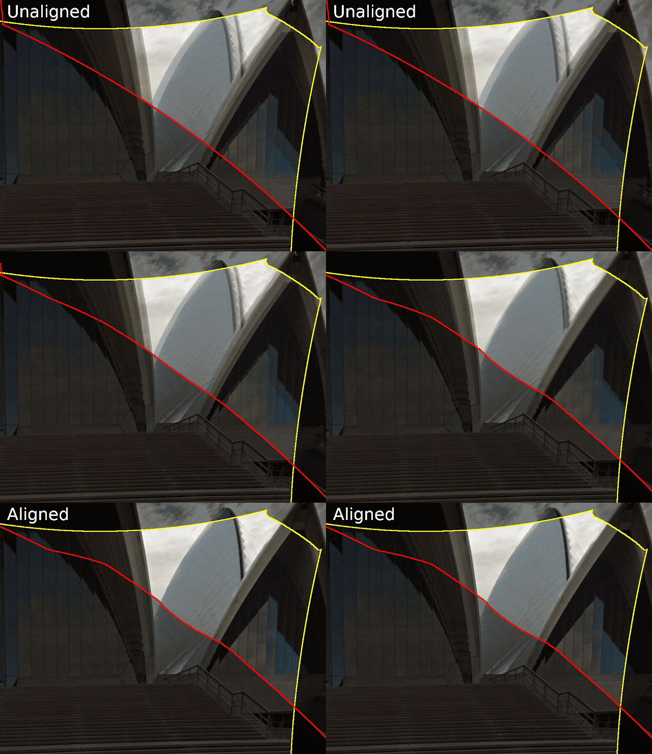 |
| An illustration of optical flow within the pair’s overlap region. |
The second step is to warp the rosette’s images to simultaneously align all of the corresponding points from overlap regions (as seen in the figure above). When stitched into a panorama, the set of warped images will then properly align. This is challenging because the overlap regions cover only a small fraction of each image, resulting in an under-constrained problem. To generate visually pleasing results across the whole image, we formulate the warping as a spline-based flow field with spatial regularization. The spline parameters are solved for in a non-linear optimization using Google’s open source Ceres Solver.
previously published work by Shum & Szeliski on “deghosting” panoramas. Key differences include that our approach estimates dense, smooth correspondences (rather than patch-wise, independent correspondences), and we solve a nonlinear optimization for the final warping. The result is a more well-behaved warping that is less likely to introduce new visual artifacts than the kernel-based approach.
 |
| Tower Bridge, London |
 |
| Christ the Redeemer, Rio de Janeiro |
 |
| An SUV on the streets of Seattle |
Acknowledgements
Special thanks to Bryan Klingner for helping to integrate this feature with the Street View infrastructure.
Source: Google Research Blog
Answer customer questions on Google
- Add frequently asked questions to your listing so that mobile users who find your business on Google Search and Google Maps can easily get the answers to your customers’ most common questions.
- Answer questions from potential customers on Google Search and Google Maps on your mobile phone. If you have Google Maps on Android, we‘ll also send you a push notification when a new question has been asked about your business so you can post an answer instantly.
- Highlight top responses. Beyond FAQs and your own responses, customers are also able to answer each other’s questions. You can highlight the most helpful answers from your customer community by using the thumb to bump them up to the top of the list.
Source: Google Small Business
Using Deep Learning to Create Professional-Level Photographs
Machine learning (ML) excels in many areas with well defined goals. Tasks where there exists a right or wrong answer help with the training process and allow the algorithm to achieve its desired goal, whether it be correctly identifying objects in images or providing a suitable translation from one language to another. However, there are areas where objective evaluations are not available. For example, whether a photograph is beautiful is measured by its aesthetic value, which is a highly subjective concept.
 |
| A professional(?) photograph of Jasper National Park, Canada. |
Training the Model
While aesthetics can be modelled using datasets like AVA, using it naively to enhance photos may miss some aspect in aesthetics, such as making a photo over-saturated. Using supervised learning to learn multiple aspects in aesthetics properly, however, may require a labelled dataset that is intractable to collect.
Our approach relies only on a collection of professional quality photos, without before/after image pairs, or any additional labels. It breaks down aesthetics into multiple aspects automatically, each of which is learned individually with negative examples generated by a coupled image operation. By keeping these image operations semi-”orthogonal”, we can enhance a photo on its composition, saturation/HDR level and dramatic lighting with fast and separable optimizations:
 |
| A panorama (a) is cropped into (b), with saturation and HDR strength enhanced in (c), and with dramatic mask applied in (d). Each step is guided by one learned aspect of aesthetics. |
Results
Some creations of our system from Google Street View are shown below. As you can see, the application of the trained aesthetic filters creates some dramatic results (including the image we started this post with!):
 |
| Jasper National Park, Canada. |
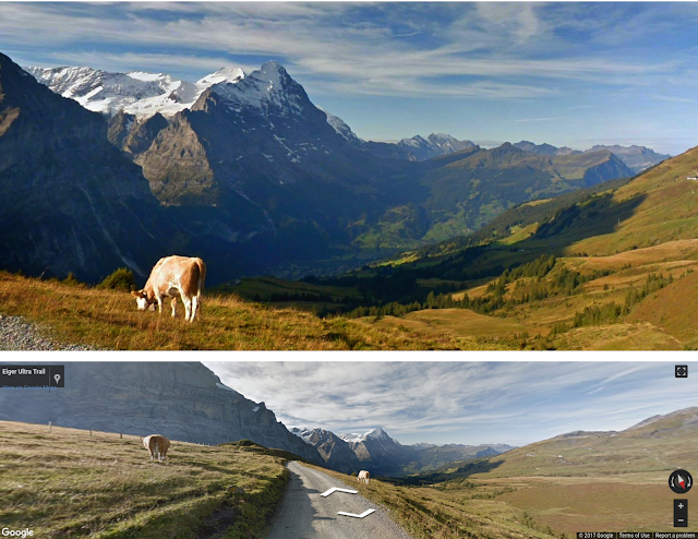 |
| Interlaken, Switzerland. |
 |
| Park Parco delle Orobie Bergamasche, Italy. |
 |
| Jasper National Park, Canada. |
To judge how successful our algorithm was, we designed a “Turing-test”-like experiment: we mix our creations with other photos at different quality, and show them to several professional photographers. They were instructed to assign a quality score for each of them, with meaning defined as following:
- 1: Point-and-shoot without consideration for composition, lighting etc.
- 2: Good photos from general population without a background in photography. Nothing artistic stands out.
- 3: Semi-pro. Great photos showing clear artistic aspects. The photographer is on the right track of becoming a professional.
- 4: Pro.
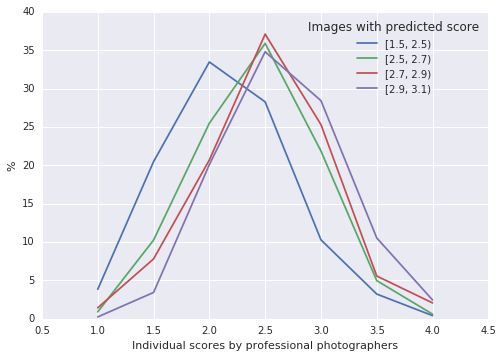 |
| Scores received from professional photographers for photos with different predicted scores. |
The Street View panoramas served as a testing bed for our project. Someday this technique might even help you to take better photos in the real world. We compiled a showcase of photos created to our satisfaction. If you see a photo you like, you can click on it to bring out a nearby Street View panorama. Would you make the same decision if you were there holding the camera at that moment?
Acknowledgements
This work was done by Hui Fang and Meng Zhang from Machine Perception at Google Research. We would like to thank Vahid Kazemi for his earlier work in predicting AVA scores using Inception network, and Sagarika Chalasani, Nick Beato, Bryan Klingner and Rupert Breheny for their help in processing Google Street View panoramas. We would like to thank Peyman Milanfar, Tomas Izo, Christian Szegedy, Jon Barron and Sergey Ioffe for their helpful reviews and comments. Huge thanks to our anonymous professional photographers!
Source: Google Research Blog
Make your business stand out on Google with Posts
Posts appear on your Google business listing. Customers can tap to read the full post, and they can also share your post with their friends directly from Google. | |
Posting on Google gives you new ways to engage with your customers:
- Share daily specials or current promotions that encourage new and existing customers to take advantage of your offers.
- Promote events and tell customers about upcoming happenings at your location.
- Showcase your top products and highlight new arrivals.
- Choose one of the available options to connect with your customers directly from your Google listing: give them a one-click path to make a reservation, sign up for a newsletter, learn more about latest offers, or even buy a specific product from your website.
Seventy percent of people look at multiple businesses before making a final choice.2 With Posts, you can share timely, relevant updates right on Google Search and Maps to help your business stand out to potential customers. And by including custom calls-to-action directly on your business listing, you can choose how to connect with your customers.
“Posts definitely helped our business because a lot of people look us up through Google. When they do, they want to see the vibe of the place. Being able to post directly to Google allows them to see the reviews and get a feel for the shop all in one spot.” - Cut & Grind, London, UK | “As a small business, we don’t have a ton of resources. We post with the intention of engaging new and existing customers, informing them of new therapists and services we offer as we expand our business. The posts help us stand out in a unique way and allow us to differentiate ourselves from our competition.” - Just Mind, Austin, TX | “Posts are worth my time because with limited effort you can get something fresh that is reaching people's eyes. 1,100 people saw my last post. Getting information out to the customers is big for this kind of business, letting them know we have bikes or different sporting goods they may not be aware of.”- Play It Again Sports, Saint Paul, MN |
If you’re not yet using Google My Business, sign up and get started today managing your business listing on Google. Once you’ve verified your business, you’ll be ready to start posting. To learn more, visit the Google My Business Help Center.


