Tag Archives: Google Brain

Eager Execution: An imperative, define-by-run interface to TensorFlow


Today, we introduce eager execution for TensorFlow. Eager execution is an imperative, define-by-run interface where operations are executed immediately as they are called from Python. This makes it easier to get started with TensorFlow, and can make research and development more intuitive.

The benefits of eager execution include:
  • Fast debugging with immediate run-time errors and integration with Python tools
  • Support for dynamic models using easy-to-use Python control flow
  • Strong support for custom and higher-order gradients
  • Almost all of the available TensorFlow operations
Eager execution is available now as an experimental feature, so we're looking for feedback from the community to guide our direction.

To understand this all better, let's look at some code. This gets pretty technical; familiarity with TensorFlow will help.

Using Eager Execution

When you enable eager execution, operations execute immediately and return their values to Python without requiring a Session.run(). For example, to multiply two matrices together, we write this:
import tensorflow as tf
import tensorflow.contrib.eager as tfe

tfe.enable_eager_execution()

x = [[2.]]
m = tf.matmul(x, x)
It’s straightforward to inspect intermediate results with print or the Python debugger.
print(m)
# The 1x1 matrix [[4.]]
Dynamic models can be built with Python flow control. Here's an example of the Collatz conjecture using TensorFlow’s arithmetic operations:
a = tf.constant(12)
counter = 0
while not tf.equal(a, 1):
if tf.equal(a % 2, 0):
a = a / 2
else:
a = 3 * a + 1
print(a)
Here, the use of the tf.constant(12) Tensor object will promote all math operations to tensor operations, and as such all return values with be tensors.

Gradients

Most TensorFlow users are interested in automatic differentiation. Because different operations can occur during each call, we record all forward operations to a tape, which is then played backwards when computing gradients. After we've computed the gradients, we discard the tape.

If you’re familiar with the autograd package, the API is very similar. For example:
def square(x):
return tf.multiply(x, x)

grad = tfe.gradients_function(square)

print(square(3.)) # [9.]
print(grad(3.)) # [6.]
The gradients_function call takes a Python function square() as an argument and returns a Python callable that computes the partial derivatives of square() with respect to its inputs. So, to get the derivative of square() at 3.0, invoke grad(3.0), which is 6.

The same gradients_function call can be used to get the second derivative of square:
gradgrad = tfe.gradients_function(lambda x: grad(x)[0])

print(gradgrad(3.)) # [2.]
As we noted, control flow can cause different operations to run, such as in this example.
def abs(x):
return x if x > 0. else -x

grad = tfe.gradients_function(abs)

print(grad(2.0)) # [1.]
print(grad(-2.0)) # [-1.]

Custom Gradients

Users may want to define custom gradients for an operation, or for a function. This may be useful for multiple reasons, including providing a more efficient or more numerically stable gradient for a sequence of operations.

Here is an example that illustrates the use of custom gradients. Let's start by looking at the function log(1 + ex), which commonly occurs in the computation of cross entropy and log likelihoods.
def log1pexp(x):
return tf.log(1 + tf.exp(x))
grad_log1pexp = tfe.gradients_function(log1pexp)

# The gradient computation works fine at x = 0.
print(grad_log1pexp(0.))
# [0.5]
# However it returns a `nan` at x = 100 due to numerical instability.
print(grad_log1pexp(100.))
# [nan]
We can use a custom gradient for the above function that analytically simplifies the gradient expression. Notice how the gradient function implementation below reuses an expression (tf.exp(x)) that was computed during the forward pass, making the gradient computation more efficient by avoiding redundant computation.
@tfe.custom_gradient
def log1pexp(x):
e = tf.exp(x)
def grad(dy):
return dy * (1 - 1 / (1 + e))
return tf.log(1 + e), grad
grad_log1pexp = tfe.gradients_function(log1pexp)

# Gradient at x = 0 works as before.
print(grad_log1pexp(0.))
# [0.5]
# And now gradient computation at x=100 works as well.
print(grad_log1pexp(100.))
# [1.0]

Building models

Models can be organized in classes. Here's a model class that creates a (simple) two layer network that can classify the standard MNIST handwritten digits.
class MNISTModel(tfe.Network):
def __init__(self):
super(MNISTModel, self).__init__()
self.layer1 = self.track_layer(tf.layers.Dense(units=10))
self.layer2 = self.track_layer(tf.layers.Dense(units=10))
def call(self, input):
"""Actually runs the model."""
result = self.layer1(input)
result = self.layer2(result)
return result
We recommend using the classes (not the functions) in tf.layers since they create and contain model parameters (variables). Variable lifetimes are tied to the lifetime of the layer objects, so be sure to keep track of them.

Why are we using tfe.Network? A Network is a container for layers and is a tf.layer.Layer itself, allowing Network objects to be embedded in other Network objects. It also contains utilities to assist with inspection, saving, and restoring.

Even without training the model, we can imperatively call it and inspect the output:
# Let's make up a blank input image
model = MNISTModel()
batch = tf.zeros([1, 1, 784])
print(batch.shape)
# (1, 1, 784)
result = model(batch)
print(result)
# tf.Tensor([[[ 0. 0., ...., 0.]]], shape=(1, 1, 10), dtype=float32)
Note that we do not need any placeholders or sessions. The first time we pass in the input, the sizes of the layers’ parameters are set.

To train any model, we define a loss function to optimize, calculate gradients, and use an optimizer to update the variables. First, here's a loss function:
def loss_function(model, x, y):
y_ = model(x)
return tf.nn.softmax_cross_entropy_with_logits(labels=y, logits=y_)
And then, our training loop:
optimizer = tf.train.GradientDescentOptimizer(learning_rate=0.001)
for (x, y) in tfe.Iterator(dataset):
grads = tfe.implicit_gradients(loss_function)(model, x, y)
optimizer.apply_gradients(grads)
implicit_gradients() calculates the derivatives of loss_function with respect to all the TensorFlow variables used during its computation.

We can move computation to a GPU the same way we’ve always done with TensorFlow:
with tf.device("/gpu:0"):
for (x, y) in tfe.Iterator(dataset):
optimizer.minimize(lambda: loss_function(model, x, y))
(Note: We're shortcutting storing our loss and directly calling the optimizer.minimize, but you could also use the apply_gradients() method above; they are equivalent.)

Using Eager with Graphs

Eager execution makes development and debugging far more interactive, but TensorFlow graphs have a lot of advantages with respect to distributed training, performance optimizations, and production deployment.

The same code that executes operations when eager execution is enabled will construct a graph describing the computation when it is not. To convert your models to graphs, simply run the same code in a new Python session where eager execution hasn’t been enabled, as seen, for example, in the MNIST example. The value of model variables can be saved and restored from checkpoints, allowing us to move between eager (imperative) and graph (declarative) programming easily. With this, models developed with eager execution enabled can be easily exported for production deployment.

In the near future, we will provide utilities to selectively convert portions of your model to graphs. In this way, you can fuse parts of your computation (such as internals of a custom RNN cell) for high-performance, but also keep the flexibility and readability of eager execution.

How does my code change?

Using eager execution should be intuitive to current TensorFlow users. There are only a handful of eager-specific APIs; most of the existing APIs and operations work with eager enabled. Some notes to keep in mind:
  • As with TensorFlow generally, we recommend that if you have not yet switched from queues to using tf.data for input processing, you should. It's easier to use and usually faster. For help, see this blog post and the documentation page.
  • Use object-oriented layers, like tf.layer.Conv2D() or Keras layers; these have explicit storage for variables.
  • For most models, you can write code so that it will work the same for both eager execution and graph construction. There are some exceptions, such as dynamic models that use Python control flow to alter the computation based on inputs.
  • Once you invoke tfe.enable_eager_execution(), it cannot be turned off. To get graph behavior, start a new Python session.

Getting started and the future

This is still a preview release, so you may hit some rough edges. To get started today:
There's a lot more to talk about with eager execution and we're excited… or, rather, we're eager for you to try it today! Feedback is absolutely welcome.

The Google Brain Team’s Approach to Research


About a year ago, the Google Brain team first shared our mission “Make machines intelligent. Improve people’s lives.” In that time, we’ve shared updates on our work to infuse machine learning across Google products that hundreds of millions of users access everyday, including Translate, Maps, and more. Today, I’d like to share more about how we approach this mission both through advancement in the fundamental theory and understanding of machine learning, and through research in the service of product.

Five years ago, our colleagues Alfred Spector, Peter Norvig, and Slav Petrov published a blog post and paper explaining Google’s hybrid approach to research, an approach that always allowed for varied balances between curiosity-driven and application-driven research. The biggest challenges in machine learning that the Brain team is focused on require the broadest exploration of new ideas, which is why our researchers set their own agendas with much of our team focusing specifically on advancing the state-of-the-art in machine learning. In doing so, we have published hundreds of papers over the last several years in conferences such as NIPS, ICML and ICLR, with acceptance rates significantly above conference averages.

Critical to achieving our mission is contributing new and fundamental research in machine learning. To that end, we’ve built a thriving team that conducts long-term, open research to advance science. In pursuing research across fields such as visual and auditory perception, natural language understanding, art and music generation, and systems architecture and algorithms, we regularly collaborate with researchers at external institutions, with fully 1/3rd of our papers in 2017 having one or more cross-institutional authors. Additionally, we host collaborators from academic institutions to enhance our own work and strengthen our connection to the external scientific community.

We also believe in the importance of clear and understandable explanations of the concepts in modern machine learning. Distill.pub is an online technical journal providing a forum for this purpose, launched by Brain team members Chris Olah and Shan Carter. TensorFlow Playground is an in-browser experimental venue created by the Google Brain team’s visualization experts to give people insight into how neural networks behave on simple problems, and PAIR’s deeplearn.js is an open source WebGL-accelerated JavaScript library for machine learning that runs entirely in your browser, with no installations and no backend.

In addition to working with the best minds in academia and industry, the Brain team, like many other teams at Google, believes in fostering the development of the next generation of scientists. Our team hosts more than 50 interns every year, with the goal of publishing their work in top machine learning venues (roughly 25% of our group’s publications so far in 2017 have intern co-authors, usually as primary authors). Additionally, in 2016, we welcomed the first cohort of the Google Brain Residency Program, a one-year program for people who want to learn to do machine learning research. In its inaugural year, 27 residents conducted research alongside and under the mentorship of Brain team members, and authored more than 40 papers that were accepted in top research conferences. Our second group of 36 residents started their one-year residency in our group in July, and are already involved in a wide variety of projects.

Along with other teams within Google Research, we enjoy the freedom to both contribute fundamental advances in machine learning, and separately conduct product-focused research. Both paths are important in ensuring that advances in machine learning have a significant impact on the world.

Build your own Machine Learning Visualizations with the new TensorBoard API


When we open-sourced TensorFlow in 2015, it included TensorBoard, a suite of visualizations for inspecting and understanding your TensorFlow models and runs. Tensorboard included a small, predetermined set of visualizations that are generic and applicable to nearly all deep learning applications such as observing how loss changes over time or exploring clusters in high-dimensional spaces. However, in the absence of reusable APIs, adding new visualizations to TensorBoard was prohibitively difficult for anyone outside of the TensorFlow team, leaving out a long tail of potentially creative, beautiful and useful visualizations that could be built by the research community.

To allow the creation of new and useful visualizations, we announce the release of a consistent set of APIs that allows developers to add custom visualization plugins to TensorBoard. We hope that developers use this API to extend TensorBoard and ensure that it covers a wider variety of use cases.

We have updated the existing dashboards (tabs) in TensorBoard to use the new API, so they serve as examples for plugin creators. For the current listing of plugins included within TensorBoard, you can explore the tensorboard/plugins directory on GitHub. For instance, observe the new plugin that generates precision-recall curves:
The plugin demonstrates the 3 parts of a standard TensorBoard plugin:
  • A TensorFlow summary op used to collect data for later visualization. [GitHub]
  • A Python backend that serves custom data. [GitHub]
  • A dashboard within TensorBoard built with TypeScript and polymer. [GitHub]
Additionally, like other plugins, the “pr_curves” plugin provides a demo that (1) users can look over in order to learn how to use the plugin and (2) the plugin author can use to generate example data during development. To further clarify how plugins work, we’ve also created a barebones TensorBoard “Greeter” plugin. This simple plugin collects greetings (simple strings preceded by “Hello, ”) during model runs and displays them. We recommend starting by exploring (or forking) the Greeter plugin as well as other existing plugins.

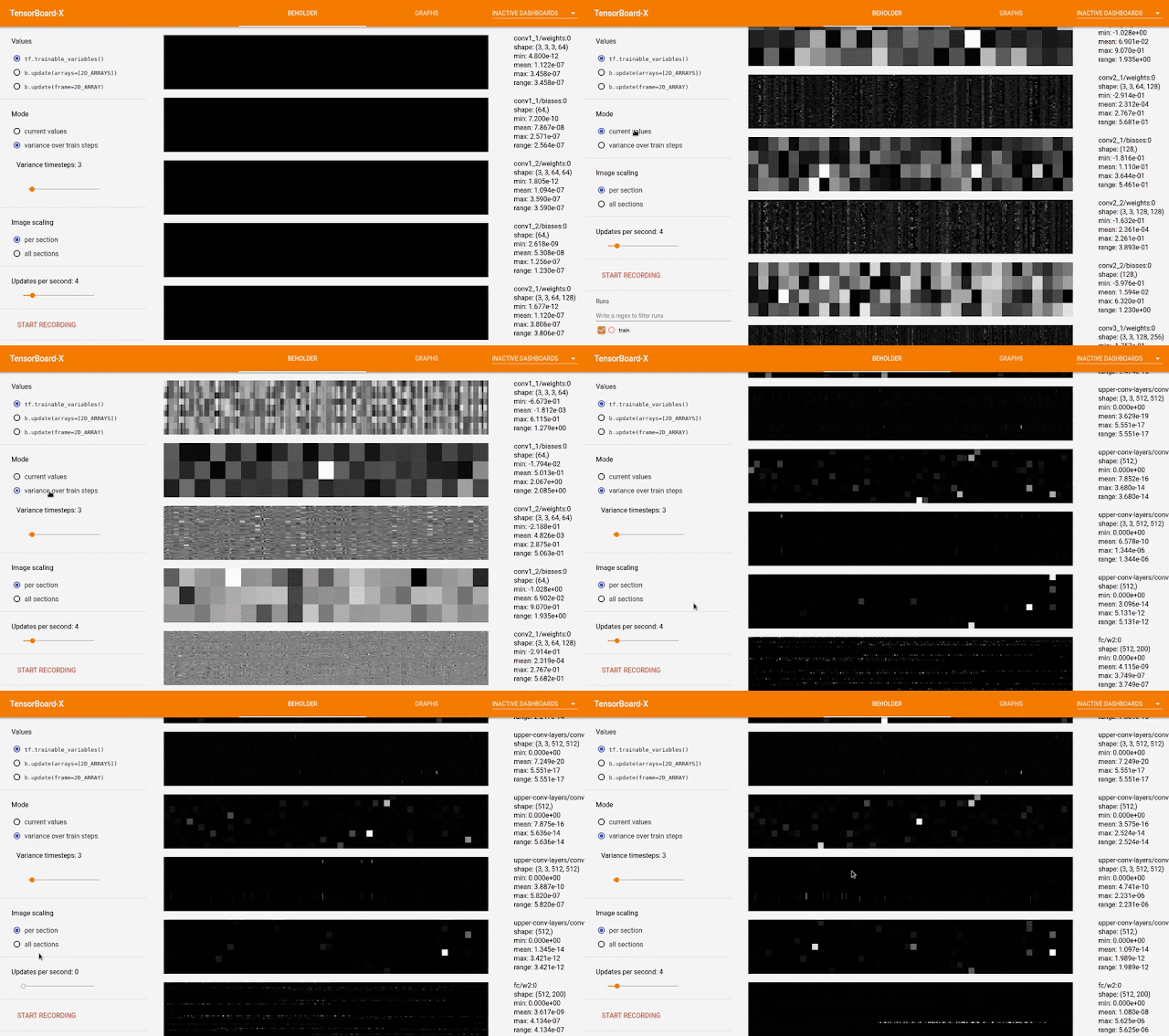
A notable example of how contributors are already using the TensorBoard API is Beholder, which was recently created by Chris Anderson while working on his master’s degree. Beholder shows a live video feed of data (e.g. gradients and convolution filters) as a model trains. You can watch the demo video here.
We look forward to seeing what innovations will come out of the community. If you plan to contribute a plugin to TensorBoard’s repository, you should get in touch with us first through the issue tracker with your idea so that we can help out and possibly guide you.

Acknowledgements
Dandelion Mané and William Chargin played crucial roles in building this API.


Launching the Speech Commands Dataset


At Google, we’re often asked how to get started using deep learning for speech and other audio recognition problems, like detecting keywords or commands. And while there are some great open source speech recognition systems like Kaldi that can use neural networks as a component, their sophistication makes them tough to use as a guide to a simpler tasks. Perhaps more importantly, there aren’t many free and openly available datasets ready to be used for a beginner’s tutorial (many require preprocessing before a neural network model can be built on them) or that are well suited for simple keyword detection.

To solve these problems, the TensorFlow and AIY teams have created the Speech Commands Dataset, and used it to add training* and inference sample code to TensorFlow. The dataset has 65,000 one-second long utterances of 30 short words, by thousands of different people, contributed by members of the public through the AIY website. It’s released under a Creative Commons BY 4.0 license, and will continue to grow in future releases as more contributions are received. The dataset is designed to let you build basic but useful voice interfaces for applications, with common words like “Yes”, “No”, digits, and directions included. The infrastructure we used to create the data has been open sourced too, and we hope to see it used by the wider community to create their own versions, especially to cover underserved languages and applications.

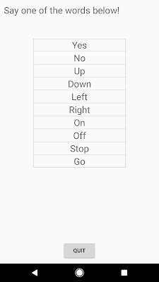
To try it out for yourself, download the prebuilt set of the TensorFlow Android demo applications and open up “TF Speech”. You’ll be asked for permission to access your microphone, and then see a list of ten words, each of which should light up as you say them.
The results will depend on whether your speech patterns are covered by the dataset, so it may not be perfect — commercial speech recognition systems are a lot more complex than this teaching example. But we’re hoping that as more accents and variations are added to the dataset, and as the community contributes improved models to TensorFlow, we’ll continue to see improvements and extensions.

You can also learn how to train your own version of this model through the new audio recognition tutorial on TensorFlow.org. With the latest development version of the framework and a modern desktop machine, you can download the dataset and train the model in just a few hours. You’ll also see a wide variety of options to customize the neural network for different problems, and to make different latency, size, and accuracy tradeoffs to run on different platforms.

We are excited to see what new applications people are able to build with the help of this dataset and tutorial, so I hope you get a chance to dive in and start recognizing!


* The architecture this network is based on is described in Convolutional Neural Networks for Small-footprint Keyword Spotting, presented at Interspeech 2015.

Teaching Robots to Understand Semantic Concepts


Machine learning can allow robots to acquire complex skills, such as grasping and opening doors. However, learning these skills requires us to manually program reward functions that the robots then attempt to optimize. In contrast, people can understand the goal of a task just from watching someone else do it, or simply by being told what the goal is. We can do this because we draw on our own prior knowledge about the world: when we see someone cut an apple, we understand that the goal is to produce two slices, regardless of what type of apple it is, or what kind of tool is used to cut it. Similarly, if we are told to pick up the apple, we understand which object we are to grab because we can ground the word “apple” in the environment: we know what it means.

These are semantic concepts: salient events like producing two slices, and object categories denoted by words such as “apple.” Can we teach robots to understand semantic concepts, to get them to follow simple commands specified through categorical labels or user-provided examples? In this post, we discuss some of our recent work on robotic learning that combines experience that is autonomously gathered by the robot, which is plentiful but lacks human-provided labels, with human-labeled data that allows a robot to understand semantics. We will describe how robots can use their experience to understand the salient events in a human-provided demonstration, mimic human movements despite the differences between human robot bodies, and understand semantic categories, like “toy” and “pen”, to pick up objects based on user commands.

Understanding human demonstrations with deep visual features
In the first set of experiments, which appear in our paper Unsupervised Perceptual Rewards for Imitation Learning, our is aim is to enable a robot to understand a task, such as opening a door, from seeing only a small number of unlabeled human demonstrations. By analyzing these demonstrations, the robot must understand what is the semantically salient event that constitutes task success, and then use reinforcement learning to perform it.
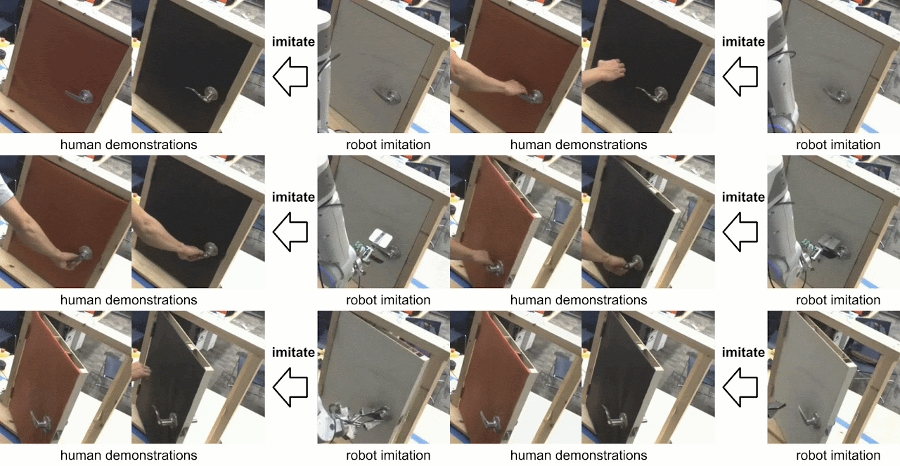
Examples of human demonstrations (left) and the corresponding robotic imitation (right).
Unsupervised learning on very small datasets is one of the most challenging scenarios in machine learning. To make this feasible, we use deep visual features from a large network trained for image recognition on ImageNet. Such features are known to be sensitive to semantic concepts, while maintaining invariance to nuisance variables such as appearance and lighting. We use these features to interpret user-provided demonstrations, and show that it is indeed possible to learn reward functions in an unsupervised fashion from a few demonstrations and without retraining.
Example of reward functions learned solely from observation for the door opening tasks. Rewards progressively increase from zero to the maximum reward as a task is completed.
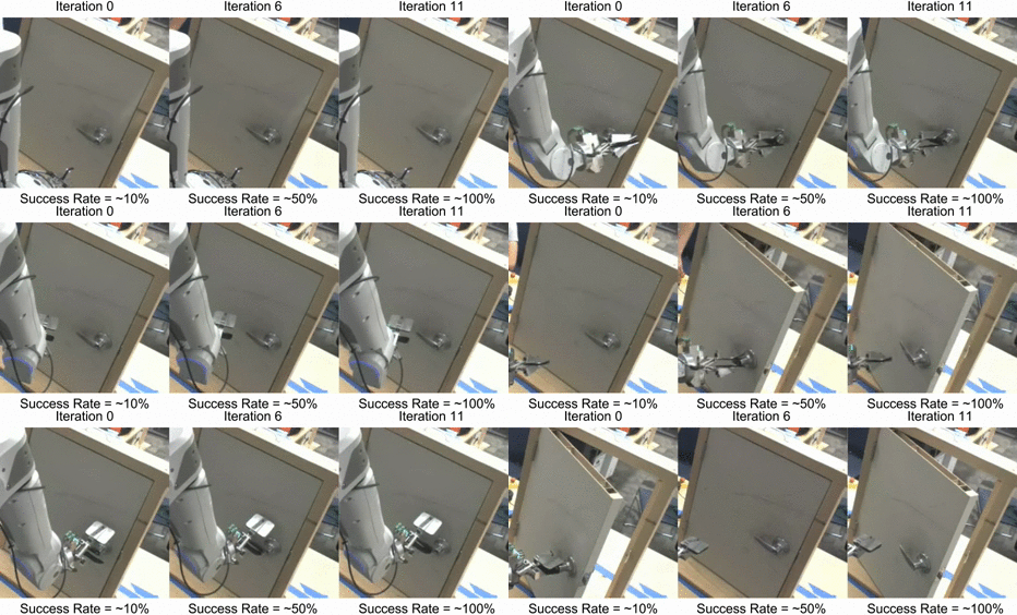
After learning a reward function from observation only, we use it to guide a robot to learn a door opening task, using only the images to evaluate the reward function. With the help of an initial kinesthetic demonstration that succeeds about 10% of the time, the robot learns to improve to 100% accuracy using the learned reward function.
Learning progression.
Emulating human movements with self-supervision and imitation.
In Time-Contrastive Networks: Self-Supervised Learning from Multi-View Observation, we propose a novel approach to learn about the world from observation and demonstrate it through self-supervised pose imitation. Our approach relies primarily on co-occurrence in time and space for supervision: by training to distinguish frames from different times of a video, it learns to disentangle and organize reality into useful abstract representations.

In a pose imitation task for example, different dimensions of the representation may encode for different joints of a human or robotic body. Rather than defining by hand a mapping between human and robot joints (which is ambiguous in the first place because of physiological differences), we let the robot learn to imitate in an end-to-end fashion. When our model is simultaneously trained on human and robot observations, it naturally discovers the correspondence between the two, even though no correspondence is provided. We thus obtain a robot that can imitate human poses without having ever been given a correspondence between humans and robots.
Self-supervised human pose imitation by a robot.
A striking evidence of the benefits of learning end-to-end is the many-to-one and highly non-linear joints mapping shown above. In this example, the up-down motion involves many joints for the human while only one joint is needed for the robot. We show that the robot has discovered this highly complex mapping on its own, without any explicit human pose information.

Grasping with semantic object categories
The experiments above illustrate how a person can specify a goal for a robot through an example demonstration, in which case the robots must interpret the semantics of the task -- salient events and relevant features of the pose. What if instead of showing the task, the human simply wants to tell it to what to do? This also requires the robot to understand semantics, in order to identify which objects in the world correspond to the semantic category specified by the user. In End-to-End Learning of Semantic Grasping, we study how a combination of manually labeled and autonomously collected data can be used to perform the task of semantic grasping, where the robot must pick up an object from a cluttered bin that matches a user-specified class label, such as “eraser” or “toy.”
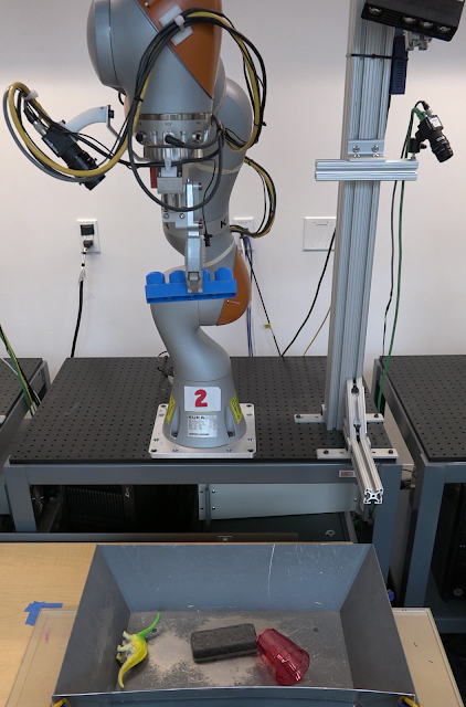
In our semantic grasping setup, the robotic arm is tasked with picking up an object corresponding to a user-provided semantic category (e.g. Legos).
To learn how to perform semantic grasping, our robots first gather a large dataset of grasping data by autonomously attempting to pick up a large variety of objects, as detailed in our previous post and prior work. This data by itself can allow a robot to pick up objects, but doesn’t allow it to understand how to associate them with semantic labels. To enable an understanding of semantics, we again enlist a modest amount of human supervision. Each time a robot successfully grasps an object, it presents it to the camera in a canonical pose, as illustrated below.
The robot presents objects to the camera after grasping. These images can be used to label which object category was picked up.
A subset of these images is then labeled by human labelers. Since the presentation images show the object in a canonical pose, it is easy to then propagate these labels to the remaining presentation images by training a classifier on the labeled examples. The labeled presentation images then tell the robot which object was actually picked up, and it can associate this label, in hindsight, with the images that it observed while picking up that object from the bin.

Using this labeled dataset, we can then train a two-stream model that predicts which object will be grasped, conditioned on the current image and the actions that the robot might take. The two-stream model that we employ is inspired by the dorsal-ventral decomposition observed in the human visual cortex, where the ventral stream reasons about the semantic class of objects, while the dorsal stream reasons about the geometry of the grasp. Crucially, the ventral stream can incorporate auxiliary data consisting of labeled images of objects (not necessarily from the robot), while the dorsal stream can incorporate auxiliary data of grasping that does not have semantic labels, allowing the entire system to be trained more effectively using larger amounts of heterogeneously labeled data. In this way, we can combine a limited amount of human labels with a large amount of autonomously collected robotic data to grasp objects based on desired semantic category, as illustrated in the video below:
Future Work
Our experiments show how limited semantically labeled data can be combined with data that is collected and labeled automatically by the robots, in order to enable robots to understand events, object categories, and user demonstrations. In the future, we might imagine that robotic systems could be trained with a combination of user-annotated data and ever-increasing autonomously collected datasets, improving robotic capability and easing the engineering burden of designing autonomous robots. Furthermore, as robotic systems collect more and more automatically annotated data in the real world, this data can be used to improve not just robotic systems, but also systems for computer vision, speech recognition, and natural language processing that can all benefit from such large auxiliary data sources.

Of course, we are not the first to consider the intersection of robotics and semantics. Extensive prior work in natural language understanding, robotic perception, grasping, and imitation learning has considered how semantics and action can be combined in a robotic system. However, the experiments we discussed above might point the way to future work into combining self-supervised and human-labeled data in the context of autonomous robotic systems.

Acknowledgements
The research described in this post was performed by Pierre Sermanet, Kelvin Xu, Corey Lynch, Jasmine Hsu, Eric Jang, Sudheendra Vijayanarasimhan, Peter Pastor, Julian Ibarz, and Sergey Levine. We also thank Mrinal Kalakrishnan, Ali Yahya, and Yevgen Chebotar for developing the policy learning framework used for the door task, and John-Michael Burke for conducting experiments for semantic grasping.

Unsupervised Perceptual Rewards for Imitation Learning was presented at RSS 2017 by Kelvin Xu, and Time-Contrastive Networks: Self-Supervised Learning from Multi-View Observation will be presented this week at the CVPR Workshop on Deep Learning for Robotic Vision.

Building Your Own Neural Machine Translation System in TensorFlow


Machine translation – the task of automatically translating between languages – is one of the most active research areas in the machine learning community. Among the many approaches to machine translation, sequence-to-sequence ("seq2seq") models [1, 2] have recently enjoyed great success and have become the de facto standard in most commercial translation systems, such as Google Translate, thanks to its ability to use deep neural networks to capture sentence meanings. However, while there is an abundance of material on seq2seq models such as OpenNMT or tf-seq2seq, there is a lack of material that teaches people both the knowledge and the skills to easily build high-quality translation systems.

Today we are happy to announce a new Neural Machine Translation (NMT) tutorial for TensorFlow that gives readers a full understanding of seq2seq models and shows how to build a competitive translation model from scratch. The tutorial is aimed at making the process as simple as possible, starting with some background knowledge on NMT and walking through code details to build a vanilla system. It then dives into the attention mechanism [3, 4], a key ingredient that allows NMT systems to handle long sentences. Finally, the tutorial provides details on how to replicate key features in the Google’s NMT (GNMT) system [5] to train on multiple GPUs.

The tutorial also contains detailed benchmark results, which users can replicate on their own. Our models provide a strong open-source baseline with performance on par with GNMT results [5]. We achieve 24.4 BLEU points on the popular WMT’14 English-German translation task.
Other benchmark results (English-Vietnamese, German-English) can be found in the tutorial.

In addition, this tutorial showcases the fully dynamic seq2seq API (released with TensorFlow 1.2) aimed at making building seq2seq models clean and easy:
  • Easily read and preprocess dynamically sized input sequences using the new input pipeline in tf.contrib.data.
  • Use padded batching and sequence length bucketing to improve training and inference speeds.
  • Train seq2seq models using popular architectures and training schedules, including several types of attention and scheduled sampling.
  • Perform inference in seq2seq models using in-graph beam search.
  • Optimize seq2seq models for multi-GPU settings.
We hope this will help spur the creation of, and experimentation with, many new NMT models by the research community. To get started on your own research, check out the tutorial on GitHub!

Core contributors
Thang Luong, Eugene Brevdo, and Rui Zhao.

Acknowledgements
We would like to especially thank our collaborator on the NMT project, Rui Zhao. Without his tireless effort, this tutorial would not have been possible. Additional thanks go to Denny Britz, Anna Goldie, Derek Murray, and Cinjon Resnick for their work bringing new features to TensorFlow and the seq2seq library. Lastly, we thank Lukasz Kaiser for the initial help on the seq2seq codebase; Quoc Le for the suggestion to replicate GNMT; Yonghui Wu and Zhifeng Chen for details on the GNMT systems; as well as the Google Brain team for their support and feedback!

References
[1] Sequence to sequence learning with neural networks, Ilya Sutskever, Oriol Vinyals, and Quoc V. Le. NIPS, 2014.
[2] Learning phrase representations using RNN encoder-decoder for statistical machine translation, Kyunghyun Cho, Bart Van Merrienboer, Caglar Gulcehre, Dzmitry Bahdanau, Fethi Bougares, Holger Schwenk, and Yoshua Bengio. EMNLP 2014.
[3] Neural machine translation by jointly learning to align and translate, Dzmitry Bahdanau, Kyunghyun Cho, and Yoshua Bengio. ICLR, 2015.
[4] Effective approaches to attention-based neural machine translation, Minh-Thang Luong, Hieu Pham, and Christopher D Manning. EMNLP, 2015.
[5] Google’s Neural Machine Translation System: Bridging the Gap between Human and Machine Translation, Yonghui Wu, Mike Schuster, Zhifeng Chen, Quoc V. Le, Mohammad Norouzi, Wolfgang Macherey, Maxim Krikun, Yuan Cao, Qin Gao, Klaus Macherey, Jeff Klingner, Apurva Shah, Melvin Johnson, Xiaobing Liu, Łukasz Kaiser, Stephan Gouws, Yoshikiyo Kato, Taku Kudo, Hideto Kazawa, Keith Stevens, George Kurian, Nishant Patil, Wei Wang, Cliff Young, Jason Smith, Jason Riesa, Alex Rudnick, Oriol Vinyals, Greg Corrado, Macduff Hughes, Jeffrey Dean. Technical Report, 2016.

The Google Brain Residency Program — One Year Later


“Coming from a background in statistics, physics, and chemistry, the Google Brain Residency was my first exposure to both deep learning and serious programming. I enjoyed the autonomy that I was given to research diverse topics of my choosing: deep learning for computer vision and language, reinforcement learning, and theory. I originally intended to pursue a statistics PhD but my experience here spurred me to enroll in the Stanford CS program starting this fall!”
- Melody Guan, 2016 Google Brain Residency Alumna

This month marks the end of an incredibly successful year for our first class of the Google Brain Residency Program. This one-year program was created as an opportunity for individuals from diverse educational backgrounds and experiences to dive into research in machine learning and deep learning. Over the past year, the Residents familiarized themselves with the literature, designed and implemented experiments at Google scale, and engaged in cutting edge research in a wide variety of subjects ranging from theory to robotics to music generation.

To date, the inaugural class of Residents have published over 30 papers at leading machine learning publication venues such as ICLR (15), ICML (11), CVPR (3), EMNLP (2), RSS, GECCO, ISMIR, ISMB and Cosyne. An additional 18 papers are currently under review at NIPS, ICCV, BMVC and Nature Methods. Two of the above papers were published in Distill, exploring how deconvolution causes checkerboard artifacts and presenting ways of visualizing a generative model of handwriting.
A Distill article by residents interactively explores how a neural network generates handwriting.
A system that explores how robots can learn to imitate human motion from observation. For more details, see “Time-Contrastive Networks: Self-Supervised Learning from Multi-View Observation” (Co-authored by Resident Corey Lynch, along with P. Sermanet, , J. Hsu, S. Levine, accepted to CVPR Workshop 2017)
A model that uses reinforcement learning to train distributed deep learning networks at large scale by optimizing computations to hardware devices assignment. For more details, see “Device Placement Optimization with Reinforcement Learning” (Co-authored by Residents Azalia Mirhoseini and Hieu Pham, along with Q. Le, B. Steiner, R. Larsen, Y. Zhou, N. Kumar, M. Norouzi, S. Bengio, J. Dean, submitted to ICML 2017).
An approach to automate the process of discovering optimization methods, with a focus on deep learning architectures. Final version of the paper “Neural Optimizer Search with Reinforcement Learning” (Co-authored by Residents Irwan Bello and Barret Zoph, along with V. Vasudevan, Q. Le, submitted to ICML 2017) coming soon.
Residents have also made significant contributions to the open source community with general-purpose sequence-to-sequence models (used for example in translation), music synthesis, mimicking human sketching, subsampling a sequence for model training, an efficient “attention” mechanism for models, and time series analysis (particularly for neuroscience).

The end of the program year marks our Residents embarking on the next stages in their careers. Many are continuing their research careers on the Google Brain team as full time employees. Others have chosen to enter top machine learning Ph.D. programs at schools such as Stanford University, UC Berkeley, Cornell University, Oxford University and NYU, University of Toronto and CMU. We could not be more proud to see where their hard work and experiences will take them next!

As we “graduate” our first class, this week we welcome our next class of 35 incredibly talented Residents who have joined us from a wide range of experience and education backgrounds. We can’t wait to see how they will build on the successes of our first class and continue to push the team in new and exciting directions. We look forward to another exciting year of research and innovation ahead of us!

Applications to the 2018 Residency program will open in September 2017. To learn more about the program, visit g.co/brainresidency.

MultiModel: Multi-Task Machine Learning Across Domains


Over the last decade, the application and performance of Deep Learning has progressed at an astonishing rate. However, the current state of the field is that the neural network architectures are highly specialized to specific domains of application. An important question remains unanswered: Will a convergence between these domains facilitate a unified model capable of performing well across multiple domains?

Today, we present MultiModel, a neural network architecture that draws from the success of vision, language and audio networks to simultaneously solve a number of problems spanning multiple domains, including image recognition, translation and speech recognition. While strides have been made in this direction before, namely in Google’s Multilingual Neural Machine Translation System used in Google Translate, MultiModel is a first step towards the convergence of vision, audio and language understanding into a single network.

The inspiration for how MultiModel handles multiple domains comes from how the brain transforms sensory input from different modalities (such as sound, vision or taste), into a single shared representation and back out in the form of language or actions. As an analog to these modalities and the transformations they perform, MultiModel has a number of small modality-specific sub-networks for audio, images, or text, and a shared model consisting of an encoder, input/output mixer and decoder, as illustrated below.
MultiModel architecture: small modality-specific sub-networks work with a shared encoder, I/O mixer and decoder. Each petal represents a modality, transforming to and from the internal representation.
We demonstrate that MultiModel is capable of learning eight different tasks simultaneously: it can detect objects in images, provide captions, recognize speech, translate between four pairs of languages, and do grammatical constituency parsing at the same time. The input is given to the model together with a very simple signal that determines which output we are requesting. Below we illustrate a few examples taken from a MultiModel trained jointly on these eight tasks1:
When designing MultiModel it became clear that certain elements from each domain of research (vision, language and audio) were integral to the model’s success in related tasks. We demonstrate that these computational primitives (such as convolutions, attention, or mixture-of-experts layers) clearly improve performance on their originally intended domain of application, while not hindering MultiModel’s performance on other tasks. It is not only possible to achieve good performance while training jointly on multiple tasks, but on tasks with limited quantities of data, the performance actually improves. To our surprise, this happens even if the tasks come from different domains that would appear to have little in common, e.g., an image recognition task can improve performance on a language task.

It is important to note that while MultiModel does not establish new performance records, it does provide insight into the dynamics of multi-domain multi-task learning in neural networks, and the potential for improved learning on data-limited tasks by the introduction of auxiliary tasks. There is a longstanding saying in machine learning: “the best regularizer is more data”; in MultiModel, this data can be sourced across domains, and consequently can be obtained more easily than previously thought. MultiModel provides evidence that training in concert with other tasks can lead to good results and improve performance on data-limited tasks.

Many questions about multi-domain machine learning remain to be studied, and we will continue to work on tuning Multimodel and improving its performance. To allow this research to progress quickly, we open-sourced MultiModel as part of the Tensor2Tensor library. We believe that such synergetic models trained on data from multiple domains will be the next step in deep learning and will ultimately solve tasks beyond the reach of current narrowly trained networks.

Acknowledgements
This work is a collaboration between Googlers Łukasz Kaiser, Noam Shazeer, Ashish Vaswani, Niki Parmar, Llion Jones and Jakob Uszkoreit, and Aidan N. Gomez from the University of Toronto. It was performed while Aidan was working with the Google Brain team.


1 The 8 tasks were: (1) speech recognition (WSJ corpus), (2) image classification (ImageNet), (3) image captioning (MS COCO), (4) parsing (Penn Treebank), (5) English-German translation, (6) German-English translation, (7) English-French translation, (8) French-English translation (all using WMT data-sets).

Accelerating Deep Learning Research with the Tensor2Tensor Library


Deep Learning (DL) has enabled the rapid advancement of many useful technologies, such as machine translation, speech recognition and object detection. In the research community, one can find code open-sourced by the authors to help in replicating their results and further advancing deep learning. However, most of these DL systems use unique setups that require significant engineering effort and may only work for a specific problem or architecture, making it hard to run new experiments and compare the results.

Today, we are happy to release Tensor2Tensor (T2T), an open-source system for training deep learning models in TensorFlow. T2T facilitates the creation of state-of-the art models for a wide variety of ML applications, such as translation, parsing, image captioning and more, enabling the exploration of various ideas much faster than previously possible. This release also includes a library of datasets and models, including the best models from a few recent papers (Attention Is All You Need, Depthwise Separable Convolutions for Neural Machine Translation and One Model to Learn Them All) to help kick-start your own DL research.

Translation Model
Training time
BLEU (difference from baseline)
Transformer (T2T)
3 days on 8 GPU
28.4 (+7.8)
SliceNet (T2T)
6 days on 32 GPUs
26.1 (+5.5)
1 day on 64 GPUs
26.0 (+5.4)
ConvS2S
18 days on 1 GPU
25.1 (+4.5)
GNMT
1 day on 96 GPUs
24.6 (+4.0)
8 days on 32 GPUs
23.8 (+3.2)
MOSES (phrase-based baseline)
N/A
20.6 (+0.0)
BLEU scores (higher is better) on the standard WMT English-German translation task.
As an example of the kind of improvements T2T can offer, we applied the library to machine translation. As you can see in the table above, two different T2T models, SliceNet and Transformer, outperform the previous state-of-the-art, GNMT+MoE. Our best T2T model, Transformer, is 3.8 points better than the standard GNMT model, which itself was 4 points above the baseline phrase-based translation system, MOSES. Notably, with T2T you can approach previous state-of-the-art results with a single GPU in one day: a small Transformer model (not shown above) gets 24.9 BLEU after 1 day of training on a single GPU. Now everyone with a GPU can tinker with great translation models on their own: our github repo has instructions on how to do that.

Modular Multi-Task Training
The T2T library is built with familiar TensorFlow tools and defines multiple pieces needed in a deep learning system: data-sets, model architectures, optimizers, learning rate decay schemes, hyperparameters, and so on. Crucially, it enforces a standard interface between all these parts and implements current ML best practices. So you can pick any data-set, model, optimizer and set of hyperparameters, and run the training to check how it performs. We made the architecture modular, so every piece between the input data and the predicted output is a tensor-to-tensor function. If you have a new idea for the model architecture, you don’t need to replace the whole setup. You can keep the embedding part and the loss and everything else, just replace the model body by your own function that takes a tensor as input and returns a tensor.

This means that T2T is flexible, with training no longer pinned to a specific model or dataset. It is so easy that even architectures like the famous LSTM sequence-to-sequence model can be defined in a few dozen lines of code. One can also train a single model on multiple tasks from different domains. Taken to the limit, you can even train a single model on all data-sets concurrently, and we are happy to report that our MultiModel, trained like this and included in T2T, yields good results on many tasks even when training jointly on ImageNet (image classification), MS COCO (image captioning), WSJ (speech recognition), WMT (translation) and the Penn Treebank parsing corpus. It is the first time a single model has been demonstrated to be able to perform all these tasks at once.

Built-in Best Practices
With this initial release, we also provide scripts to generate a number of data-sets widely used in the research community1, a handful of models2, a number of hyperparameter configurations, and a well-performing implementation of other important tricks of the trade. While it is hard to list them all, if you decide to run your model with T2T you’ll get for free the correct padding of sequences and the corresponding cross-entropy loss, well-tuned parameters for the Adam optimizer, adaptive batching, synchronous distributed training, well-tuned data augmentation for images, label smoothing, and a number of hyper-parameter configurations that worked very well for us, including the ones mentioned above that achieve the state-of-the-art results on translation and may help you get good results too.

As an example, consider the task of parsing English sentences into their grammatical constituency trees. This problem has been studied for decades and competitive methods were developed with a lot of effort. It can be presented as a sequence-to-sequence problem and be solved with neural networks, but it used to require a lot of tuning. With T2T, it took us only a few days to add the parsing data-set generator and adjust our attention transformer model to train on this problem. To our pleasant surprise, we got very good results in only a week:

Parsing Model
F1 score (higher is better)
Transformer (T2T)
91.3
Dyer et al.
91.7
Zhu et al.
90.4
Socher et al.
90.4
Vinyals & Kaiser et al.
88.3
Parsing F1 scores on the standard test set, section 23 of the WSJ. We only compare here models trained discriminatively on the Penn Treebank WSJ training set, see the paper for more results.

Contribute to Tensor2Tensor
In addition to exploring existing models and data-sets, you can easily define your own model and add your own data-sets to Tensor2Tensor. We believe the already included models will perform very well for many NLP tasks, so just adding your data-set might lead to interesting results. By making T2T modular, we also make it very easy to contribute your own model and see how it performs on various tasks. In this way the whole community can benefit from a library of baselines and deep learning research can accelerate. So head to our github repository, try the new models, and contribute your own!

Acknowledgements
The release of Tensor2Tensor was only possible thanks to the widespread collaboration of many engineers and researchers. We want to acknowledge here the core team who contributed (in alphabetical order): Samy Bengio, Eugene Brevdo, Francois Chollet, Aidan N. Gomez, Stephan Gouws, Llion Jones, Łukasz Kaiser, Nal Kalchbrenner, Niki Parmar, Ryan Sepassi, Noam Shazeer, Jakob Uszkoreit, Ashish Vaswani.


1 We include a number of datasets for image classification (MNIST, CIFAR-10, CIFAR-100, ImageNet), image captioning (MS COCO), translation (WMT with multiple languages including English-German and English-French), language modelling (LM1B), parsing (Penn Treebank), natural language inference (SNLI), speech recognition (TIMIT), algorithmic problems (over a dozen tasks from reversing through addition and multiplication to algebra) and we will be adding more and welcome your data-sets too.

2 Including LSTM sequence-to-sequence RNNs, convolutional networks also with separable convolutions (e.g., Xception), recently researched models like ByteNet or the Neural GPU, and our new state-of-the-art models mentioned in this post that we will be actively updating in the repository.


Using Machine Learning to Explore Neural Network Architecture


At Google, we have successfully applied deep learning models to many applications, from image recognition to speech recognition to machine translation. Typically, our machine learning models are painstakingly designed by a team of engineers and scientists. This process of manually designing machine learning models is difficult because the search space of all possible models can be combinatorially large — a typical 10-layer network can have ~1010 candidate networks! For this reason, the process of designing networks often takes a significant amount of time and experimentation by those with significant machine learning expertise.
Our GoogleNet architecture. Design of this network required many years of careful experimentation and refinement from initial versions of convolutional architectures.
To make this process of designing machine learning models much more accessible, we’ve been exploring ways to automate the design of machine learning models. Among many algorithms we’ve studied, evolutionary algorithms [1] and reinforcement learning algorithms [2] have shown great promise. But in this blog post, we’ll focus on our reinforcement learning approach and the early results we’ve gotten so far.

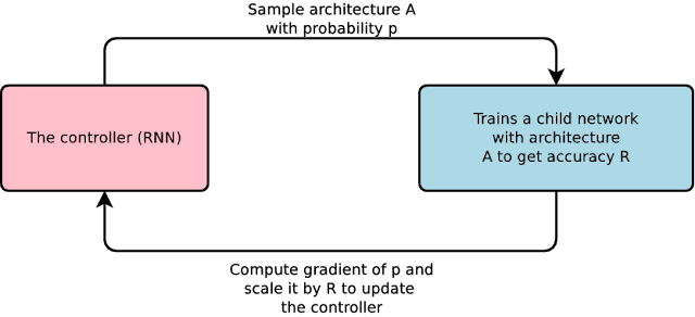
In our approach (which we call "AutoML"), a controller neural net can propose a “child” model architecture, which can then be trained and evaluated for quality on a particular task. That feedback is then used to inform the controller how to improve its proposals for the next round. We repeat this process thousands of times — generating new architectures, testing them, and giving that feedback to the controller to learn from. Eventually the controller learns to assign high probability to areas of architecture space that achieve better accuracy on a held-out validation dataset, and low probability to areas of architecture space that score poorly. Here’s what the process looks like:
We’ve applied this approach to two heavily benchmarked datasets in deep learning: image recognition with CIFAR-10 and language modeling with Penn Treebank. On both datasets, our approach can design models that achieve accuracies on par with state-of-art models designed by machine learning experts (including some on our own team!).

So, what kind of neural nets does it produce? Let’s take one example: a recurrent architecture that’s trained to predict the next word on the Penn Treebank dataset. On the left here is a neural net designed by human experts. On the right is a recurrent architecture created by our method:

The machine-chosen architecture does share some common features with the human design, such as using addition to combine input and previous hidden states. However, there are some notable new elements — for example, the machine-chosen architecture incorporates a multiplicative combination (the left-most blue node on the right diagram labeled “elem_mult”). This type of combination is not common for recurrent networks, perhaps because researchers see no obvious benefit for having it. Interestingly, a simpler form of this approach was recently suggested by human designers, who also argued that this multiplicative combination can actually alleviate gradient vanishing/exploding issues, suggesting that the machine-chosen architecture was able to discover a useful new neural net architecture.

This approach may also teach us something about why certain types of neural nets work so well. The architecture on the right here has many channels so that the gradient can flow backwards, which may help explain why LSTM RNNs work better than standard RNNs.

Going forward, we’ll work on careful analysis and testing of these machine-generated architectures to help refine our understanding of them. If we succeed, we think this can inspire new types of neural nets and make it possible for non-experts to create neural nets tailored to their particular needs, allowing machine learning to have a greater impact to everyone.

References

[1] Large-Scale Evolution of Image Classifiers, Esteban Real, Sherry Moore, Andrew Selle, Saurabh Saxena, Yutaka Leon Suematsu, Quoc Le, Alex Kurakin. International Conference on Machine Learning, 2017.

[2] Neural Architecture Search with Reinforcement Learning, Barret Zoph, Quoc V. Le. International Conference on Learning Representations, 2017.