Welcome to Part 3 of a blog series that introduces TensorFlow Datasets and Estimators. Part 1 focused on pre-made Estimators, while Part 2 discussed feature columns. Here in Part 3, you'll learn how to create your own custom Estimators. In particular, we're going to demonstrate how to create a custom Estimator that mimics DNNClassifier's behavior when solving the Iris problem.

If you are feeling impatient, feel free to compare and contrast the following full programs:

• Source code for Iris implemented with the pre-made DNNClassifier Estimator here.
• Source code for Iris implemented with the custom Estimator here.

Pre-made vs. custom

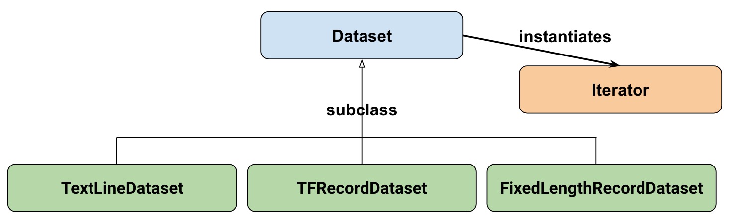
As Figure 1 shows, pre-made Estimators are subclasses of the tf.estimator.Estimatorbase class, while custom Estimators are an instantiation of tf.estimator.Estimator:

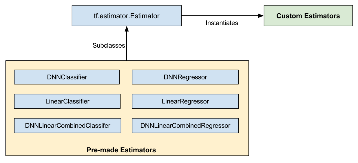
Figure 1. Pre-made and custom Estimators are all Estimators.

Pre-made Estimators are fully-baked. Sometimes though, you need more control over an Estimator's behavior. That's where custom Estimators come in.

You can create a custom Estimator to do just about anything. If you want hidden layers connected in some unusual fashion, write a custom Estimator. If you want to calculate a unique metric for your model, write a custom Estimator. Basically, if you want an Estimator optimized for your specific problem, write a custom Estimator.

A model function (model_fn) implements your model. The only difference between working with pre-made Estimators and custom Estimators is:

• With pre-made Estimators, someone already wrote the model function for you.
• With custom Estimators, you must write the model function.

Your model function could implement a wide range of algorithms, defining all sorts of hidden layers and metrics. Like input functions, all model functions must accept a standard group of input parameters and return a standard group of output values. Just as input functions can leverage the Dataset API, model functions can leverage the Layers API and the Metrics API.

Iris as a pre-made Estimator: A quick refresher

Before demonstrating how to implement Iris as a custom Estimator, we wanted to remind you how we implemented Iris as a pre-made Estimator in Part 1 of this series. In that Part, we created a fully connected, deepneural network for the Iris dataset simply by instantiating a pre-made Estimator as follows:

# Instantiate a deep neural network classifier.
classifier = tf.estimator.DNNClassifier(
   feature_columns=feature_columns, # The input features to our model.
   hidden_units=[10, 10], # Two layers, each with 10 neurons.
   n_classes=3, # The number of output classes (three Iris species).
   model_dir=PATH) # Pathname of directory where checkpoints, etc. are stored.

The preceding code creates a deep neural network with the following characteristics:

• A list of feature columns. (The definitions of the feature columns are not shown in the preceding snippet.) For Iris, the feature columns are numeric representations of four input features.
• Two fully connected layers, each having 10 neurons. A fully connected layer (also called a dense layer) is connected to every neuron in the subsequent layer.
• An output layer consisting of a three-element list. The elements of that list are all floating-point values; the sum of those values must be 1.0 (this is a probability distribution).
• A directory (PATH) in which the trained model and various checkpoints will be stored.

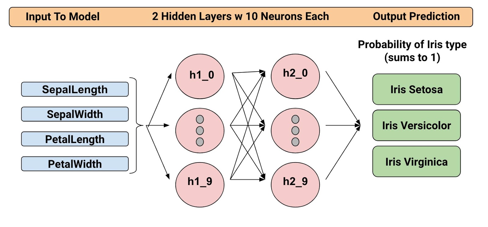
Figure 2 illustrates the input layer, hidden layers, and output layer of the Iris model. For reasons pertaining to clarity, we've only drawn 4 of the nodes in each hidden layer.

Figure 2. Our implementation of Iris contains four features, two hidden layers, and a logits output layer.

Let's see how to solve the same Iris problem with a custom Estimator.

Input function

One of the biggest advantages of the Estimator framework is that you can experiment with different algorithms without changing your data pipeline. We will therefore reuse much of the input function from Part 1:

def my_input_fn(file_path, repeat_count=1, shuffle_count=1):
   def decode_csv(line):
       parsed_line = tf.decode_csv(line, [[0.], [0.], [0.], [0.], [0]])
       label = parsed_line[-1]  # Last element is the label
       del parsed_line[-1]  # Delete last element
       features = parsed_line  # Everything but last elements are the features
       d = dict(zip(feature_names, features)), label
       return d

   dataset = (tf.data.TextLineDataset(file_path)  # Read text file
       .skip(1)  # Skip header row
       .map(decode_csv, num_parallel_calls=4)  # Decode each line
       .cache() # Warning: Caches entire dataset, can cause out of memory
       .shuffle(shuffle_count)  # Randomize elems (1 == no operation)
       .repeat(repeat_count)    # Repeats dataset this # times
       .batch(32)
       .prefetch(1)  # Make sure you always have 1 batch ready to serve
   )
   iterator = dataset.make_one_shot_iterator()
   batch_features, batch_labels = iterator.get_next()
   return batch_features, batch_labels

Notice that the input function returns the following two values:

• batch_features, which is a dictionary. The dictionary's keys are the names of the features, and the dictionary's values are the feature's values.
• batch_labels, which is a list of the label's values for a batch.

Refer to Part 1 for full details on input functions.

Create feature columns

As detailed in Part 2 of our series, you must define your model's feature columns to specify the representation of each feature. Whether working with pre-made Estimators or custom Estimators, you define feature columns in the same fashion. For example, the following code creates feature columns representing the four features (all numerical) in the Iris dataset:

feature_columns = [
   tf.feature_column.numeric_column(feature_names[0]),
   tf.feature_column.numeric_column(feature_names[1]),
   tf.feature_column.numeric_column(feature_names[2]),
   tf.feature_column.numeric_column(feature_names[3])
]

Write a model function

We are now ready to write the model_fn for our custom Estimator. Let's start with the function declaration:

def my_model_fn(
   features, # This is batch_features from input_fn
   labels,   # This is batch_labels from input_fn
   mode):    # Instance of tf.estimator.ModeKeys, see below

The first two arguments are the features and labels returned from the input function; that is, features and labels are the handles to the data your model will use. The mode argument indicates whether the caller is requesting training, predicting, or evaluating.

To implement a typical model function, you must do the following:

• Define the model's layers.
• Specify the model's behavior in three the different modes.

Define the model's layers

If your custom Estimator generates a deep neural network, you must define the following three layers:

• an input layer
• one or more hidden layers
• an output layer

Use the Layers API (tf.layers) to define hidden and output layers.

If your custom Estimator generates a linear model, then you only have to generate a single layer, which we'll describe in the next section.

Define the input layer

Call tf.feature_column.input_layerto define the input layer for a deep neural network. For example:

# Create the layer of input
input_layer = tf.feature_column.input_layer(features, feature_columns)

The preceding line creates our input layer, reading our featuresthrough the input function and filtering them through the feature_columns defined earlier. See Part 2 for details on various ways to represent data through feature columns.

To create the input layer for a linear model, call tf.feature_column.linear_modelinstead of tf.feature_column.input_layer. Since a linear model has no hidden layers, the returned value from tf.feature_column.linear_model serves as both the input layer and output layer. In other words, the returned value from this function isthe prediction.

Establish Hidden Layers

If you are creating a deep neural network, you must define one or more hidden layers. The Layers API provides a rich set of functions to define all types of hidden layers, including convolutional, pooling, and dropout layers. For Iris, we're simply going to call tf.layers.Densetwice to create two dense hidden layers, each with 10 neurons. By "dense," we mean that each neuron in the first hidden layer is connected to each neuron in the second hidden layer. Here's the relevant code:

# Definition of hidden layer: h1
# (Dense returns a Callable so we can provide input_layer as argument to it)
h1 = tf.layers.Dense(10, activation=tf.nn.relu)(input_layer)

# Definition of hidden layer: h2
# (Dense returns a Callable so we can provide h1 as argument to it)
h2 = tf.layers.Dense(10, activation=tf.nn.relu)(h1)

The inputs parameter to tf.layers.Dense identifies the preceding layer. The layer preceding h1 is the input layer.

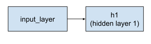
Figure 3. The input layer feeds into hidden layer 1.

The preceding layer to h2 is h1. So, the string of layers now looks like this:

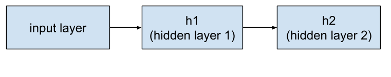
Figure 4. Hidden layer 1 feeds into hidden layer 2.

The first argument to tf.layers.Densedefines the number of its output neurons—10 in this case.

The activation parameter defines the activation function—Relu in this case.

Note that tf.layers.Denseprovides many additional capabilities, including the ability to set a multitude of regularization parameters. For the sake of simplicity, though, we're going to simply accept the default values of the other parameters. Also, when looking at tf.layersyou may encounter lower-case versions (e.g. tf.layers.dense). As a general rule, you should use the class versions which start with a capital letter (tf.layers.Dense).

Output Layer

We'll define the output layer by calling tf.layers.Dense yet again:

# Output 'logits' layer is three numbers = probability distribution
# (Dense returns a Callable so we can provide h2 as argument to it)
logits = tf.layers.Dense(3)(h2)

Notice that the output layer receives its input from h2. Therefore, the full set of layers is now connected as follows:

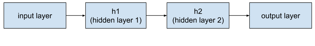
Figure 5. Hidden layer 2 feeds into the output layer.

When defining an output layer, the units parameter specifies the number of possible output values. So, by setting units to 3, the tf.layers.Densefunction establishes a three-element logits vector. Each cell of the logits vector contains the probability of the Iris being Setosa, Versicolor, or Virginica, respectively.

Since the output layer is a final layer, the call to tf.layers.Denseomits the optional activation parameter.

Implement training, evaluation, and prediction

The final step in creating a model function is to write branching code that implements prediction, evaluation, and training.

The model function gets invoked whenever someone calls the Estimator's train, evaluate, or predict methods. Recall that the signature for the model function looks like this:

def my_model_fn(
   features, # This is batch_features from input_fn
   labels,   # This is batch_labels from input_fn
   mode):    # Instance of tf.estimator.ModeKeys, see below

Focus on that third argument, mode. As the following table shows, when someone calls train, evaluate, or predict, the Estimator framework invokes your model function with the mode parameter set as follows:

Table 2. Values of mode.

For example, suppose you instantiate a custom Estimator to generate an object named classifier. Then, you might make the following call (never mind the parameters to my_input_fn at this time):

classifier.train(
  input_fn=lambda: my_input_fn(FILE_TRAIN, repeat_count=500, shuffle_count=256))

The Estimator framework then calls your model function with mode set to ModeKeys.TRAIN.

Your model function must provide code to handle all three of the mode values. For each mode value, your code must return an instance of tf.estimator.EstimatorSpec, which contains the information the caller requires. Let's examine each mode.

PREDICT

When model_fn is called with mode == ModeKeys.PREDICT, the model function must return a tf.estimator.EstimatorSpeccontaining the following information:

• the mode, which is tf.estimator.ModeKeys.PREDICT
• the prediction

The model must have been trained prior to making a prediction. The trained model is stored on disk in the directory established when you instantiated the Estimator.

For our case, the code to generate the prediction looks as follows:

# class_ids will be the model prediction for the class (Iris flower type)
# The output node with the highest value is our prediction
predictions = { 'class_ids': tf.argmax(input=logits, axis=1) }

# Return our prediction
if mode == tf.estimator.ModeKeys.PREDICT:
   return tf.estimator.EstimatorSpec(mode, predictions=predictions)

The block is surprisingly brief--the lines of code are simply the bucket at the end of a long hose that catches the falling predictions. After all, the Estimator has already done all the heavy lifting to make a prediction:

1. The input function provides the model function with data (feature values) to infer from.
2. The model function transforms those feature values into feature columns.
3. The model function runs those feature columns through the previously-trained model.

The output layer is a logits vector that contains the value of each of the three Iris species being the input flower. The tf.argmaxmethod selects the Iris species in that logits vector with the highest value.

Notice that the highest value is assigned to a dictionary key named class_ids. We return that dictionary through the predictions parameter of tf.estimator.EstimatorSpec. The caller can then retrieve the prediction by examining the dictionary passed back to the Estimator's predict method.

EVAL

When model_fn is called with mode == ModeKeys.EVAL, the model function must evaluate the model, returning loss and possibly one or more metrics.

We can calculate loss by calling tf.losses.sparse_softmax_cross_entropy. Here's the complete code:

# To calculate the loss, we need to convert our labels
# Our input labels have shape: [batch_size, 1]
labels = tf.squeeze(labels, 1)          # Convert to shape [batch_size]
loss = tf.losses.sparse_softmax_cross_entropy(labels=labels, logits=logits)

Now let's turn our attention to metrics. Although returning metrics is optional, most custom Estimators return at least one metric. TensorFlow provides a Metrics API (tf.metrics) to calculate different kinds of metrics. For brevity's sake, we'll only return accuracy. The tf.metrics.accuracycompares our predictions against the "true labels", that is, against the labels provided by the input function. The tf.metrics.accuracyfunction requires the labels and predictions to have the same shape (which we did earlier). Here's the call to tf.metrics.accuracy:

# Calculate the accuracy between the true labels, and our predictions
accuracy = tf.metrics.accuracy(labels, predictions['class_ids'])

When the model is called with mode == ModeKeys.EVAL, the model function returns a tf.estimator.EstimatorSpec containing the following information:

• the mode, which is tf.estimator.ModeKeys.EVAL
• the model's loss
• typically, one or more metrics encased in a dictionary.

So, we'll create a dictionary containing our sole metric (my_accuracy). If we had calculated other metrics, we would have added them as additional key/value pairs to that same dictionary. Then, we'll pass that dictionary in the eval_metric_ops argument of tf.estimator.EstimatorSpec. Here's the block:

# Return our loss (which is used to evaluate our model)
# Set the TensorBoard scalar my_accurace to the accuracy
# Obs: This function only sets value during mode == ModeKeys.EVAL
# To set values during training, see tf.summary.scalar
if mode == tf.estimator.ModeKeys.EVAL:
   return tf.estimator.EstimatorSpec(
       mode,
       loss=loss,
       eval_metric_ops={'my_accuracy': accuracy})

TRAIN

When model_fn is called with mode == ModeKeys.TRAIN, the model function must train the model.

We must first instantiate an optimizer object. We picked Adagrad (tf.train.AdagradOptimizer) in the following code block only because we're mimicking the DNNClassifier, which also uses Adagrad. The tf.trainpackage provides many other optimizers—feel free to experiment with them.

Next, we train the model by establishing an objective on the optimizer, which is simply to minimize its loss. To establish that objective, we call the minimizemethod.

In the code below, the optional global_step argument specifies the variable that TensorFlow uses to count the number of batches that have been processed. Setting global_step to tf.train.get_global_stepwill work beautifully. Also, we are calling tf.summary.scalarto report my_accuracy to TensorBoard during training. For both of these notes, please see the section on TensorBoard below for further explanation.

optimizer = tf.train.AdagradOptimizer(0.05)
train_op = optimizer.minimize(
   loss,
   global_step=tf.train.get_global_step())

# Set the TensorBoard scalar my_accuracy to the accuracy
tf.summary.scalar('my_accuracy', accuracy[1])

When the model is called with mode == ModeKeys.TRAIN, the model function must return a tf.estimator.EstimatorSpeccontaining the following information:

• the mode, which is tf.estimator.ModeKeys.TRAIN
• the loss
• the result of the training op

Here's the code:

# Return training operations: loss and train_op
return tf.estimator.EstimatorSpec(
   mode,
   loss=loss,
   train_op=train_op)

Our model function is now complete!

The custom Estimator

After creating your new custom Estimator, you'll want to take it for a ride. Start by

instantiating the custom Estimator through the Estimatorbase class as follows:

classifier = tf.estimator.Estimator(
   model_fn=my_model_fn,
   model_dir=PATH)  # Path to where checkpoints etc are stored

The rest of the code to train, evaluate, and predict using our estimator is the same as for the pre-made DNNClassifierdescribed in Part 1. For example, the following line triggers training the model:

classifier.train(
  input_fn=lambda: my_input_fn(FILE_TRAIN, repeat_count=500, shuffle_count=256))

TensorBoard

As in Part 1, we can view some training results in TensorBoard. To see this reporting, start TensorBoard from your command-line as follows:

# Replace PATH with the actual path passed as model_dir
tensorboard --logdir=PATH 

Then browse to the following URL:

localhost:6006 

All the pre-made Estimators automatically log a lot of information to TensorBoard. With custom Estimators, however, TensorBoard only provides one default log (a graph of loss) plus the information we explicitly tell TensorBoard to log. Therefore, TensorBoard generates the following from our custom Estimator:

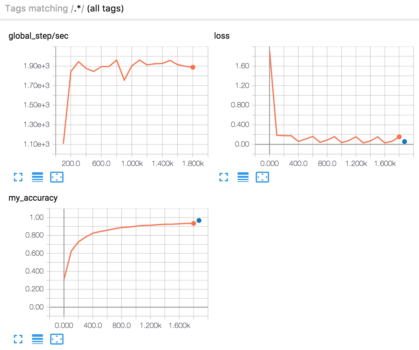
Figure 6. TensorBoard displays three graphs.

In brief, here's what the three graphs tell you:

• global_step/sec: A performance indicator, showing how many batches (gradient updates) we processed per second (y-axis) at a particular batch (x-axis). In order to see this report, you need to provide a global_step (as we did with tf.train.get_global_step()). You also need to run training for a sufficiently long time, which we do by asking the Estimator train for 500 epochs when we call its train method:
  • loss: The loss reported. The actual loss value (y-axis) doesn't mean much. The shape of the graph is what's important.

• my_accuracy: The accuracy recorded when we invoked both of the following:
• eval_metric_ops={'my_accuracy': accuracy}), during EVAL (when returning our EstimatorSpec)
• tf.summary.scalar('my_accuracy', accuracy[1]), during TRAIN

Note the following in the my_accuracy and loss graphs:

• The orange line represents TRAIN.
• The blue dot represents EVAL.

During TRAIN, orange values are recorded continuously as batches are processed, which is why it becomes a graph spanning x-axis range. By contrast, EVAL produces only a single value from processing all the evaluation steps.

As suggested in Figure 7, you may see and also selectively disable/enable the reporting for training and evaluation the left side. (Figure 7 shows that we kept reporting on for both:)

Figure 7. Enable or disable reporting.

In order to see the orange graph, you must specify a global step. This, in combination with getting global_steps/sec reported, makes it a best practice to always register a global step by passing tf.train.get_global_step()as an argument to the optimizer.minimize call.

Summary

Although pre-made Estimators can be an effective way to quickly create new models, you will often need the additional flexibility that custom Estimators provide. Fortunately, pre-made and custom Estimators follow the same programming model. The only practical difference is that you must write a model function for custom Estimators. Everything else is the same!

For more details, be sure to check out:

• The complete source code for this blog post.
• The official TensorFlow implementation of MNIST, which uses a custom estimator. This model is also an example where we take in raw pixels as numeric values without using feature columns (and input_layer).
• The TensorFlow official models repository, which may contain more curated examples using custom estimators.
• The TensorBoard video from the TensorFlow Dev Summit, which is a fun and educational introduction to TensorBoard.

Until next time - Happy TensorFlow coding!

Welcome to Part 2 of a blog series that introduces TensorFlow Datasets and Estimators. We're devoting this article to feature columns—a data structure describing the features that an Estimator requires for training and inference. As you'll see, feature columns are very rich, enabling you to represent a diverse range of data.

In Part 1, we used the pre-made Estimator DNNClassifier to train a model to predict different types of Iris flowers from four input features. That example created only numerical feature columns (of type tf.feature_column.numeric_column). Although those feature columns were sufficient to model the lengths of petals and sepals, real world data sets contain all kinds of non-numerical features. For example:

Figure 1. Non-numerical features.

How can we represent non-numerical feature types? That's exactly what this blogpost is all about.

Input to a Deep Neural Network

Let's start by asking what kind of data can we actually feed into a deep neural network? The answer is, of course, numbers (for example, tf.float32). After all, every neuron in a neural network performs multiplication and addition operations on weights and input data. Real-life input data, however, often contains non-numerical (categorical) data. For example, consider a product_class feature that can contain the following three non-numerical values:

• kitchenware
• electronics
• sports

ML models generally represent categorical values as simple vectors in which a 1 represents the presence of a value and a 0 represents the absence of a value. For example, when product_class is set to sports, an ML model would usually represent product_class as [0, 0, 1], meaning:

• 0: kitchenware is absent
• 0: electronics is absent
• 1: sports: is present

So, although raw data can be numerical or categorical, an ML model represents all features as either a number or a vector of numbers.

Introducing Feature Columns

As Figure 2 suggests, you specify the input to a model through the feature_columns argument of an Estimator (DNNClassifier for Iris). Feature Columns bridge input data (as returned by input_fn) with your model.

Figure 2. Feature columns bridge raw data with the data your model needs.

To represent features as a feature column, call functions of the tf.feature_columnpackage. This blogpost explains nine of the functions in this package. As Figure 3 shows, all nine functions return either a Categorical-Column or a Dense-Column object, except bucketized_column which inherits from both classes:

Figure 3. Feature column methods fall into two main categories and one hybrid category.

Let's look at these functions in more detail.

Numeric Column

The Iris classifier called tf.numeric_column()for all input features: SepalLength, SepalWidth, PetalLength, PetalWidth. Although tf.numeric_column() provides optional arguments, calling the function without any arguments is a perfectly easy way to specify a numerical value with the default data type (tf.float32) as input to your model. For example:

# Defaults to a tf.float32 scalar.
numeric_feature_column = tf.feature_column.numeric_column(key="SepalLength")

Use the dtype argument to specify a non-default numerical data type. For example:

# Represent a tf.float64 scalar.
numeric_feature_column = tf.feature_column.numeric_column(key="SepalLength",
                                                          dtype=tf.float64)

By default, a numeric column creates a single value (scalar). Use the shape argument to specify another shape. For example:

# Represent a 10-element vector in which each cell contains a tf.float32.
vector_feature_column = tf.feature_column.numeric_column(key="Bowling",
                                                         shape=10)

# Represent a 10x5 matrix in which each cell contains a tf.float32.
matrix_feature_column = tf.feature_column.numeric_column(key="MyMatrix",
                                                         shape=[10,5]) 

Bucketized Column

Often, you don't want to feed a number directly into the model, but instead split its value into different categories based on numerical ranges. To do so, create a bucketized column. For example, consider raw data that represents the year a house was built. Instead of representing that year as a scalar numeric column, we could split year into the following four buckets:

Figure 4. Dividing year data into four buckets.

The model will represent the buckets as follows:

Why would you want to split a number—a perfectly valid input to our model—into a categorical value like this? Well, notice that the categorization splits a single input number into a four-element vector. Therefore, the model now can learn four individual weights rather than just one. Four weights creates a richer model than one. More importantly, bucketizing enables the model to clearly distinguish between different year categories since only one of the elements is set (1) and the other three elements are cleared (0). When we just use a single number (a year) as input, the model can't distinguish categories. So, bucketing provides the model with additional important information that it can use to learn.

The following code demonstrates how to create a bucketized feature:

# A numeric column for the raw input.
numeric_feature_column = tf.feature_column.numeric_column("Year")

# Bucketize the numeric column on the years 1960, 1980, and 2000
bucketized_feature_column = tf.feature_column.bucketized_column(
    source_column = numeric_feature_column,
    boundaries = [1960, 1980, 2000])

Note the following:

• Before creating the bucketized column, we first created a numeric column to represent the raw year.
• We passed the numeric column as the first argument to tf.feature_column.bucketized_column().
• Specifying a three-element boundaries vector creates a four-element bucketized vector.

Categorical identity column

Categorical identity columns are a special case of bucketized columns. In traditional bucketized columns, each bucket represents a range of values (for example, from 1960 to 1979). In a categorical identity column, each bucket represents a single, unique integer. For example, let's say you want to represent the integer range [0, 4). (That is, you want to represent the integers 0, 1, 2, or 3.) In this case, the categorical identity mapping looks like this:

Figure 5. A categorical identity column mapping. Note that this is a one-hot encoding, not a binary numerical encoding.

So, why would you want to represent values as categorical identity columns? As with bucketized columns, a model can learn a separate weight for each class in a categorical identity column. For example, instead of using a string to represent the product_class, let's represent each class with a unique integer value. That is:

• 0="kitchenware"
• 1="electronics"
• 2="sport"

Call tf.feature_column.categorical_column_with_identity()to implement a categorical identity column. For example:

# Create a categorical output for input "feature_name_from_input_fn",
# which must be of integer type. Value is expected to be >= 0 and < num_buckets
identity_feature_column = tf.feature_column.categorical_column_with_identity(
    key='feature_name_from_input_fn', 
    num_buckets=4) # Values [0, 4)

# The 'feature_name_from_input_fn' above needs to match an integer key that is 
# returned from input_fn (see below). So for this case, 'Integer_1' or
# 'Integer_2' would be valid strings instead of 'feature_name_from_input_fn'.
# For more information, please check out Part 1 of this blog series.
def input_fn():
    ...<code>...
    return ({ 'Integer_1':[values], ..<etc>.., 'Integer_2':[values] },
            [Label_values])

Categorical vocabulary column

We cannot input strings directly to a model. Instead, we must first map strings to numeric or categorical values. Categorical vocabulary columns provide a good way to represent strings as a one-hot vector. For example:

Figure 6. Mapping string values to vocabulary columns.

As you can see, categorical vocabulary columns are kind of an enum version of categorical identity columns. TensorFlow provides two different functions to create categorical vocabulary columns:

• tf.feature_column.categorical_column_with_vocabulary_list()
• tf.feature_column.categorical_column_with_vocabulary_file()

The tf.feature_column.categorical_column_with_vocabulary_list() function maps each string to an integer based on an explicit vocabulary list. For example:

# Given input "feature_name_from_input_fn" which is a string,
# create a categorical feature to our model by mapping the input to one of 
# the elements in the vocabulary list.
vocabulary_feature_column =
    tf.feature_column.categorical_column_with_vocabulary_list(
        key="feature_name_from_input_fn",
        vocabulary_list=["kitchenware", "electronics", "sports"]) 

The preceding function has a significant drawback; namely, there's way too much typing when the vocabulary list is long. For these cases, call tf.feature_column.categorical_column_with_vocabulary_file()instead, which lets you place the vocabulary words in a separate file. For example:

# Given input "feature_name_from_input_fn" which is a string,
# create a categorical feature to our model by mapping the input to one of 
# the elements in the vocabulary file
vocabulary_feature_column =
    tf.feature_column.categorical_column_with_vocabulary_file(
        key="feature_name_from_input_fn",
        vocabulary_file="product_class.txt",
        vocabulary_size=3)

# product_class.txt should have one line for vocabulary element, in our case:
kitchenware
electronics
sports

Using hash buckets to limit categories

So far, we've worked with a naively small number of categories. For example, our product_class example has only 3 categories. Often though, the number of categories can be so big that it's not possible to have individual categories for each vocabulary word or integer because that would consume too much memory. For these cases, we can instead turn the question around and ask, "How many categories am I willing to have for my input?" In fact, the tf.feature_column.categorical_column_with_hash_buckets()function enables you to specify the number of categories. For example, the following code shows how this function calculates a hash value of the input, then puts it into one of the hash_bucket_size categories using the modulo operator:

# Create categorical output for input "feature_name_from_input_fn".
# Category becomes: hash_value("feature_name_from_input_fn") % hash_bucket_size
hashed_feature_column =
    tf.feature_column.categorical_column_with_hash_bucket(
        key = "feature_name_from_input_fn",
        hash_buckets_size = 100) # The number of categories

At this point, you might rightfully think: "This is crazy!" After all, we are forcing the different input values to a smaller set of categories. This means that two, probably completely unrelated inputs, will be mapped to the same category, and consequently mean the same thing to the neural network. Figure 7 illustrates this dilemma, showing that kitchenware and sports both get assigned to category (hash bucket) 12:

Figure 7. Representing data in hash buckets.

As with many counterintuitive phenomena in machine learning, it turns out that hashing often works well in practice. That's because hash categories provide the model with some separation. The model can use additional features to further separate kitchenware from sports.

Feature crosses

The last categorical column we'll cover allows us to combine multiple input features into a single one. Combining features, better known as feature crosses, enables the model to learn separate weights specifically for whatever that feature combination means.

More concretely, suppose we want our model to calculate real estate prices in Atlanta, GA. Real-estate prices within this city vary greatly depending on location. Representing latitude and longitude as separate features isn't very useful in identifying real-estate location dependencies; however, crossing latitude and longitude into a single feature can pinpoint locations. Suppose we represent Atlanta as a grid of 100x100 rectangular sections, identifying each of the 10,000 sections by a cross of its latitude and longitude. This cross enables the model to pick up on pricing conditions related to each individual section, which is a much stronger signal than latitude and longitude alone.

Figure 8 shows our plan, with the latitude & longitude values for the corners of the city:

Figure 8. Map of Atlanta. Imagine this map divided into 10,000 sections of equal size.

For the solution, we used a combination of some feature columns we've looked at before, as well as the tf.feature_columns.crossed_column()function.

# In our input_fn, we convert input longitude and latitude to integer values
# in the range [0, 100)
def input_fn():
    # Using Datasets, read the input values for longitude and latitude
    latitude = ...   # A tf.float32 value
    longitude = ...  # A tf.float32 value

    # In our example we just return our lat_int, long_int features.
    # The dictionary of a complete program would probably have more keys.
    return { "latitude": latitude, "longitude": longitude, ...}, labels

# As can be see from the map, we want to split the latitude range
# [33.641336, 33.887157] into 100 buckets. To do this we use np.linspace
# to get a list of 99 numbers between min and max of this range.
# Using this list we can bucketize latitude into 100 buckets.
latitude_buckets = list(np.linspace(33.641336, 33.887157, 99))
latitude_fc = tf.feature_column.bucketized_column(
    tf.feature_column.numeric_column('latitude'),
    latitude_buckets)

# Do the same bucketization for longitude as done for latitude.
longitude_buckets = list(np.linspace(-84.558798, -84.287259, 99))
longitude_fc = tf.feature_column.bucketized_column(
    tf.feature_column.numeric_column('longitude'), longitude_buckets)

# Create a feature cross of fc_longitude x fc_latitude.
fc_san_francisco_boxed = tf.feature_column.crossed_column(
    keys=[latitude_fc, longitude_fc],
    hash_bucket_size=1000) # No precise rule, maybe 1000 buckets will be good?

You may create a feature cross from either of the following:

• Feature names; that is, names from the dict returned from input_fn.
• Any Categorical Column (see Figure 3), except categorical_column_with_hash_bucket.

When feature columns latitude_fc and longitude_fc are crossed, TensorFlow will create 10,000 combinations of (latitude_fc, longitude_fc) organized as follows:

(0,0),(0,1)...  (0,99)
(1,0),(1,1)...  (1,99)
…, …,          ...
(99,0),(99,1)...(99, 99)

The function tf.feature_column.crossed_column performs a hash calculation on these combinations and then slots the result into a category by performing a modulo operation with hash_bucket_size. As discussed before, performing the hash and modulo function will probably result in category collisions; that is, multiple (latitude, longitude) feature crosses will end up in the same hash bucket. In practice though, performing feature crosses still provides significant value to the learning capability of your models.

Somewhat counterintuitively, when creating feature crosses, you typically still should include the original (uncrossed) features in your model. For example, provide not only the (latitude, longitude) feature cross but also latitude and longitude as separate features. The separate latitude and longitude features help the model separate the contents of hash buckets containing different feature crosses.

See this link for a full code example for this. Also, the reference section at the end of this post for lots more examples of feature crossing.

Indicator and embedding columns

Indicator columns and embedding columns never work on features directly, but instead take categorical columns as input.

When using an indicator column, we're telling TensorFlow to do exactly what we've seen in our categorical product_class example. That is, an indicator column treats each category as an element in a one-hot vector, where the matching category has value 1 and the rest have 0s:

Figure 9. Representing data in indicator columns.

Here's how you create an indicator column:

categorical_column = ... # Create any type of categorical column, see Figure 3

# Represent the categorical column as an indicator column.
# This means creating a one-hot vector with one element for each category.
indicator_column = tf.feature_column.indicator_column(categorical_column)

Now, suppose instead of having just three possible classes, we have a million. Or maybe a billion. For a number of reasons (too technical to cover here), as the number of categories grow large, it becomes infeasible to train a neural network using indicator columns.

We can use an embedding column to overcome this limitation. Instead of representing the data as a one-hot vector of many dimensions, anembedding column represents that data as a lower-dimensional, ordinary vector in which each cell can contain any number, not just 0 or 1. By permitting a richer palette of numbers for every cell, an embedding column contains far fewer cells than an indicator column.

Let's look at an example comparing indicator and embedding columns. Suppose our input examples consists of different words from a limited palette of only 81 words. Further suppose that the data set provides provides the following input words in 4 separate examples:

• "dog"
• "spoon"
• "scissors"
• "guitar"

In that case, Figure 10 illustrates the processing path for embedding columns or Indicator columns.

Figure 10. An embedding column stores categorical data in a lower-dimensional vector than an indicator column. (We just placed random numbers into the embedding vectors; training determines the actual numbers.)

When an example is processed, one of the categorical_column_with...functions maps the example string to a numerical categorical value. For example, a function maps "spoon" to [32]. (The 32comes from our imagination—the actual values depend on the mapping function.) You may then represent these numerical categorical values in either of the following two ways:

• As an indicator column. A function converts each numeric categorical value into an 81-element vector (because our palette consists of 81 words), placing a 1 in the index of the categorical value (0, 32, 79, 80) and a 0 in all the other positions.
• As an embedding column. A function uses the numerical categorical values (0, 32, 79, 80) as indices to a lookup table. Each slot in that lookup table contains a 3-element vector.

How do the values in the embeddings vectors magically get assigned? Actually, the assignments happen during training. That is, the model learns the best way to map your input numeric categorical values to the embeddings vector value in order to solve your problem. Embedding columns increase your model's capabilities, since an embeddings vector learns new relationships between categories from the training data.

Why is the embedding vector size 3 in our example? Well, the following "formula" provides a general rule of thumb about the number of embedding dimensions:

embedding_dimensions =  number_of_categories**0.25

That is, the embedding vector dimension should be the 4th root of the number of categories. Since our vocabulary size in this example is 81, the recommended number of dimensions is 3:

3 =  81**0.25

Note that this is just a general guideline; you can set the number of embedding dimensions as you please.

Call tf.feature_column.embedding_columnto create an embedding_column. The dimension of the embedding vector depends on the problem at hand as described above, but common values go as low as 3 all the way to 300 or even beyond:

categorical_column = ... # Create any categorical column shown in Figure 3.

# Represent the categorical column as an embedding column.
# This means creating a one-hot vector with one element for each category.
embedding_column = tf.feature_column.embedding_column(
    categorical_column=categorical_column,
    dimension=dimension_of_embedding_vector)

Embeddings is a big topic within machine learning. This information was just to get you started using them as feature columns. Please see the end of this post for more information.

Passing feature columns to Estimators

Still there? I hope so, because we only have a tiny bit left before you've graduated from the basics of feature columns.

As we saw in Figure 1, feature columns map your input data (described by the feature dictionary returned from input_fn) to values fed to your model. You specify feature columns as a list to a feature_columns argument of an estimator. Note that the feature_columns argument(s) vary depending on the Estimator:

• LinearClassifierand LinearRegressor:
  • Accept all types of feature column.
  • DNNClassifierand DNNRegressor:
    • Only accept dense columns, see Figure 3. Other column types must be wrapped in either an indicator_column or embedding_column as described earlier.
    • DNNLinearCombinedClassifierand DNNLinearCombinedRegressor:
      • The linear_feature_columns argument can accept any column type, like the LinearClassifier and LinearRegressor above.
      • The dnn_feature_columns argument however is limited to dense columns, like DNNClassifier and DNNRegressorabove.

The reason for the above rules are beyond the scope of this introductory post, but we will make sure to cover it in a future blogpost.

Summary

Use feature columns to map your input data to the representations you feed your model. We only used numeric_column in Part 1 of this series , but working with the other functions described in this post, you can easily create other feature columns.

For more details on feature columns, be sure to check out:

• Josh Gordon's video on Feature Engineering
• And from the same author, a Jupyter notebook
• The TensorFlow - Wide & Deep Tutorial
• Examplesof DNNs and linear models that use feature columns

If you want to learn more about embeddings:

• Deep Learning, NLP, and representations (Colah's blog)
• And checkout the TensorFlow Embedding Projector

TensorFlow 1.3 introduces two important features that you should try out:

• Datasets: A completely new way of creating input pipelines (that is, reading data into your program).

• Estimators: A high-level way to create TensorFlow models. Estimators include pre-made models for common machine learning tasks, but you can also use them to create your own custom models.

Below you can see how they fit in the TensorFlow architecture. Combined, they offer an easy way to create TensorFlow models and to feed data to them:

Our Example Model

To explore these features we're going to build a model and show you relevant code snippets. The complete code is available here, including instructions for getting the training and test files. Note that the code was written to demonstrate how Datasets and Estimators work functionally, and was not optimized for maximum performance.

The trained model categorizes Iris flowers based on four botanical features (sepal length, sepal width, petal length, and petal width). So, during inference, you can provide values for those four features and the model will predict that the flower is one of the following three beautiful variants:

We're going to train a Deep Neural Network Classifier with the below structure. All input and output values will be float32, and the sum of the output values will be 1 (as we are predicting the probability for each individual Iris type):

For example, an output result might be 0.05 for Iris Setosa, 0.9 for Iris Versicolor, and 0.05 for Iris Virginica, which indicates a 90% probability that this is an Iris Versicolor.

Alright! Now that we have defined the model, let's look at how we can use Datasets and Estimators to train it and make predictions.

Introducing The Datasets

Datasets is a new way to create input pipelines to TensorFlow models. This API is much more performant than using feed_dict or the queue-based pipelines, and it's cleaner and easier to use. Although Datasets still resides in tf.contrib.data at 1.3, we expect to move this API to core at 1.4, so it's high time to take it for a test drive.

At a high-level, the Datasets consists of the following classes:

Where:

• Dataset: Base class containing methods to create and transform datasets. Also allows you initialize a dataset from data in memory, or from a Python generator.
• TextLineDataset: Reads lines from text files.
• TFRecordDataset: Reads records from TFRecord files.
• FixedLengthRecordDataset: Reads fixed size records from binary files.
• Iterator: Provides a way to access one dataset element at a time.

Our dataset

To get started, let's first look at the dataset we will use to feed our model. We'll read data from a CSV file, where each row will contain five values-the four input values, plus the label:

The label will be:

• 0 for Iris Setosa
• 1 for Versicolor
• 2 for Virginica.

Representing our dataset

To describe our dataset, we first create a list of our features:

feature_names = [
    'SepalLength',
    'SepalWidth',
    'PetalLength',
    'PetalWidth']

When we train our model, we'll need a function that reads the input file and returns the feature and label data. Estimators requires that you create a function of the following format:

def input_fn():
    ...<code>...
    return ({ 'SepalLength':[values], ..<etc>.., 'PetalWidth':[values] },
            [IrisFlowerType])

The return value must be a two-element tuple organized as follows: :

• The first element must be a dict in which each input feature is a key, and then a list of values for the training batch.
• The second element is a list of labels for the training batch.

Since we are returning a batch of input features and training labels, it means that all lists in the return statement will have equal lengths. Technically speaking, whenever we referred to "list" here, we actually mean a 1-d TensorFlow tensor.

To allow simple reuse of the input_fn we're going to add some arguments to it. This allows us to build input functions with different settings. The arguments are pretty straightforward:

• file_path: The data file to read.
• perform_shuffle: Whether the record order should be randomized.
• repeat_count: The number of times to iterate over the records in the dataset. For example, if we specify 1, then each record is read once. If we specify None, iteration will continue forever.

Here's how we can implement this function using the Dataset API. We will wrap this in an "input function" that is suitable when feeding our Estimator model later on:

def my_input_fn(file_path, perform_shuffle=False, repeat_count=1):
   def decode_csv(line):
       parsed_line = tf.decode_csv(line, [[0.], [0.], [0.], [0.], [0]])
       label = parsed_line[-1:] # Last element is the label
       del parsed_line[-1] # Delete last element
       features = parsed_line # Everything (but last element) are the features
       d = dict(zip(feature_names, features)), label
       return d

   dataset = (tf.contrib.data.TextLineDataset(file_path) # Read text file
       .skip(1) # Skip header row
       .map(decode_csv)) # Transform each elem by applying decode_csv fn
   if perform_shuffle:
       # Randomizes input using a window of 256 elements (read into memory)
       dataset = dataset.shuffle(buffer_size=256)
   dataset = dataset.repeat(repeat_count) # Repeats dataset this # times
   dataset = dataset.batch(32)  # Batch size to use
   iterator = dataset.make_one_shot_iterator()
   batch_features, batch_labels = iterator.get_next()
   return batch_features, batch_labels

Note the following: :

• TextLineDataset: The Dataset API will do a lot of memory management for you when you're using its file-based datasets. You can, for example, read in dataset files much larger than memory or read in multiple files by specifying a list as argument.
• shuffle: Reads buffer_size records, then shuffles (randomizes) their order.
• map: Calls the decode_csv function with each element in the dataset as an argument (since we are using TextLineDataset, each element will be a line of CSV text). Then we apply decode_csv to each of the lines.
• decode_csv: Splits each line into fields, providing the default values if necessary. Then returns a dict with the field keys and field values. The map function updates each elem (line) in the dataset with the dict.

That's an introduction to Datasets! Just for fun, we can now use this function to print the first batch:

next_batch = my_input_fn(FILE, True) # Will return 32 random elements

# Now let's try it out, retrieving and printing one batch of data.
# Although this code looks strange, you don't need to understand
# the details.
with tf.Session() as sess:
    first_batch = sess.run(next_batch)
print(first_batch)

# Output
({'SepalLength': array([ 5.4000001, ...<repeat to 32 elems>], dtype=float32),
  'PetalWidth': array([ 0.40000001, ...<repeat to 32 elems>], dtype=float32),
  ...
 },
 [array([[2], ...<repeat to 32 elems>], dtype=int32) # Labels
)

That's actually all we need from the Dataset API to implement our model. Datasets have a lot more capabilities though; please see the end of this post where we have collected more resources.

Introducing Estimators

Estimators is a high-level API that reduces much of the boilerplate code you previously needed to write when training a TensorFlow model. Estimators are also very flexible, allowing you to override the default behavior if you have specific requirements for your model.

There are two possible ways you can build your model using Estimators:

• Pre-made Estimator - These are predefined estimators, created to generate a specific type of model. In this blog post, we will use the DNNClassifier pre-made estimator.
• Estimator (base class) - Gives you complete control of how your model should be created by using a model_fn function. We will cover how to do this in a separate blog post.

Here is the class diagram for Estimators:

We hope to add more pre-made Estimators in future releases.

As you can see, all estimators make use of input_fn that provides the estimator with input data. In our case, we will reuse my_input_fn, which we defined for this purpose.

The following code instantiates the estimator that predicts the Iris flower type:

# Create the feature_columns, which specifies the input to our model.
# All our input features are numeric, so use numeric_column for each one.
feature_columns = [tf.feature_column.numeric_column(k) for k in feature_names]

# Create a deep neural network regression classifier.
# Use the DNNClassifier pre-made estimator
classifier = tf.estimator.DNNClassifier(
   feature_columns=feature_columns, # The input features to our model
   hidden_units=[10, 10], # Two layers, each with 10 neurons
   n_classes=3,
   model_dir=PATH) # Path to where checkpoints etc are stored

We now have a estimator that we can start to train.

Training the model

Training is performed using a single line of TensorFlow code:

# Train our model, use the previously function my_input_fn
# Input to training is a file with training example
# Stop training after 8 iterations of train data (epochs)
classifier.train(
   input_fn=lambda: my_input_fn(FILE_TRAIN, True, 8))

But wait a minute... what is this "lambda: my_input_fn(FILE_TRAIN, True, 8)" stuff? That is where we hook up Datasets with the Estimators! Estimators needs data to perform training, evaluation, and prediction, and it uses the input_fn to fetch the data. Estimators require an input_fn with no arguments, so we create a function with no arguments using lambda, which calls our input_fn with the desired arguments: the file_path, shuffle setting, and repeat_count. In our case, we use our my_input_fn, passing it:

• FILE_TRAIN, which is the training data file.
• True, which tells the Estimator to shuffle the data.
• 8, which tells the Estimator to and repeat the dataset 8 times.

Evaluating Our Trained Model

Ok, so now we have a trained model. How can we evaluate how well it's performing? Fortunately, every Estimator contains an evaluatemethod:

# Evaluate our model using the examples contained in FILE_TEST
# Return value will contain evaluation_metrics such as: loss & average_loss
evaluate_result = estimator.evaluate(
   input_fn=lambda: my_input_fn(FILE_TEST, False, 4)
print("Evaluation results")
for key in evaluate_result:
   print("   {}, was: {}".format(key, evaluate_result[key]))

In our case, we reach an accuracy of about ~93%. There are various ways of improving this accuracy, of course. One way is to simply run the program over and over. Since the state of the model is persisted (in model_dir=PATH above), the model will improve the more iterations you train it, until it settles. Another way would be to adjust the number of hidden layers or the number of nodes in each hidden layer. Feel free to experiment with this; please note, however, that when you make a change, you need to remove the directory specified in model_dir=PATH, since you are changing the structure of the DNNClassifier.

Making Predictions Using Our Trained Model

And that's it! We now have a trained model, and if we are happy with the evaluation results, we can use it to predict an Iris flower based on some input. As with training, and evaluation, we make predictions using a single function call:

# Predict the type of some Iris flowers.
# Let's predict the examples in FILE_TEST, repeat only once.
predict_results = classifier.predict(
    input_fn=lambda: my_input_fn(FILE_TEST, False, 1))
print("Predictions on test file")
for prediction in predict_results:
   # Will print the predicted class, i.e: 0, 1, or 2 if the prediction
   # is Iris Sentosa, Vericolor, Virginica, respectively.
   print prediction["class_ids"][0] 

Making Predictions on Data in Memory

The preceding code specified FILE_TEST to make predictions on data stored in a file, but how could we make predictions on data residing in other sources, for example, in memory? As you may guess, this does not actually require a change to our predict call. Instead, we configure the Dataset API to use a memory structure as follows:

# Let create a memory dataset for prediction.
# We've taken the first 3 examples in FILE_TEST.
prediction_input = [[5.9, 3.0, 4.2, 1.5],  # -> 1, Iris Versicolor
                    [6.9, 3.1, 5.4, 2.1],  # -> 2, Iris Virginica
                    [5.1, 3.3, 1.7, 0.5]]  # -> 0, Iris Sentosa
def new_input_fn():
   def decode(x):
       x = tf.split(x, 4) # Need to split into our 4 features
       # When predicting, we don't need (or have) any labels
       return dict(zip(feature_names, x)) # Then build a dict from them

   # The from_tensor_slices function will use a memory structure as input
   dataset = tf.contrib.data.Dataset.from_tensor_slices(prediction_input)
   dataset = dataset.map(decode)
   iterator = dataset.make_one_shot_iterator()
   next_feature_batch = iterator.get_next()
   return next_feature_batch, None # In prediction, we have no labels

# Predict all our prediction_input
predict_results = classifier.predict(input_fn=new_input_fn)

# Print results
print("Predictions on memory data")
for idx, prediction in enumerate(predict_results):
   type = prediction["class_ids"][0] # Get the predicted class (index)
   if type == 0:
       print("I think: {}, is Iris Sentosa".format(prediction_input[idx]))
   elif type == 1:
       print("I think: {}, is Iris Versicolor".format(prediction_input[idx]))
   else:
       print("I think: {}, is Iris Virginica".format(prediction_input[idx])

Dataset.from_tensor_slides() is designed for small datasets that fit in memory. When using TextLineDataset as we did for training and evaluation, you can have arbitrarily large files, as long as your memory can manage the shuffle buffer and batch sizes.

Freebies

Using a pre-made Estimator like DNNClassifier provides a lot of value. In addition to being easy to use, pre-made Estimators also provide built-in evaluation metrics, and create summaries you can see in TensorBoard. To see this reporting, start TensorBoard from your command-line as follows:

# Replace PATH with the actual path passed as model_dir argument when the
# DNNRegressor estimator was created.
tensorboard --logdir=PATH 

The following diagrams show some of the data that TensorBoard will provide:

Summary

In this this blogpost, we explored Datasets and Estimators. These are important APIs for defining input data streams and creating models, so investing time to learn them is definitely worthwhile!

For more details, be sure to check out

• The complete source code used in this blogpost is available here.
• Josh Gordon's excellent Jupyter notebook on the matter. Using that notebook, you will learn how to run a more extensive example that has many different types of features (inputs). As you recall from our model, we just used numeric features.
• For Datasets, see a new chapter in the Programmer's guide and reference documentation.
• For Estimators, see a new chapter in the Programmer's guide and reference documentation.

But it doesn't stop here. We will shortly publish more posts that describe how these APIs work, so stay tuned for that!

Until then, Happy TensorFlow coding!