Tag Archives: datasets

Introducing the Schema-Guided Dialogue Dataset for Conversational Assistants


Today's virtual assistants help users to accomplish a wide variety of tasks, including finding flights, searching for nearby events and movies, making reservations, sourcing information from the web and more. They provide this functionality by offering a unified natural language interface to a wide variety of services across the web. Large-scale virtual assistants, like Google Assistant, need to integrate with a large and constantly increasing number of services, each with potentially overlapping functionality, over a wide variety of domains. Supporting new services with ease, without collection of additional data or retraining the model, and reducing maintenance workload are necessary to accommodate future growth. Despite tremendous progress, however, these challenges have often been overlooked in state-of-the-art models. This is due, in part, to the absence of suitable datasets that match the scale and complexity confronted by such virtual assistants.

In our recent paper, “Towards Scalable Multi-domain Conversational Agents: The Schema-Guided Dialogue Dataset”, we introduce a new dataset to address these problems. The Schema-Guided Dialogue dataset (SGD) is the largest publicly available corpus of task-oriented dialogues, with over 18,000 dialogues spanning 17 domains. Equipped with various annotations, this dataset is designed to serve as an effective testbed for intent prediction, slot filling, state tracking (i.e., estimating the user's goal) and language generation, among other tasks for large-scale virtual assistants. We also propose a schema-guided approach for building virtual assistants as a solution to the aforementioned challenges. Our approach utilizes a single model across all services and domains, with no domain-specific parameters. Based on the schema-guided approach and building on the power of pre-trained language models like BERT, we open source a model for dialogue state tracking, which is applicable in a zero-shot setting (i.e., with no training data for new services and APIs) while remaining competitive in the regular setting.

The Dataset
The primary goal of releasing the SGD dataset is to confront many real-world challenges that are not sufficiently captured by existing datasets. The SGD dataset consists of over 18k annotated multi-domain, task-oriented conversations between a human and a virtual assistant. These conversations involve interactions with services and APIs spanning 17 domains, ranging from banks and events to media, calendar, travel, and weather. For most of these domains, the SGD dataset contains multiple different APIs, many of which have overlapping functionalities but different interfaces, which reflects common real-world scenarios. SGD is the first dataset to cover such a wide variety of domains and provide multiple APIs per domain. Furthermore, to quantify the robustness of models to changes in API interfaces or to the addition of new APIs, the evaluation set contains many new services that are not present in the training set.

For the creation of the SGD dataset, we have prioritized the variety and accuracy of annotations in the included dialogues. To begin with, dialogues were collected by interaction between two people using a Wizard-of-Oz style process, followed by crowdsourced annotation. Initial efforts revealed the difficulty in obtaining consistent annotations using this method, so we developed a new data collection process that minimized the need for complex manual annotation, and considerably reduced the time and cost of data collection.

For this alternate approach, we developed a multi-domain dialogue simulator that generates dialogue skeletons over an arbitrary combination of APIs, along with the corresponding annotations, such as dialogue state and system actions. The simulator consists of two agents playing the role of the user and the assistant. Both the agents interact with each other using a finite set of actions denoting dialogue semantics with transitions specified through a probabilistic automaton, designed to capture a wide variety of dialogue trajectories. The actions generated by the simulator are converted into natural language utterances using a set of templates. Crowdsourcing is used only for paraphrasing these templatized utterances in order to make the dialogue more natural and coherent. This setup eliminates the need for complicated domain-specific instructions while keeping the crowdsourcing task simple and yields natural dialogues with consistent, high quality annotations.
Steps for obtaining dialogues, with assistant turns marked in red and user turns in blue. Left: The simulator generates a dialogue skeleton using a finite set of actions. Center: Actions are converted into utterances using templates (~50 per service) and slot values are replaced with natural variations. Right: Paraphrasing via crowdsourcing to make the flow cohesive.
The Schema-Guided Approach
With the availability of the SGD dataset, it is now possible to train virtual assistants to support the diversity of services available on the web. A common approach to do this requires a large master schema that lists all supported functions and their parameters. However, it is difficult to develop a master schema catering to all possible use cases. Even if that problem is solved, a master schema would complicate integration of new or small-scale services and would increase the maintenance workload of the assistant. Furthermore, while there are many similar concepts across services that can be jointly modeled, for example, the similarities in logic for querying or specifying the number of movie tickets, flight tickets or concert tickets, the master schema approach does not facilitate joint modeling of such concepts, unless an explicit mapping between them is manually defined.

The new schema-guided approach we propose addresses these limitations. This approach does not require the definition of a master schema for the assistant. Instead, each service or API provides a natural language description of the functions listed in its schema along with their associated attributes. These descriptions are then used to learn a distributed semantic representation of the schema, which is given as an additional input to the dialogue system. The dialogue system is then implemented as a single unified model, containing no domain or service specific parameters. This unified model facilitates representation of common knowledge between similar concepts in different services, while the use of distributed representations of the schema makes it possible to operate over new services that are not present in the training data. We have implemented this approach in our open-sourced dialogue state tracking model.

Eighth Dialogue System Technology Challenge
The Dialog System Technology Challenges (DSTCs) are a series of research competitions to accelerate the development of new dialogue technologies. This year, Google organized one of the tracks, "Schema-Guided Dialogue State Tracking", as part of the recently concluded 8th DSTC. We received submissions from a total of 25 teams from both industry and academia, which will be presented at the DSTC8 workshop at AAAI-20.

We believe that this dataset will act as a good benchmark for building large-scale dialogue models. We are excited and looking forward to all the innovative ways in which the research community will use it for the advancement of dialogue technologies.

Acknowledgements
This post reflects the work of our co-authors Xiaoxue Zang, Srinivas Sunkara and Raghav Gupta. We also thank Amir Fayazi and Maria Wang for help with data collection and Guan-Lin Chao for insights on model design and implementation.

Source: Google AI Blog


Releasing PAWS and PAWS-X: Two New Datasets to Improve Natural Language Understanding Models


Word order and syntactic structure have a large impact on sentence meaning — even small perturbations in word order can completely change interpretation. For example, consider the following related sentences:
  1. Flights from New York to Florida.
  2. Flights to Florida from New York.
  3. Flights from Florida to New York.
All three have the same set of words. However, 1 and 2 have the same meaning — known as paraphrase pairs — while 1 and 3 have very different meanings — known as non-paraphrase pairs. The task of identifying whether pairs are paraphrase or not is called paraphrase identification, and this task is important to many real-world natural language understanding (NLU) applications such as question answering. Perhaps surprisingly, even state-of-the-art models, like BERT, would fail to correctly identify the difference between many non-paraphrase pairs like 1 and 3 above if trained only on existing NLU datasets. This is because existing datasets lack training pairs like this, so it is hard for machine learning models to learn this pattern even if they have the capability to understand complex contextual phrasings.

To address this, we are releasing two new datasets for use in the research community: Paraphrase Adversaries from Word Scrambling (PAWS) in English, and PAWS-X, an extension of the PAWS dataset to six typologically distinct languages: French, Spanish, German, Chinese, Japanese, and Korean. Both datasets contain well-formed sentence pairs with high lexical overlap, in which about half of the pairs are paraphrase and others are not. Including new pairs in training data for state-of-the-art models improves their accuracy on this problem from <50% to 85-90%. In contrast, models that do not capture non-local contextual information fail even with new training examples. The new datasets therefore provide an effective instrument for measuring the sensitivity of models to word order and structure.

The PAWS dataset contains 108,463 human-labeled pairs in English, sourced from Quora Question Pairs (QQP) and Wikipedia pages. PAWS-X contains 23,659 human translated PAWS evaluation pairs and 296,406 machine translated training pairs. The table below gives detailed statistics of the datasets.
PAWS PAWS-X
Language English English Chinese French German Japanese Korean Spanish
(QQP) (Wiki) (Wiki) (Wiki) (Wiki) (Wiki) (Wiki) (Wiki)
Training 11,988 79,798 49,401 49,401 49,401 49,401 49,401 49,401
Dev 677 8,000 1,984 1,992 1,932 1,980 1,965 1,962
Test - 8,000 1,975 1,985 1,967 1,946 1,972 1,999
† The training set of PAWS-X is machine translated from a subset of the PAWS Wiki dataset in English.
Creating the PAWS Dataset in English
In “PAWS: Paraphrase Adversaries from Word Scrambling,” we introduce a workflow for generating pairs of sentences that have high word overlap, but which are balanced with respect to whether they are paraphrases or not. To generate examples, source sentences are first passed to a specialized language model that creates word-swapped variants that are still semantically meaningful, but ambiguous as to whether they are paraphrase pairs or not. These were then judged by human raters for grammaticality and then multiple raters judged whether they were paraphrases of each other. 
PAWS corpus creation workflow.
One problem with this swapping strategy is that it tends to produce pairs that aren't paraphrases (e.g., "why do bad things happen to good people" != "why do good things happen to bad people"). In order to ensure balance between paraphrases and non-paraphrases, we added other examples based on back-translation. Back-translation has the opposite bias as it tends to preserve meaning while changing word order and word choice. These two strategies lead to PAWS being balanced overall, especially for the Wikipedia portion.

Creating the Multilingual PAWS-X Dataset
After creating PAWS, we extended it to six more languages: Chinese, French, German, Korean, Japanese, and Spanish. We hired human translators to translate the development and test sets, and used a neural machine translation (NMT) service to translate the training set.
We obtained human translations (native speakers) on a random sample of 4,000 sentence pairs from the PAWS development set for each of the six languages (48,000 translations). Each sentence in a pair is presented independently so that translation is not affected by context. A randomly sampled subset was validated by a second worker. The final dataset has less than 5% word level error rate.
Note, we allowed professionals to not translate a sentence if it was incomplete or ambiguous. On average, less than 2% of the pairs were not translated, and we simply excluded them. The final translated pairs are split then into new development and test sets, ~2,000 pairs for each.
Examples of human translated pairs for German(de) and Chinese(zh).
Language Understanding with PAWS and PAWS-X
We train multiple models on the created dataset and measure the classification accuracy on the eval set. When trained with PAWS, strong models, such as BERT and DIIN, show remarkable improvement over when they are trained on the existing Quora Question Pairs (QQP) dataset. For example, on the PAWS data sourced from QQP (PAWS-QQP), BERT gets only 33.5 accuracy if trained on existing QQP, but it recovers to 83.1 accuracy when given PAWS training examples. Unlike BERT, a simple Bag-of-Words (BOW) model fails to learn from PAWS training examples, demonstrating its weakness at capturing non-local contextual information. These results demonstrate that PAWS effectively measures sensitivity of models to word order and structure.
Accuracy on PAWS-QQP Eval Set (English).
The figure below shows the performance of the popular multilingual BERT model on PAWS-X using several common strategies:
  1. Zero Shot: The model is trained on the PAWS English training data, and then directly evaluated on all others. Machine translation is not involved in this strategy.
  2. Translate Test: Train a model using the English training data, and machine-translate all test examples to English for evaluation.
  3. Translate Train: The English training data is machine-translated into each target language to provide data to train each model.
  4. Merged: Train a multilingual model on all languages, including the original English pairs and machine-translated data in all other languages.
The results show that cross-lingual techniques help, while it also leaves considerable headroom to drive multilingual research on the problem of paraphrase identification
Accuracy of PAWS-X Test Set using BERT Models.
It is our hope that these datasets will be useful to the research community to drive further progress on multilingual models that better exploit structure, context, and pairwise comparisons.

Acknowledgements
The core team includes Luheng He, Jason Baldridge, Chris Tar. We would like to thank the Language team in Google Research, especially Emily Pitler, for the insightful comments that contributed to our papers. Many thanks also to Ashwin Kakarla, Henry Jicha, and Mengmeng Niu, for the help with the annotations.

Source: Google AI Blog


Contributing Data to Deepfake Detection Research


Deep learning has given rise to technologies that would have been thought impossible only a handful of years ago. Modern generative models are one example of these, capable of synthesizing hyperrealistic images, speech, music, and even video. These models have found use in a wide variety of applications, including making the world more accessible through text-to-speech, and helping generate training data for medical imaging.

Like any transformative technology, this has created new challenges. So-called "deepfakes"—produced by deep generative models that can manipulate video and audio clips—are one of these. Since their first appearance in late 2017, many open-source deepfake generation methods have emerged, leading to a growing number of synthesized media clips. While many are likely intended to be humorous, others could be harmful to individuals and society.

Google considers these issues seriously. As we published in our AI Principles last year, we are committed to developing AI best practices to mitigate the potential for harm and abuse. Last January, we announced our release of a dataset of synthetic speech in support of an international challenge to develop high-performance fake audio detectors. The dataset was downloaded by more than 150 research and industry organizations as part of the challenge, and is now freely available to the public.

Today, in collaboration with Jigsaw, we're announcing the release of a large dataset of visual deepfakes we've produced that has been incorporated into the Technical University of Munich and the University Federico II of Naples’ new FaceForensics benchmark, an effort that Google co-sponsors. The incorporation of these data into the FaceForensics video benchmark is in partnership with leading researchers, including Prof. Matthias Niessner, Prof. Luisa Verdoliva and the FaceForensics team. You can download the data on the FaceForensics github page.
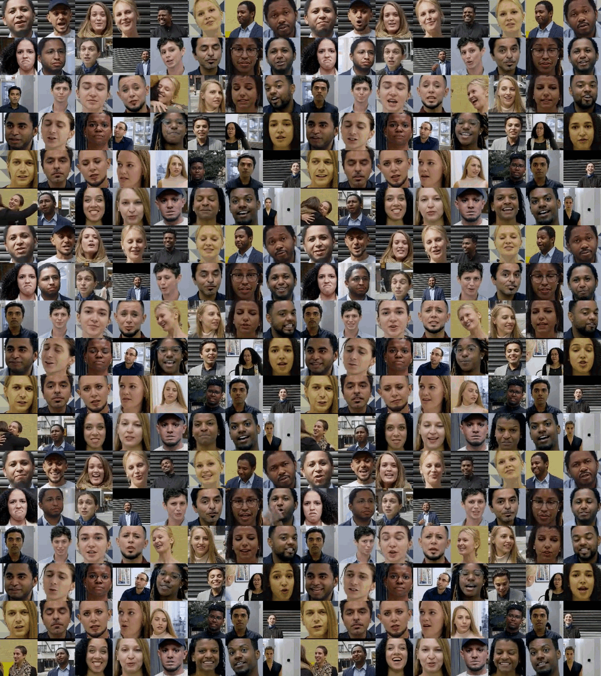
A sample of videos from Google’s contribution to the FaceForensics benchmark. To generate these, pairs of actors were selected randomly and deep neural networks swapped the face of one actor onto the head of another.
To make this dataset, over the past year we worked with paid and consenting actors to record hundreds of videos. Using publicly available deepfake generation methods, we then created thousands of deepfakes from these videos. The resulting videos, real and fake, comprise our contribution, which we created to directly support deepfake detection efforts. As part of the FaceForensics benchmark, this dataset is now available, free to the research community, for use in developing synthetic video detection methods.
Actors were filmed in a variety of scenes. Some of these actors are pictured here (top) with an example deepfake (bottom), which can be a subtle or drastic change, depending on the other actor used to create them.
Since the field is moving quickly, we'll add to this dataset as deepfake technology evolves over time, and we’ll continue to work with partners in this space. We firmly believe in supporting a thriving research community around mitigating potential harms from misuses of synthetic media, and today's release of our deepfake dataset in the FaceForensics benchmark is an important step in that direction.

Acknowledgements
Special thanks to all our team members and collaborators who work on this project with us: Daisy Stanton, Per Karlsson, Alexey Victor Vorobyov, Thomas Leung, Jeremiah "Spudde" Childs, Christoph Bregler, Andreas Roessler, Davide Cozzolino, Justus Thies, Luisa Verdoliva, Matthias Niessner, and the hard-working actors and film crew who helped make this dataset possible.

Source: Google AI Blog


Adding Diversity to Images with Open Images Extended


Recently, we introduced the Inclusive Images Kaggle competition, part of the NeurIPS 2018 Competition Track, with the goal of stimulating research into the effect of geographic skews in training datasets on ML model performance, and to spur innovation in developing more inclusive models. While the competition has concluded, the broader movement to build more diverse datasets is just beginning.

Today, we’re announcing Open Images Extended, a new branch of Google’s Open Images dataset, which is intended to be a collection of complementary datasets with additional images and/or annotations that better represent global diversity. The first set we are adding is the Crowdsourced extension which is seeded with 478K+ images donated by Crowdsource app users from all around the world.

About the Crowdsourced Extension of Open Images Extended
To bring greater geographic diversity to Open Images, we enabled the global community of Crowdsource app users to photograph the world around them and make their photos available to researchers and developers as part of the Open Images Extended dataset. A large majority of these images are from India, with some representation from the Middle East, Africa and Latin America.

The images, focus on some key categories like household objects, plants & animals, food, and people in various professions (all faces are blurred to protect privacy). Detailed information about the composition of the dataset can be found here.
Pictures from India and Singapore contributed using the Crowdsource app.
Get Involved
This is an early step on a long journey. To build inclusive ML products, training data must represent global diversity along several dimensions. To that end, we invite the global community to help expand the Open Images Extended dataset by contributing imagery from your own hometown and community. Download the Crowdsource Android app to contribute images you’ve taken from your phone, or contact us if there are other image repositories (that you have the rights for) that you’re interested in adding to open-images dataset.

Acknowledgements
The release of Open Images Extended has been possible thanks to the hard work of a lot of people including, but not limited to the following (in alphabetical order of last name): James Atwood, Pallavi Baljekar, Peggy Chi, Tulsee Doshi, Tom Duerig, Vittorio Ferrari, Akshay Gaur, Victor Gomes, Yoni Halpern, Gursheesh Kaur, Mahima Pushkarna, Jigyasa Saxena, D. Sculley, Richa Singh, Rachelle Summers.

Source: Google AI Blog


Introducing the Kaggle “Quick, Draw!” Doodle Recognition Challenge


Online handwriting recognition consists of recognizing structured patterns in freeform handwritten input. While Google products like Translate, Keep and Handwriting Input use this technology to recognize handwritten text, it works for any predefined pattern for which enough training data is available. The same technology that lets you digitize handwritten text can also be used to improve your drawing abilities and build virtual worlds, and represents an exciting research direction that explores the potential of handwriting as a human-computer interaction modality. For example the “Quick, Draw!” game generated a dataset of 50M drawings (out of more than 1B that were drawn) which itself inspired many different new projects.

In order to encourage further research in this exciting field, we have launched the Kaggle "Quick, Draw!" Doodle Recognition Challenge, which tasks participants to build a better machine learning classifier for the existing “Quick, Draw!” dataset. Importantly, since the training data comes from the game itself (where drawings can be incomplete or may not match the label), this challenge requires the development of a classifier that can effectively learn from noisy data and perform well on a manually-labeled test set from a different distribution.

The Dataset
In the original “Quick, Draw!” game, the player is prompted to draw an image of a certain category (dog, cow, car, etc). The player then has 20 seconds to complete the drawing - if the computer recognizes the drawing correctly within that time, the player earns a point. Each game consists of 6 randomly chosen categories.
Because of the game mechanics, the labels in the Quick, Draw! dataset fall into the following categories:
  • Correct: the user drew the prompted category and the computer only recognized it correctly after the user was done drawing.
  • Correct, but incomplete: the user drew the prompted category and the computer recognized it correctly before the user had finished. Incompleteness can vary from nearly ready to only a fraction of the category drawn. This is probably fairly common in images that are marked as recognized correctly.
  • Correct, but not recognized correctly: The player drew the correct category but the AI never recognized it. Some players react to this by adding more details. Others scribble out and try again.
  • Incorrect: some players have different concepts in mind when they see a word - e.g. in the category seesaw, we have observed a number of saw drawings.
In addition to the labels described above, each drawing is given as a sequence of strokes, where each stroke is a sequence of touch points. While these can easily be rendered as images, using the order and direction of strokes often helps making handwriting recognizers better.

Get Started
We’ve previously published a tutorial that uses this dataset, and now we're inviting the community to build on this or other approaches to achieve even higher accuracy. You can get started by visiting the challenge website and going through the existing kernels which allow you to analyze the data and visualize it. We’re looking forward to learning about the approaches that the community comes up with for the competition and how much you can improve on our original production model.

Acknowledgements
We'd like to thank everyone who worked with us on this, particularly Jonas Jongejan and Brenda Fogg from the Creative Lab team, Julia Elliott and Walter Reade from the Kaggle team, and the handwriting recognition team.

Source: Google AI Blog


Building Google Dataset Search and Fostering an Open Data Ecosystem


Earlier this month we launched Google Dataset Search, a tool designed to make it easier for researchers to discover datasets that can help with their work. What we colloquially call "Google Scholar for data,” Google Dataset Search is a search engine across metadata for millions of datasets in thousands of repositories across the Web. In this post, we go into some detail of how Dataset Search is built, outlining what we believe will help develop an open data ecosystem, and we also address the question that we received frequently since the Dataset Search launch, "Why is my dataset not showing up in Google Dataset Search?

An Overview
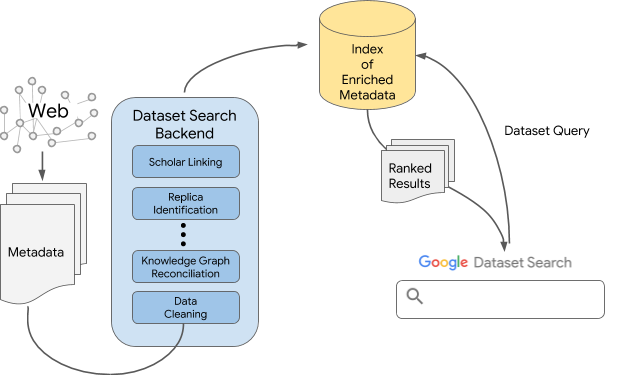
At a very high level, Google Data Search relies on dataset providers, big and small, adding structured metadata on their sites using the open schema.org/Dataset standard. The metadata specifies the salient properties of each dataset: its name and description, spatial and temporal coverage, provenance information, and so on. Dataset Search uses this metadata, links it with other resources that are available at Google (more on this below!), and builds an index of this enriched corpus of metadata. Once we built the index, we can start answering user queries — and figuring out which results best correspond to the query.
An overview of the technology behind Google Dataset Search
Using Structured Metadata from Data Providers
When Google's search engine processes a Web page with schema.org/Dataset mark-up, it understands that there is dataset metadata there and processes that structured metadata to create "records" describing each annotated dataset on a page. The use of schema.org allows developers to embed this structured information into HTML, without affecting the appearance of the page while making the semantics of the information visible to all search engines.

However, no matter how precise schema.org definitions or guidelines are, some metadata will inevitably be incomplete, wrong, or entirely missing. Furthermore, distinctions between some fields can be vague: is the dataset repository a publisher or a provider of a dataset? How do we distinguish between citations to a scientific paper that describes the creation of the dataset vs. papers describing its use? Indeed, many of these questions often generate active scholarly discussions.

Despite these variations, Dataset Search must provide a uniform and predictable user experience on the front end. Therefore, in some cases we substitute a more general field name (e.g., “provided by”) to display the values coming from multiple other fields (e.g., “publisher”, “creator”, etc.). In other cases, we are not able to use some of the fields at all: if a specific field is being misinterpreted in many different ways by dataset providers, we bypass that field for now and work with the community to clarify the guidelines. In each decision, we had one specific question that helped us in difficult cases "What will help data discovery the most?" This focus on the task that we were addressing made some of the problems easier than they seemed at first.

Connecting Replicas of Datasets
It is very common for a dataset, in particular a popular one, to be present in more than one repository. We use a variety of signals to determine when two datasets are replicas of each other. For example, schema.org has a way to specify the connection explicitly, through schema.org/sameAs, which is the best way to link different replicas together and to point to the canonical source of a dataset. Other signals include two datasets descriptions pointing to the same canonical page, having the same Digital Object Identifier (DOI), sharing links for downloading the dataset, or having a large overlap in other metadata fields. None of these signals are perfect in isolation, therefore we combine them to get the strongest possible indication of when two datasets are the same.

Reconciling to the Google Knowledge Graph
Google's Knowledge Graph is a powerful platform that describes and links information about many entities, including the ones that appear in dataset metadata: organizations providing datasets, locations for spatial coverage of the data, funding agencies, and so on. Therefore, we try to reconcile information mentioned in the metadata fields with the items in the Knowledge Graph. We can do this reconciliation with good precision for two main reasons. First, we know the types of items in the Knowledge Graph and the types of entities that we expect in the metadata fields. Therefore, we can limit the types of entities from the Knowledge Graph that we match with values for a particular metadata field. For example, a provider of a dataset should match with an organization entity in the Knowledge Graph and not with, say, a location. Second, the context of the Web page itself helps reduce the number of choices, which is particularly useful for distinguishing between organizations that share the same acronym. For example, the acronym CAMRA can stand for “Chilbolton Advanced Meteorological Radar” or “Campaign for Real Ale”. If we use terms from the Web page, we can then more easily determine that CAMRA is in fact the Chilbolton Radar when we see terms such as “clouds”, “vapor”, and “water” on the page.

This type of reconciliation opens up lots of possibilities to improve the search experience for users. For instance, Dataset Search can localize results by showing reconciled values of metadata in the same language as the rest of the page. Additionally, it can rely on synonyms, correct misspellings, expand acronyms, or use other relations in the Knowledge Graph for query expansion.

Linking to other Google Resources
Google has many other data resources that are useful in augmenting the dataset metadata, such as Google Scholar. Knowing which datasets are referenced and cited in publications serves at least two purposes:
  1. It provides a valuable signal about the importance and prominence of a dataset.
  2. It gives dataset authors an easy place to see citations to their data and to get credit.
Indeed, we hope that highlighting publications that use the data will lead to a more healthy ecosystem of data citation. For the moment, our links to Google scholar are very approximate as we lack a good model on how people cite data. We try to go beyond DOIs to give somewhat better coverage, but the number of articles citing a dataset ends up being approximate. We hope to make more progress in this area in order to get a higher level of precision.

Search and Ranking of Results
When a user issues a query, we search through the corpus of datasets, in a way not unlike Google Search works over Web pages. Just like with any search, we need to determine whether a document is relevant for the query and then rank the relevant documents. Because there are no large-scale studies on how users search for datasets, as a first approximation, we rely on Google Web ranking. However, ranking datasets is different from ranking Web pages, and we add some additional signals that take into account the metadata quality, citations, and so on. As Dataset Search gets used more by our users and we understand better how users search for datasets, we hope that ranking will improve significantly.

A Better Open Data Ecosystem
We built Dataset Search in an attempt to create a tool that will positively impact the discoverability of data. The decision to rely on open standards (schema.org, W3C DCAT, JSON-LD, etc.) for markup is intentional, as Dataset Search can only be as good as the open-data ecosystem that it supports. As such, Google Dataset Search aims to support a strong open data ecosystem by encouraging:
  1. Widespread adoption of open metadata formats to describe published data.
  2. Further development of open metadata formats to describe more types of data and in more detail.
  3. The culture of citing data the way we cite research publications, giving those who create and publish the data the credit that they deserve.
  4. The development of tools that leverage this metadata to enable more discovery or better use of data. 
The increased adoption of open metadata standards in conjunction with the continued development of Dataset Search (and, hopefully, other tools) should foster a healthier open data ecosystem where data is a first-class citizen of research.

So, Where is Your Dataset?
It is probably clear by now that Dataset Search is only as good as the metadata that exists on the Web pages for datasets. The most common answer to the question of why a specific dataset does not show up in our results is that the Web page for that dataset does not have any markup. Just pop that page into the Structured Data Testing Tool and you will see whether the markup is there. If you don't see any markup there, and you own the page, you can add it and if you don't own the page, you can ask the page owners to do it, which will make their page more easily discoverable by everyone.

We hope that the community finds Dataset Search useful, users make serendipitous discoveries and save time and scientists and journalists spend less time searching for data and more time using it.

Acknowledgements
We would like to thank Xiaomeng Ban, Dan Brickley, Lee Butler, Thomas Chen, Corinna Cortes, Kevin Espinoza, Archana Jain, Mike Jones, Kishore Papineni, Chris Sater, Gokhan Turhan, Shubin Zhao and Andi Vajda for their work on the project and all our partners, collaborators, and early adopters for their help.

Source: Google AI Blog


Machine Learning in Google BigQuery


Google BiqQuery allows interactive analysis of large datasets, making it easy for businesses to share meaningful insights and develop solutions based on customer analytics. However, many of the businesses that are using BigQuery aren’t using machine learning to help better understand the data they are generating. This is because data analysts, proficient in SQL, may not have the traditional data science background needed to apply machine learning techniques.

Today we’re announcing BigQuery ML, a capability inside BigQuery that allows data scientists and analysts to build and deploy machine learning models on massive structured or semi-structured datasets. BigQuery ML is a set of simple SQL language extensions which enables users to utilize popular ML capabilities, performing predictive analytics like forecasting sales and creating customer segmentations right at the source, where they already store their data. BigQuery ML additionally sets smart defaults automatically and takes care of data transformation, leading to a seamless and easy to use experience with great results.
When designing the BigQuery ML backend, the team was faced with a dilemma. Transferring large amounts of data from BigQuery servers to special-purpose servers running machine learning algorithms would be time-consuming and would incur an overhead in terms of security and privacy considerations. However, because the core components of gradient descent — an optimization method that is the workhorse of machine learning algorithms — can be implemented using common SQL operations*, we were able to repurpose the existing BigQuery SQL processing engine for BigQuery ML.

Since the BigQuery engine is designed to efficiently scan large datasets rather than randomly draw small samples from them, BigQuery ML is based on the standard (batch) variant of gradient descent rather than the stochastic version. And while stochastic gradient descent is far more common in today’s large-scale machine learning systems, the batch variant has numerous practical advantages.

For example, in-database machine learning systems based on stochastic gradient descent process examples one by one, and can perform poorly when the data is suboptimally ordered. But BigQuery data is often distributed on disk so as to optimize the performance of regular SQL queries, and continually redistributing the data to support stochastic machine learning algorithms would be computationally expensive. In contrast, batch gradient descent is insensitive to the ordering and partitioning of data on disk, thereby completely circumventing this problem. Also, batch methods can be combined with line search techniques from the classical optimization literature, leading to a learning algorithm that is more stable and requires less fine tuning. Using line search with stochastic methods is far trickier. Our implementation also includes support for regularization and preconditioning. For more details, please see our paper.

We hope that you’ll find BigQuery ML useful for many predictive analytics tasks. To try it, visit the BigQuery console and follow the user guide. Creating a model is as simple as:
CREATE MODEL dataset.model_name
OPTIONS(model_type=’linear_reg’, input_label_cols=[‘input_label’])
AS SELECT * FROM input_table;
In the future, we plan to further integrate our gradient descent implementation with BigQuery infrastructure to realize more performance gains. We’re also going to explore other machine learning algorithms that can be easily and efficiently implemented for large-scale problems by leveraging the power of BigQuery.

Acknowledgements
BigQuery ML is the result of a large collaboration across many teams at Google. Key contributors and sponsors include Hossein Ahmadi, Corinna Cortes, Grzegorz Czajkowski, Mingge Deng, Amir Hormati, Abhishek Kashyap, Jing Jing Long, Dan McClary, Chris Meyers, Girishkumar Sabhnani, Vivek Sharma, Jordan Tigani, Chad Verbowski, Jiaxun Wu and Lisa Yin.


* For example, a gradient vector can be computed using the SUM and GROUP BY operators, and the weights of a model can be updated using an INNER JOIN.

Source: Google AI Blog


Announcing the Google Cloud Platform Research Credits Program


Scientists across nearly every discipline are researching ever larger and more complex data sets, using tremendous amounts of compute power to learn, make discoveries and build new tools that few could have imagined only a few years ago. Traditionally, this kind of research has been limited by the availability of resources, with only the largest universities or industry partners able to successfully pursue these endeavors. However, the power of cloud computing has been removing obstacles that many researchers used to face, enabling projects that use machine learning tools to understand and address student questions and that study robotic interactions with humans, among many more.

In order to ensure that more researchers have access to powerful cloud tools, we’re launching Google Cloud Platform (GCP) research credits, a new program aimed to support faculty in qualified regions who want to take advantage of GCP’s compute, analytics, and machine-learning capabilities for research. Higher education researchers can use GCP research credits in a multitude of ways — below are just three examples to illustrate how GCP can help propel your research forward.

Andrew V. Sutherland, a computational number theorist and Principal Research Scientist at the Massachusetts Institute of Technology, is one of a growing number of academic researchers who has already made the transition and benefited from GCP. His team moved his extremely large database to GCP because “we are mathematicians who want to focus on our research, and not have to worry about hardware failures or scaling issues with the website.”

Ryan Abernathey, Assistant Professor of Earth and Environmental Sciences, Ocean and Climate Physics at the Lamont-Doherty Earth Observatory at Columbia University, used Google Cloud credits through an NSF partnership and, with his team, developed an open-source platform to manage the complex data sets of climate science. The platform, called Pangeo, can run Earth System Modeling simulations on petabytes of high-resolution, three-dimensional data. “This is the future of what day-to-day science research computing will look like,” he predicts.

At the Stanford Center for Genomics and Personalized Medicine (SCGPM), researchers using GCP and BigQuery can now run hundreds of genomes through a variant analysis pipeline and get query results quickly. Mike Snyder, director of SCGPM, notes, “We’re entering an era where people are working with thousands or tens of thousands or even million genome projects, and you’re never going to do that on a local cluster very easily. Cloud computing is where the field is going.”

The GCP research credits program is open to faculty doing cutting-edge research in eligible countries. We’re eager to hear how we can help accelerate your progress. If you’re interested, you can learn more on our website or apply now.

Source: Google AI Blog


Creating Custom Estimators in TensorFlow

Posted by the TensorFlow Team

Welcome to Part 3 of a blog series that introduces TensorFlow Datasets and Estimators. Part 1 focused on pre-made Estimators, while Part 2 discussed feature columns. Here in Part 3, you'll learn how to create your own custom Estimators. In particular, we're going to demonstrate how to create a custom Estimator that mimics DNNClassifier's behavior when solving the Iris problem.

If you are feeling impatient, feel free to compare and contrast the following full programs:

  • Source code for Iris implemented with the pre-made DNNClassifier Estimator here.
  • Source code for Iris implemented with the custom Estimator here.

Pre-made vs. custom

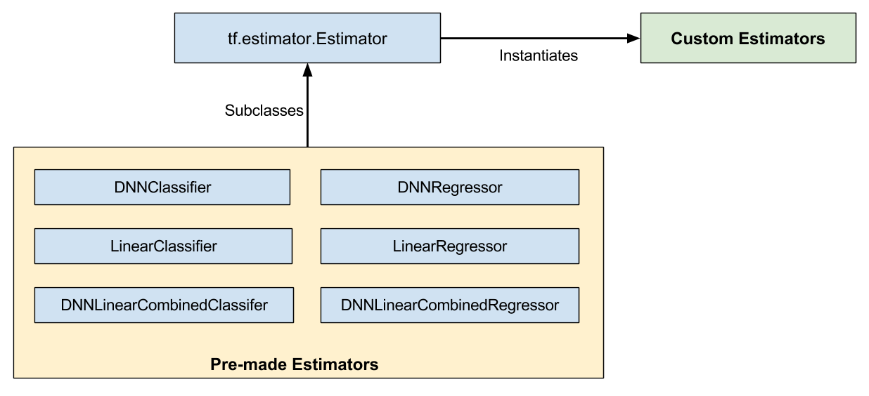
As Figure 1 shows, pre-made Estimators are subclasses of the tf.estimator.Estimatorbase class, while custom Estimators are an instantiation of tf.estimator.Estimator:

Figure 1. Pre-made and custom Estimators are all Estimators.

Pre-made Estimators are fully-baked. Sometimes though, you need more control over an Estimator's behavior. That's where custom Estimators come in.

You can create a custom Estimator to do just about anything. If you want hidden layers connected in some unusual fashion, write a custom Estimator. If you want to calculate a unique metric for your model, write a custom Estimator. Basically, if you want an Estimator optimized for your specific problem, write a custom Estimator.

A model function (model_fn) implements your model. The only difference between working with pre-made Estimators and custom Estimators is:

  • With pre-made Estimators, someone already wrote the model function for you.
  • With custom Estimators, you must write the model function.

Your model function could implement a wide range of algorithms, defining all sorts of hidden layers and metrics. Like input functions, all model functions must accept a standard group of input parameters and return a standard group of output values. Just as input functions can leverage the Dataset API, model functions can leverage the Layers API and the Metrics API.

Iris as a pre-made Estimator: A quick refresher

Before demonstrating how to implement Iris as a custom Estimator, we wanted to remind you how we implemented Iris as a pre-made Estimator in Part 1 of this series. In that Part, we created a fully connected, deepneural network for the Iris dataset simply by instantiating a pre-made Estimator as follows:

# Instantiate a deep neural network classifier.
classifier = tf.estimator.DNNClassifier(
feature_columns=feature_columns, # The input features to our model.
hidden_units=[10, 10], # Two layers, each with 10 neurons.
n_classes=3, # The number of output classes (three Iris species).
model_dir=PATH) # Pathname of directory where checkpoints, etc. are stored.

The preceding code creates a deep neural network with the following characteristics:

  • A list of feature columns. (The definitions of the feature columns are not shown in the preceding snippet.) For Iris, the feature columns are numeric representations of four input features.
  • Two fully connected layers, each having 10 neurons. A fully connected layer (also called a dense layer) is connected to every neuron in the subsequent layer.
  • An output layer consisting of a three-element list. The elements of that list are all floating-point values; the sum of those values must be 1.0 (this is a probability distribution).
  • A directory (PATH) in which the trained model and various checkpoints will be stored.

Figure 2 illustrates the input layer, hidden layers, and output layer of the Iris model. For reasons pertaining to clarity, we've only drawn 4 of the nodes in each hidden layer.

Figure 2. Our implementation of Iris contains four features, two hidden layers, and a logits output layer.

Let's see how to solve the same Iris problem with a custom Estimator.

Input function

One of the biggest advantages of the Estimator framework is that you can experiment with different algorithms without changing your data pipeline. We will therefore reuse much of the input function from Part 1:

def my_input_fn(file_path, repeat_count=1, shuffle_count=1):
def decode_csv(line):
parsed_line = tf.decode_csv(line, [[0.], [0.], [0.], [0.], [0]])
label = parsed_line[-1] # Last element is the label
del parsed_line[-1] # Delete last element
features = parsed_line # Everything but last elements are the features
d = dict(zip(feature_names, features)), label
return d

dataset = (tf.data.TextLineDataset(file_path) # Read text file
.skip(1) # Skip header row
.map(decode_csv, num_parallel_calls=4) # Decode each line
.cache() # Warning: Caches entire dataset, can cause out of memory
.shuffle(shuffle_count) # Randomize elems (1 == no operation)
.repeat(repeat_count) # Repeats dataset this # times
.batch(32)
.prefetch(1) # Make sure you always have 1 batch ready to serve
)
iterator = dataset.make_one_shot_iterator()
batch_features, batch_labels = iterator.get_next()
return batch_features, batch_labels

Notice that the input function returns the following two values:

  • batch_features, which is a dictionary. The dictionary's keys are the names of the features, and the dictionary's values are the feature's values.
  • batch_labels, which is a list of the label's values for a batch.

Refer to Part 1 for full details on input functions.

Create feature columns

As detailed in Part 2 of our series, you must define your model's feature columns to specify the representation of each feature. Whether working with pre-made Estimators or custom Estimators, you define feature columns in the same fashion. For example, the following code creates feature columns representing the four features (all numerical) in the Iris dataset:

feature_columns = [
tf.feature_column.numeric_column(feature_names[0]),
tf.feature_column.numeric_column(feature_names[1]),
tf.feature_column.numeric_column(feature_names[2]),
tf.feature_column.numeric_column(feature_names[3])
]

Write a model function

We are now ready to write the model_fn for our custom Estimator. Let's start with the function declaration:

def my_model_fn(
features, # This is batch_features from input_fn
labels, # This is batch_labels from input_fn
mode): # Instance of tf.estimator.ModeKeys, see below

The first two arguments are the features and labels returned from the input function; that is, features and labels are the handles to the data your model will use. The mode argument indicates whether the caller is requesting training, predicting, or evaluating.

To implement a typical model function, you must do the following:

  • Define the model's layers.
  • Specify the model's behavior in three the different modes.

Define the model's layers

If your custom Estimator generates a deep neural network, you must define the following three layers:

  • an input layer
  • one or more hidden layers
  • an output layer

Use the Layers API (tf.layers) to define hidden and output layers.

If your custom Estimator generates a linear model, then you only have to generate a single layer, which we'll describe in the next section.

Define the input layer

Call tf.feature_column.input_layerto define the input layer for a deep neural network. For example:

# Create the layer of input
input_layer = tf.feature_column.input_layer(features, feature_columns)

The preceding line creates our input layer, reading our featuresthrough the input function and filtering them through the feature_columns defined earlier. See Part 2 for details on various ways to represent data through feature columns.

To create the input layer for a linear model, call tf.feature_column.linear_modelinstead of tf.feature_column.input_layer. Since a linear model has no hidden layers, the returned value from tf.feature_column.linear_model serves as both the input layer and output layer. In other words, the returned value from this function isthe prediction.

Establish Hidden Layers

If you are creating a deep neural network, you must define one or more hidden layers. The Layers API provides a rich set of functions to define all types of hidden layers, including convolutional, pooling, and dropout layers. For Iris, we're simply going to call tf.layers.Densetwice to create two dense hidden layers, each with 10 neurons. By "dense," we mean that each neuron in the first hidden layer is connected to each neuron in the second hidden layer. Here's the relevant code:

# Definition of hidden layer: h1
# (Dense returns a Callable so we can provide input_layer as argument to it)
h1 = tf.layers.Dense(10, activation=tf.nn.relu)(input_layer)

# Definition of hidden layer: h2
# (Dense returns a Callable so we can provide h1 as argument to it)
h2 = tf.layers.Dense(10, activation=tf.nn.relu)(h1)

The inputs parameter to tf.layers.Dense identifies the preceding layer. The layer preceding h1 is the input layer.

Figure 3. The input layer feeds into hidden layer 1.

The preceding layer to h2 is h1. So, the string of layers now looks like this:

Figure 4. Hidden layer 1 feeds into hidden layer 2.

The first argument to tf.layers.Densedefines the number of its output neurons—10 in this case.

The activation parameter defines the activation function—Relu in this case.

Note that tf.layers.Denseprovides many additional capabilities, including the ability to set a multitude of regularization parameters. For the sake of simplicity, though, we're going to simply accept the default values of the other parameters. Also, when looking at tf.layersyou may encounter lower-case versions (e.g. tf.layers.dense). As a general rule, you should use the class versions which start with a capital letter (tf.layers.Dense).

Output Layer

We'll define the output layer by calling tf.layers.Dense yet again:

# Output 'logits' layer is three numbers = probability distribution
# (Dense returns a Callable so we can provide h2 as argument to it)
logits = tf.layers.Dense(3)(h2)

Notice that the output layer receives its input from h2. Therefore, the full set of layers is now connected as follows:

Figure 5. Hidden layer 2 feeds into the output layer.

When defining an output layer, the units parameter specifies the number of possible output values. So, by setting units to 3, the tf.layers.Densefunction establishes a three-element logits vector. Each cell of the logits vector contains the probability of the Iris being Setosa, Versicolor, or Virginica, respectively.

Since the output layer is a final layer, the call to tf.layers.Denseomits the optional activation parameter.

Implement training, evaluation, and prediction

The final step in creating a model function is to write branching code that implements prediction, evaluation, and training.

The model function gets invoked whenever someone calls the Estimator's train, evaluate, or predict methods. Recall that the signature for the model function looks like this:

def my_model_fn(
features, # This is batch_features from input_fn
labels, # This is batch_labels from input_fn
mode): # Instance of tf.estimator.ModeKeys, see below

Focus on that third argument, mode. As the following table shows, when someone calls train, evaluate, or predict, the Estimator framework invokes your model function with the mode parameter set as follows:

Table 2. Values of mode.

Caller invokes custom Estimator method... Estimator framework calls your model function with the mode parameter set to...
train() ModeKeys.TRAIN
evaluate() ModeKeys.EVAL
predict() ModeKeys.PREDICT

For example, suppose you instantiate a custom Estimator to generate an object named classifier. Then, you might make the following call (never mind the parameters to my_input_fn at this time):

classifier.train(
input_fn=lambda: my_input_fn(FILE_TRAIN, repeat_count=500, shuffle_count=256))

The Estimator framework then calls your model function with mode set to ModeKeys.TRAIN.

Your model function must provide code to handle all three of the mode values. For each mode value, your code must return an instance of tf.estimator.EstimatorSpec, which contains the information the caller requires. Let's examine each mode.

PREDICT

When model_fn is called with mode == ModeKeys.PREDICT, the model function must return a tf.estimator.EstimatorSpeccontaining the following information:

  • the mode, which is tf.estimator.ModeKeys.PREDICT
  • the prediction

The model must have been trained prior to making a prediction. The trained model is stored on disk in the directory established when you instantiated the Estimator.

For our case, the code to generate the prediction looks as follows:

# class_ids will be the model prediction for the class (Iris flower type)
# The output node with the highest value is our prediction
predictions = { 'class_ids': tf.argmax(input=logits, axis=1) }

# Return our prediction
if mode == tf.estimator.ModeKeys.PREDICT:
return tf.estimator.EstimatorSpec(mode, predictions=predictions)

The block is surprisingly brief--the lines of code are simply the bucket at the end of a long hose that catches the falling predictions. After all, the Estimator has already done all the heavy lifting to make a prediction:

  1. The input function provides the model function with data (feature values) to infer from.
  2. The model function transforms those feature values into feature columns.
  3. The model function runs those feature columns through the previously-trained model.

The output layer is a logits vector that contains the value of each of the three Iris species being the input flower. The tf.argmaxmethod selects the Iris species in that logits vector with the highest value.

Notice that the highest value is assigned to a dictionary key named class_ids. We return that dictionary through the predictions parameter of tf.estimator.EstimatorSpec. The caller can then retrieve the prediction by examining the dictionary passed back to the Estimator's predict method.

EVAL

When model_fn is called with mode == ModeKeys.EVAL, the model function must evaluate the model, returning loss and possibly one or more metrics.

We can calculate loss by calling tf.losses.sparse_softmax_cross_entropy. Here's the complete code:

# To calculate the loss, we need to convert our labels
# Our input labels have shape: [batch_size, 1]
labels = tf.squeeze(labels, 1) # Convert to shape [batch_size]
loss = tf.losses.sparse_softmax_cross_entropy(labels=labels, logits=logits)

Now let's turn our attention to metrics. Although returning metrics is optional, most custom Estimators return at least one metric. TensorFlow provides a Metrics API (tf.metrics) to calculate different kinds of metrics. For brevity's sake, we'll only return accuracy. The tf.metrics.accuracycompares our predictions against the "true labels", that is, against the labels provided by the input function. The tf.metrics.accuracyfunction requires the labels and predictions to have the same shape (which we did earlier). Here's the call to tf.metrics.accuracy:

# Calculate the accuracy between the true labels, and our predictions
accuracy = tf.metrics.accuracy(labels, predictions['class_ids'])

When the model is called with mode == ModeKeys.EVAL, the model function returns a tf.estimator.EstimatorSpec containing the following information:

  • the mode, which is tf.estimator.ModeKeys.EVAL
  • the model's loss
  • typically, one or more metrics encased in a dictionary.

So, we'll create a dictionary containing our sole metric (my_accuracy). If we had calculated other metrics, we would have added them as additional key/value pairs to that same dictionary. Then, we'll pass that dictionary in the eval_metric_ops argument of tf.estimator.EstimatorSpec. Here's the block:

# Return our loss (which is used to evaluate our model)
# Set the TensorBoard scalar my_accurace to the accuracy
# Obs: This function only sets value during mode == ModeKeys.EVAL
# To set values during training, see tf.summary.scalar
if mode == tf.estimator.ModeKeys.EVAL:
return tf.estimator.EstimatorSpec(
mode,
loss=loss,
eval_metric_ops={'my_accuracy': accuracy})

TRAIN

When model_fn is called with mode == ModeKeys.TRAIN, the model function must train the model.

We must first instantiate an optimizer object. We picked Adagrad (tf.train.AdagradOptimizer) in the following code block only because we're mimicking the DNNClassifier, which also uses Adagrad. The tf.trainpackage provides many other optimizers—feel free to experiment with them.

Next, we train the model by establishing an objective on the optimizer, which is simply to minimize its loss. To establish that objective, we call the minimizemethod.

In the code below, the optional global_step argument specifies the variable that TensorFlow uses to count the number of batches that have been processed. Setting global_step to tf.train.get_global_stepwill work beautifully. Also, we are calling tf.summary.scalarto report my_accuracy to TensorBoard during training. For both of these notes, please see the section on TensorBoard below for further explanation.

optimizer = tf.train.AdagradOptimizer(0.05)
train_op = optimizer.minimize(
loss,
global_step=tf.train.get_global_step())

# Set the TensorBoard scalar my_accuracy to the accuracy
tf.summary.scalar('my_accuracy', accuracy[1])

When the model is called with mode == ModeKeys.TRAIN, the model function must return a tf.estimator.EstimatorSpeccontaining the following information:

  • the mode, which is tf.estimator.ModeKeys.TRAIN
  • the loss
  • the result of the training op

Here's the code:

# Return training operations: loss and train_op
return tf.estimator.EstimatorSpec(
mode,
loss=loss,
train_op=train_op)

Our model function is now complete!

The custom Estimator

After creating your new custom Estimator, you'll want to take it for a ride. Start by

instantiating the custom Estimator through the Estimatorbase class as follows:

classifier = tf.estimator.Estimator(
model_fn=my_model_fn,
model_dir=PATH) # Path to where checkpoints etc are stored

The rest of the code to train, evaluate, and predict using our estimator is the same as for the pre-made DNNClassifierdescribed in Part 1. For example, the following line triggers training the model:

classifier.train(
input_fn=lambda: my_input_fn(FILE_TRAIN, repeat_count=500, shuffle_count=256))

TensorBoard

As in Part 1, we can view some training results in TensorBoard. To see this reporting, start TensorBoard from your command-line as follows:

# Replace PATH with the actual path passed as model_dir
tensorboard --logdir=PATH

Then browse to the following URL:

localhost:6006 

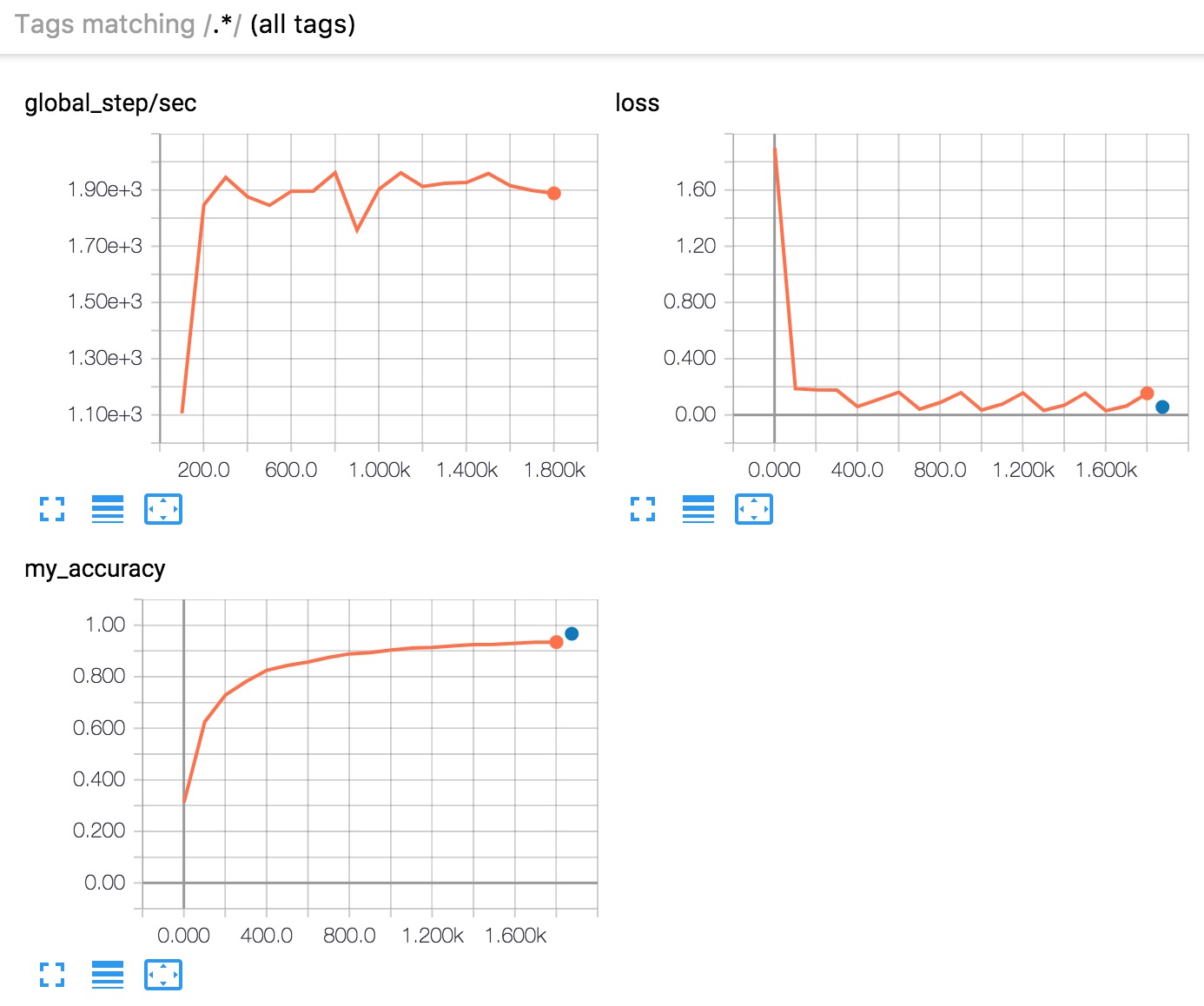
All the pre-made Estimators automatically log a lot of information to TensorBoard. With custom Estimators, however, TensorBoard only provides one default log (a graph of loss) plus the information we explicitly tell TensorBoard to log. Therefore, TensorBoard generates the following from our custom Estimator:

Figure 6. TensorBoard displays three graphs.

In brief, here's what the three graphs tell you:

  • global_step/sec: A performance indicator, showing how many batches (gradient updates) we processed per second (y-axis) at a particular batch (x-axis). In order to see this report, you need to provide a global_step (as we did with tf.train.get_global_step()). You also need to run training for a sufficiently long time, which we do by asking the Estimator train for 500 epochs when we call its train method:
    • loss: The loss reported. The actual loss value (y-axis) doesn't mean much. The shape of the graph is what's important.
  • my_accuracy: The accuracy recorded when we invoked both of the following:
  • eval_metric_ops={'my_accuracy': accuracy}), during EVAL (when returning our EstimatorSpec)
  • tf.summary.scalar('my_accuracy', accuracy[1]), during TRAIN

Note the following in the my_accuracy and loss graphs:

  • The orange line represents TRAIN.
  • The blue dot represents EVAL.

During TRAIN, orange values are recorded continuously as batches are processed, which is why it becomes a graph spanning x-axis range. By contrast, EVAL produces only a single value from processing all the evaluation steps.

As suggested in Figure 7, you may see and also selectively disable/enable the reporting for training and evaluation the left side. (Figure 7 shows that we kept reporting on for both:)

Figure 7. Enable or disable reporting.

In order to see the orange graph, you must specify a global step. This, in combination with getting global_steps/sec reported, makes it a best practice to always register a global step by passing tf.train.get_global_step()as an argument to the optimizer.minimize call.

Summary

Although pre-made Estimators can be an effective way to quickly create new models, you will often need the additional flexibility that custom Estimators provide. Fortunately, pre-made and custom Estimators follow the same programming model. The only practical difference is that you must write a model function for custom Estimators. Everything else is the same!

For more details, be sure to check out:

Until next time - Happy TensorFlow coding!