Tag Archives: datasets

Advancing Instance-Level Recognition Research

Instance-level recognition (ILR) is the computer vision task of recognizing a specific instance of an object, rather than simply the category to which it belongs. For example, instead of labeling an image as “post-impressionist painting”, we’re interested in instance-level labels like “Starry Night Over the Rhone by Vincent van Gogh”, or “Arc de Triomphe de l'Étoile, Paris, France”, instead of simply “arch”. Instance-level recognition problems exist in many domains, like landmarks, artwork, products, or logos, and have applications in visual search apps, personal photo organization, shopping and more. Over the past several years, Google has been contributing to research on ILR with the Google Landmarks Dataset and Google Landmarks Dataset v2 (GLDv2), and novel models such as DELF and Detect-to-Retrieve.

Three types of image recognition problems, with different levels of label granularity (basic, fine-grained, instance-level), for objects from the artwork, landmark and product domains. In our work, we focus on instance-level recognition.

Today, we highlight some results from the Instance-Level Recognition Workshop at ECCV’20. The workshop brought together experts and enthusiasts in this area, with many fruitful discussions, some of which included our ECCV’20 paper “DEep Local and Global features” (DELG), a state-of-the-art image feature model for instance-level recognition, and a supporting open-source codebase for DELG and other related ILR techniques. Also presented were two new landmark challenges (on recognition and retrieval tasks) based on GLDv2, and future ILR challenges that extend to other domains: artwork recognition and product retrieval. The long-term goal of the workshop and challenges is to foster advancements in the field of ILR and push forward the state of the art by unifying research workstreams from different domains, which so far have mostly been tackled as separate problems.

DELG: DEep Local and Global Features
Effective image representations are the key components required to solve instance-level recognition problems. Often, two types of representations are necessary: global and local image features. A global feature summarizes the entire contents of an image, leading to a compact representation but discarding information about spatial arrangement of visual elements that may be characteristic of unique examples. Local features, on the other hand, comprise descriptors and geometry information about specific image regions; they are especially useful to match images depicting the same objects.

Currently, most systems that rely on both of these types of features need to separately adopt each of them using different models, which leads to redundant computations and lowers overall efficiency. To address this, we proposed DELG, a unified model for local and global image features.

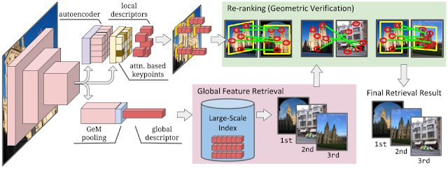
The DELG model leverages a fully-convolutional neural network with two different heads: one for global features and the other for local features. Global features are obtained using pooled feature maps of deep network layers, which in effect summarize the salient features of the input images making the model more robust to subtle changes in input. The local feature branch leverages intermediate feature maps to detect salient image regions, with the help of an attention module, and to produce descriptors that represent associated localized contents in a discriminative manner.

Our proposed DELG model (left). Global features can be used in the first stage of a retrieval-based system, to efficiently select the most similar images (bottom). Local features can then be employed to re-rank top results (top, right), increasing the precision of the system.

This novel design allows for efficient inference since it enables extraction of global and local features within a single model. For the first time, we demonstrated that such a unified model can be trained end-to-end and deliver state-of-the-art results for instance-level recognition tasks. When compared to previous global features, this method outperforms other approaches by up to 7.5% mean average precision; and for the local feature re-ranking stage, DELG-based results are up to 7% better than previous work. Overall, DELG achieves 61.2% average precision on the recognition task of GLDv2, which outperforms all except two methods of the 2019 challenge. Note that all top methods from that challenge used complex model ensembles, while our results use only a single model.

Tensorflow 2 Open-Source Codebase
To foster research reproducibility, we are also releasing a revamped open-source codebase that includes DELG and other techniques relevant to instance-level recognition, such as DELF and Detect-to-Retrieve. Our code adopts the latest Tensorflow 2 releases, and makes available reference implementations for model training & inference, besides image retrieval and matching functionalities. We invite the community to use and contribute to this codebase in order to develop strong foundations for research in the ILR field.

New Challenges for Instance Level Recognition
Focused on the landmarks domain, the Google Landmarks Dataset v2 (GLDv2) is the largest available dataset for instance-level recognition, with 5 million images spanning 200 thousand categories. By training landmark retrieval models on this dataset, we have demonstrated improvements of up to 6% mean average precision, compared to models trained on earlier datasets. We have also recently launched a new browser interface for visually exploring the GLDv2 dataset.

This year, we also launched two new challenges within the landmark domain, one focusing on recognition and the other on retrieval. These competitions feature newly-collected test sets, and a new evaluation methodology: instead of uploading a CSV file with pre-computed predictions, participants have to submit models and code that are run on Kaggle servers, to compute predictions that are then scored and ranked. The compute restrictions of this environment put an emphasis on efficient and practical solutions.

The challenges attracted over 1,200 teams, a 3x increase over last year, and participants achieved significant improvements over our strong DELG baselines. On the recognition task, the highest scoring submission achieved a relative increase of 43% average precision score and on the retrieval task, the winning team achieved a 59% relative improvement of the mean average precision score. This latter result was achieved via a combination of more effective neural networks, pooling methods and training protocols (see more details on the Kaggle competition site).

In addition to the landmark recognition and retrieval challenges, our academic and industrial collaborators discussed their progress on developing benchmarks and competitions in other domains. A large-scale research benchmark for artwork recognition is under construction, leveraging The Met’s Open Access image collection, and with a new test set consisting of guest photos exhibiting various photometric and geometric variations. Similarly, a new large-scale product retrieval competition will capture various challenging aspects, including a very large number of products, a long-tailed class distribution and variations in object appearance and context. More information on the ILR workshop, including slides and video recordings, is available on its website.

With this research, open source code, data and challenges, we hope to spur progress in instance-level recognition and enable researchers and machine learning enthusiasts from different communities to develop approaches that generalize across different domains.

Acknowledgements
The main Google contributors of this project are André Araujo, Cam Askew, Bingyi Cao, Jack Sim and Tobias Weyand. We’d like to thank the co-organizers of the ILR workshop Ondrej Chum, Torsten Sattler, Giorgos Tolias (Czech Technical University), Bohyung Han (Seoul National University), Guangxing Han (Columbia University), Xu Zhang (Amazon), collaborators on the artworks dataset Nanne van Noord, Sarah Ibrahimi (University of Amsterdam), Noa Garcia (Osaka University), as well as our collaborators from the Metropolitan Museum of Art: Jennie Choi, Maria Kessler and Spencer Kiser. For the open-source Tensorflow codebase, we’d like to thank the help of recent contributors: Dan Anghel, Barbara Fusinska, Arun Mukundan, Yuewei Na and Jaeyoun Kim. We are grateful to Will Cukierski, Phil Culliton, Maggie Demkin for their support with the landmarks Kaggle competitions. Also we’d like to thank Ralph Keller and Boris Bluntschli for their help with data collection.

Source: Google AI Blog


An Analysis of Online Datasets Using Dataset Search (Published, in Part, as a Dataset)

There are tens of millions of datasets on the web, with content ranging from sensor data and government records, to results of scientific experiments and business reports. Indeed, there are datasets for almost anything one can imagine, be it diets of emperor penguins or where remote workers live. More than two years ago, we undertook an effort to design a search engine that would provide a single entry point to these millions of datasets and thousands of repositories. The result is Dataset Search, which we launched in beta in 2018 and fully launched in January 2020. In addition to facilitating access to data, Dataset Search reconciles and indexes datasets using the metadata descriptions that come directly from the dataset web pages using schema.org structure.

As of today, the complete Dataset Search corpus contains more than 31 million datasets from more than 4,600 internet domains. About half of these datasets come from .com domains, but .org and governmental domains are also well represented. The graph below shows the growth of the corpus over the last two years, and while we still don’t know what fraction of datasets on the web are currently in Dataset Search, the number continues to grow steadily.

Growth in the number of datasets indexed by Dataset Search

To better understand the breadth and utility of the datasets made available through Dataset Search, we published “Google Dataset Search by the Numbers”, accepted at the 2020 International Semantic Web Conference. Here we provide an overview of the available datasets, present metrics and insights originating from their analysis, and suggest best practices for publishing future scientific datasets. In order to enable other researchers to build analysis and tools using the metadata, we are also making a subset of the data publicly available.

A Range of Dataset Topics
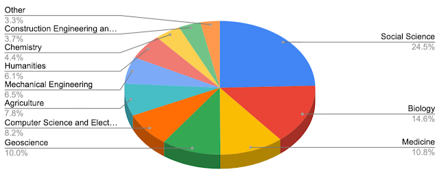
In order to determine the distribution of topics covered by the datasets, we infer the research category based on dataset titles and descriptions, as well as other text on the dataset Web pages. The two most common topics are geosciences and social sciences, which account for roughly 45% of the datasets. Biology is a close third at ~15%, followed by a roughly even distribution for other topics, including computer science, agriculture, and chemistry, among others.

Distribution of dataset topics

In our initial efforts to launch Dataset Search, we reached out to specific communities, which was key to bootstrapping widespread use of the corpus. Initially, we focused on geosciences and social sciences, but since then, we have allowed the corpus to grow organically. We were surprised to see that the fields associated with the communities we reached out to early on are still dominating the corpus. While their early involvement certainly contributes to their prevalence, there may be other factors involved, such as differences in culture across communities. For instance, geosciences have been particularly successful in making their data findable, accessible, interoperable, and reusable (FAIR), a core component to reducing barriers for access.

Making Data Easily Citable and Reusable
There is a growing consensus among researchers across scientific disciplines that it is important to make datasets available, to publish details relevant to their use, and to cite them when they are used. Many funding agencies and academic publishers require proper publication and citation of data.

Peer-reviewed journals such as Nature Scientific Data are dedicated to publishing valuable datasets, and efforts such as DataCite provide digital object identifiers (DOIs) for them. Resolution services (e.g., identifiers.org) also provide persistent, de-referenceable identifiers, allowing for easy citation, which is key to making datasets widely available in scientific discourse. Unfortunately, we found that only about 11% of the datasets in the corpus (or ~3M) have DOIs. We chose this subset from the dataset corpus to be included in our open-source release. From this collection, about 2.3M datasets come from two sites, datacite.org and figshare.com:

Domain Datasets with DOIs
figshare.com 1,301K
datacite.org 1,070K
narcis.nl 118K
openaire.eu 100K
datadiscoverystudio.org 72K
osti.gov 63K
zenodo.org 50K
researchgate.net 41K
da-ra.de 40K

Publishers can specify access requirements for a dataset via schema.org metadata properties, including details of the license and information indicating whether or not the dataset is accessible for free. Only 34% of datasets specify license information, but when no license is specified, users cannot make any assumptions on whether or not they are allowed to reuse the data. Thus, adding licensing information, and, ideally, adding as open a license as possible, will greatly improve the reusability of the data.

Among the datasets that did specify a license, we were able to recognize a known license in 72% of cases. Those licenses include Open Government licenses for the UK and Canada, Creative Commons licenses, and several Public Domain licenses (e.g., Public Domain Mark 1.0). We found 89.5% of these datasets to either be accessible for free or use a license that allows redistribution, or both. And of these open datasets, 5.6M (91%) allow commercial reuse.

Another critical component of data reusability is providing downloadable data, yet only 44% of datasets specify download information in their metadata. A possible explanation for this surprisingly low value is that webmasters (or dataset-hosting platforms) fear that exposing the data download link through schema.org metadata may lead search engines or other applications to give their users direct access to download the data, thus “stealing” traffic from their website. Another concern may be that data needs the proper context to be used appropriately (e.g., methodology, footnotes, and license information), and providers feel that only their web pages can give the complete picture. In Dataset Search, we do not show download links as part of dataset metadata so that users must go to the publisher’s website to download the data, where they will see the full context for the dataset.

What Do Users Access?
Finally, we examine how Dataset Search is being used. Overall, 2.1M unique datasets from 2.6K domains appeared in the top 100 Dataset Search results over 14 days in May 2020. We find that the distribution of topics being queried is different from that of the corpus as a whole. For instance, geoscience takes up a much smaller fraction, and conversely, biology and medicine represent a larger fraction relative to their share of the corpus. This result is likely explained by the timing of our analysis, as it was performed during the first weeks of the COVID-19 pandemic.

Distribution of topics covered by datasets that appear in search results

Best Practices for Publishing Scientific Datasets
Based on our analysis, we have identified a set of best practices that can improve how datasets are discovered, reused and cited.

  • Discoverability
    Dataset metadata should be on pages that are accessible to web crawlers and that provide metadata in machine-readable formats in order to improve discoverability.

  • Persistence
    Publishing metadata on sites that are likely to be more persistent than personal web pages will facilitate data reuse and citation. Indeed, during our analysis of Dataset Search, we noted a very high rate of turnover — many URLs that hosted a dataset one day did not have it a few weeks or months later. Data repositories, such as Figshare, Zenodo, DataDryad, Kaggle Datasets and many others, are a good way to ensure dataset persistence. Many of these repositories have agreements with libraries to preserve data in perpetuity.

  • Provenance
    With datasets often published in multiple repositories, it would be useful for repositories to describe the provenance information more explicitly in the metadata. The provenance information helps users understand who collected the data, where the primary source of the dataset is, or how it might have changed.

  • Licensing
    Datasets should include licensing information, ideally in a machine-readable format. Our analysis indicates that when dataset providers select a license, they tend to choose a fairly open one. So, encouraging and enabling scientists to choose licenses for their data will result in many more datasets being openly available.

  • Assigning persistent identifiers (such as DOIs)
    DOIs are critical for long-term tracking and useability. Not only do these identifiers allow for much easier citation of datasets and version tracking, they are also dereferenceable: if a dataset moves, the identifier can point to a different location.

Releasing Metadata for Datasets with Persistent Identifiers
As part of the announcement today, we are also releasing a subset of our corpus for others to use. It contains the metadata for more than three million datasets that have DOIs and other types of persistent identifiers –- these are the datasets that are the most easily citable. Researchers can use this metadata to perform deeper analysis or to build their own applications using this data. For example, much of the growth of DOI usage appears to have been within the last decade. How does this timeframe relate to the datasets covered in the corpus? Is the DOI usage distribution uniform across datasets, or are there significant differences between research communities?

We will update the dataset on a regular basis. Finally, we hope that focusing this data release on datasets with persistent citable identifiers will encourage more data providers to describe their datasets in more detail and to make them more easily citable.

In conclusion, we hope that having data more discoverable through tools such as Google's Dataset Search will encourage scientists to share their data more broadly and do it in a way that makes data truly FAIR.

Acknowledgments
This post reflects the work of the entire Dataset Search team. We are grateful to Shiyu Chen, Dimitris Paparas, Katrina Sostek, Yale Cong, Marc Najork, and Chris Gorgolewski for their contributions. We would also like to thank Hal Varian for suggesting this analysis and for many helpful ideas.

Source: Google AI Blog


Tackling Open Challenges in Offline Reinforcement Learning

Over the past several years, there has been a surge of interest in reinforcement learning (RL) driven by its high-profile successes in game playing and robotic control. However, unlike supervised learning methods, which learn from massive datasets that are collected once and then reused, RL algorithms use a trial-and-error feedback loop that requires active interaction during learning, collecting data every time a new policy is learned. This approach is prohibitive in many real-world settings, such as healthcare, autonomous driving, and dialogue systems, where trial-and-error data collection can be costly, time consuming, or even irresponsible. Even for problems where some active data collection can be used, the requirement for interactive collection limits dataset size and diversity.

Offline RL (also called batch RL or fully off-policy RL) relies solely on a previously collected dataset without further interaction. It provides a way to utilize previously collected datasets — from previous RL experiments, from human demonstrations, and from hand-engineered exploration strategies — in order to automatically learn decision-making strategies. In principle, while off-policy RL algorithms can be used in the offline setting (fully off-policy), they are generally only successful when used with active environment interaction — without receiving this direct feedback, they often exhibit undesirable performance in practice. Consequently, while offline RL has enormous potential, that potential cannot be reached without resolving significant algorithmic challenges.

In “Offline Reinforcement Learning: Tutorial, Review, and Perspectives on Open Problems”, we provide a comprehensive tutorial on approaches for tackling the challenges of offline RL and discuss the many issues that remain. To address these issues, we have designed and released an open-source benchmarking framework, Datasets for Deep Data-Driven Reinforcement Learning (D4RL), as well as a new, simple, and highly effective offline RL algorithm, called conservative Q-learning (CQL).

Benchmarks for Offline RL
In order to understand the capabilities of current approaches and to guide future progress, it is first necessary to have effective benchmarks. A common choice in prior work was to simply use data generated by a successful online RL run. However, while simple, this data collection approach is artificial because it involves training an online RL agent which is prohibitive in many real-world settings as we discussed previously. One wishes to learn a policy that is better than the current best from diverse data sources that provides good coverage of the task. For example, one might have data collected from a hand-designed controller of a robot arm, and use offline RL to train an improved controller. To enable progress in this field under realistic settings, one needs a benchmark suite that accurately reflects these settings, while being simple and accessible enough to enable rapid experimentation.

D4RL provides standardized environments, datasets and evaluation protocols, as well as reference scores for recent algorithms to help accomplish this. This is a “batteries-included” resource, making it ideal for anyone to jump in and get started with minimal fuss.

Environments in D4RL

The key design goal for D4RL was to develop tasks that reflect both real-world dataset challenges as well as real-world applications. Previous datasets used data collected either from random agents or agents trained with RL. Instead, by thinking through potential applications in autonomous driving, robotics, and other domains, we considered how real-world applications of offline RL might require handling of data generated from human demonstrations or hard-coded controllers, data collected from heterogeneous sources, and data collected by agents with a variety of different goals.

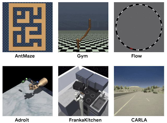
Aside from the widely used MuJoCo locomotion tasks, D4RL includes datasets for more complex tasks. The Adroit domain, which requires manipulating a realistic robotic hand to use a hammer, for example, illustrates the challenges of working with limited human demonstrations, without which these tasks are extremely challenging. Previous work found that existing datasets could not distinguish between competing methods, whereas the Adroit domain reveals clear deficiencies between them.

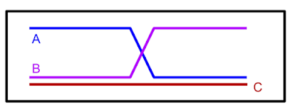
Another common scenario for real-world tasks is one in which the dataset used for training is collected from agents performing a wide range of other activities that are related to, but not specifically targeted towards, the task of interest. For example, data from human drivers may illustrate how to drive a car well, but do not necessarily show how to reach a specific desired destination. In this case, one might like offline RL methods to “stitch” together parts of routes in the driving dataset to accomplish a task that was not actually seen in the data (i.e., navigation). As an illustrative example, given paths labeled “A” and “B” in the picture below, offline RL should be able to “remix” them to produce path C.

Having only observed paths A and B, they can be combined to form a shortest path (C).

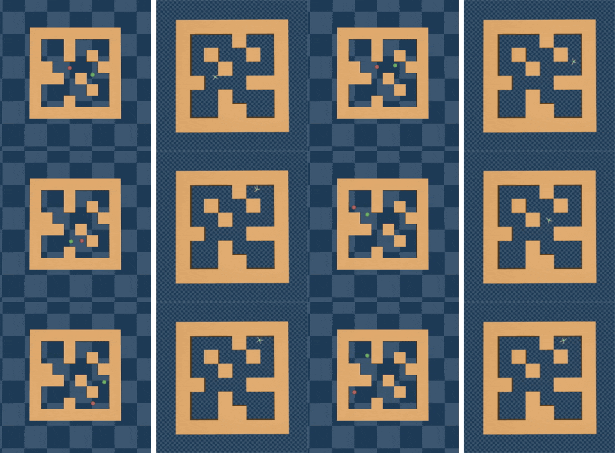
We constructed a series of increasingly difficult tasks to exercise this “stitching” ability. The maze environments, shown below, require two robots (a simple ball or an “Ant” robot) to navigate to locations in a series of mazes.

Maze navigation environments in D4RL, which require “stitching” parts of paths to accomplish new navigational goals that were not seen in the dataset.

A more complex “stitching” scenario is provided by the Franka kitchen domain (based on the Adept environment), where demonstrations from humans using a VR interface comprise a multi-task dataset, and offline RL methods must again “remix” this data.

The “Franka kitchen” domain requires using data from human demonstrators performing a variety of different tasks in a simulated kitchen.

Finally, D4RL includes two tasks that are meant to more accurately reflect potential realistic applications of offline RL, both based on existing driving simulators. One is a first-person driving dataset that utilizes the widely used CARLA simulator developed at Intel, which provides photo-realistic images in realistic driving domains, and the other is a dataset from the Flow traffic control simulator (from UC Berkeley), which requires controlling autonomous vehicles to facilitate effective traffic flow.

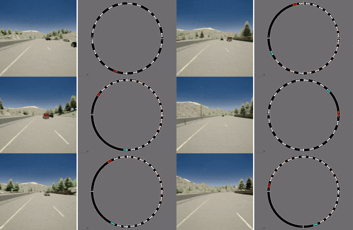
D4RL includes datasets based on existing realistic simulators for driving with CARLA (left) and traffic management with Flow (right).

We have packaged these tasks and standardized datasets into an easy-to-use Python package to accelerate research. Furthermore, we provide benchmark numbers for all tasks using relevant prior methods (BC, SAC, BEAR, BRAC, AWR, BCQ), in order to baseline new approaches. We are not the first to propose a benchmark for offline RL: a number of prior works have proposed simple datasets based on running RL algorithms, and several more recent works have proposed datasets with image observations and other features. However, we believe that the more realistic dataset composition in D4RL makes it an effective way to drive progress in the field.

An Improved Algorithm for Offline RL
As we developed the benchmark tasks, we found that existing methods could not solve the more challenging tasks. The central challenge arises from a distributional shift: in order to improve over the historical data, offline RL algorithms must learn to make decisions that differ from the decisions taken in the dataset. However, this can lead to problems when the consequences of a seemingly good decision cannot be deduced from the data — if no agent has taken this particular turn in the maze, how does one know if it leads to the goal or not? Without handling this distributional shift problem, offline RL methods can extrapolate erroneously, making over-optimistic conclusions about the outcomes of rarely seen actions. Contrast this with the online setting, where reward bonuses modeled after curiosity and surprise optimistically bias the agent to explore all potentially rewarding paths. Because the agent receives interactive feedback, if the action turns out to be unrewarding, then it can simply avoid the path in the future.

To address this, we developed conservative Q-learning (CQL), an offline RL algorithm designed to guard against overestimation while avoiding explicit construction of a separate behavior model and without using importance weights. While standard Q-learning (and actor-critic) methods bootstrap from previous estimates, CQL is unique in that it is fundamentally a pessimistic algorithm: it assumes that if a good outcome was not seen for a given action, that action is likely to not be a good one. The central idea of CQL is to learn a lower bound on the policy’s expected return (called the Q-function), instead of learning to approximate the expected return. If we then optimize our policy under this conservative Q-function, we can be confident that its value is no lower than this estimate, preventing errors from overestimation.

We found that CQL attains state-of-the-art results on many of the harder D4RL tasks: CQL outperformed other approaches on the AntMaze, Kitchen tasks, and 6 out of 8 Adroit tasks. In particular, on the AntMaze tasks, which require navigating through a maze with an “Ant” robot, CQL is often the only algorithm that is able to learn non-trivial policies. CQL also performs well on other tasks, including Atari games. On the Atari tasks from Agarwal et al., CQL outperforms prior methods when data is limited (“1%” dataset). Moreover, CQL is simple to implement on top of existing algorithms (e.g., QR-DQN and SAC), without training additional neural networks.

Performance of CQL on Atari games with the 1% dataset from Agarwal et al.

Future Thoughts
We are excited about the fast-moving field of offline RL. While we took a first step towards a standard benchmark, there is clearly still room for improvement. We expect that as algorithms improve, we will need to reevaluate the tasks in the benchmark and develop more challenging tasks. We look forward to working with the community to evolve the benchmark and evaluation protocols. Together, we can bring the rich promises of offline RL to real-world applications.

Acknowledgements
This work was carried out in collaboration with UC Berkeley PhD students Aviral Kumar, Justin Fu, and Aurick Zhou, with contributions from Ofir Nachum from Google Research.

Source: Google AI Blog


Announcing Meta-Dataset: A Dataset of Datasets for Few-Shot Learning


Recently, deep learning has achieved impressive performance on an array of challenging problems, but its success often relies on large amounts of manually annotated training data. This limitation has sparked interest in learning from fewer examples. A well-studied instance of this problem is few-shot image classification: learning new classes from only a few representative images.

In addition to being an interesting problem from a scientific perspective due to the apparent gap between the ability of a person to learn from limited information compared to that of a deep learning algorithm, few-shot classification is also a very important problem from a practical perspective. Because large labeled datasets are often unavailable for tasks of interest, solving this problem would enable, for example, quick customization of models to individual user’s needs, democratizing the use of machine learning. Indeed, there has been an explosion of recent work to tackle few-shot classification, but previous benchmarks fail to reliably assess the relative merits of the different proposed models, inhibiting research progress.

In “Meta-Dataset: A Dataset of Datasets for Learning to Learn from Few Examples” (presented at ICLR 2020), we propose a large-scale and diverse benchmark for measuring the competence of different image classification models in a realistic and challenging few-shot setting, offering a framework in which one can investigate several important aspects of few-shot classification. It is composed of 10 publicly available datasets of natural images (including ImageNet, CUB-200-2011, Fungi, etc.), handwritten characters and doodles. The code is public, and includes a notebook that demonstrates how Meta-Dataset can be used in TensorFlow and PyTorch. In this blog post, we outline some results from our initial research investigation on Meta-Dataset and highlight important research directions.

Background: Few-shot Classification
In standard image classification, a model is trained on a set of images from a particular set of classes, and then tested on a held-out set of images of those same classes. Few-shot classification goes a step further and studies generalization to entirely new classes at test time, no images of which were seen in training.

Specifically, in few-shot classification, the training set contains classes that are entirely disjoint from those that will appear at test time. So the aim of training is to learn a flexible model that can be easily repurposed towards classifying new classes using only a few examples. The end-goal is to perform well on the test-time evaluation that is carried out on a number of test tasks, each of which presents a classification problem between previously unseen classes, from a held out test set of classes. Each test task contains a support set of a few labeled images from which the model can learn about the new classes, and a disjoint query set of examples that the model is then asked to classify.

In Meta-Dataset, in addition to the tough generalization challenge to new classes inherent in the few-shot learning setup described above, we also study generalization to entirely new datasets, from which no images of any class were seen in training.

Comparison of Meta-Dataset with Previous Benchmarks
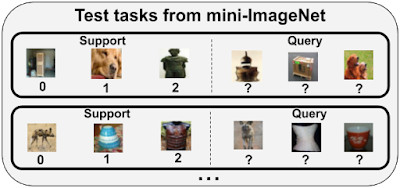
A popular dataset for studying few-shot classification is mini-ImageNet, a downsampled version of a subset of classes from ImageNet. This dataset contains 100 classes in total that are divided into training, validation and test class splits. While classes encountered at test time in benchmarks like mini-ImageNet have not been seen during training, they are still substantially similar to the training classes visually. Recent works reveal that this allows a model to perform competitively at test time simply by re-using features learned at training time, without necessarily demonstrating the capability to learn from the few examples presented to the model in the support set. In contrast, performing well on Meta-Dataset requires absorbing diverse information at training time and rapidly adapting it to solve significantly different tasks at test time that possibly originate from entirely unseen datasets.
Test tasks from mini-ImageNet. Each task is a classification problem between previously unseen (test) classes. The model can use the support set of a few labeled examples of the new classes to adapt to the task at hand and then predicts labels for the query examples of these new classes. The evaluation metric is the query set accuracy, averaged over examples within each task and across tasks.
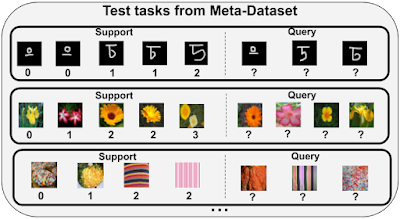
While other recent papers have investigated training on mini-ImageNet and evaluating on different datasets, Meta-Dataset represents the largest-scale organized benchmark for cross-dataset, few-shot image classification to date. It also introduces a sampling algorithm for generating tasks of varying characteristics and difficulty, by varying the number of classes in each task, the number of available examples per class, introducing class imbalances and, for some datasets, varying the degree of similarity between the classes of each task. Some example test tasks from Meta-Dataset are shown below.
Test tasks from Meta-Dataset. Contrary to the mini-ImageNet tasks shown above, different tasks here originate from (the test classes of) different datasets. Further, the number of classes and the support set sizes differ across tasks and the support sets might be class-imbalanced.
Initial Investigation and Findings on Meta-Dataset
We benchmark two main families of few-shot learning models on Meta-Dataset: pre-training and meta-learning.

Pre-training simply trains a classifier (a neural network feature extractor followed by a linear classifier) on the training set of classes using supervised learning. Then, the examples of a test task can be classified either by fine-tuning the pre-trained feature extractor and training a new task-specific linear classifier, or by means of nearest-neighbor comparisons, where the prediction for each query example is the label of its nearest support example. Despite its “baseline” status in the few-shot classification literature, this approach has recently enjoyed a surge of attention and competitive results.

On the other hand, meta-learners construct a number of “training tasks” and their training objective explicitly reflects the goal of performing well on each task’s query set after having adapted to that task using the associated support set, capturing the ability that is required at test time to solve each test task. Each training task is created by randomly sampling a subset of training classes and some examples of those classes to play the role of support and query sets.

Below, we summarize some of our findings from evaluating pre-training and meta-learning models on Meta Dataset:

1) Existing approaches have trouble leveraging heterogeneous training data sources.

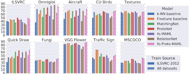
We compared training models (from both pre-training and meta-learning approaches) using only the training classes of ImageNet to using all training classes from the datasets in Meta-Dataset, in order to measure the generalization gain from using a more expansive collection of training data. We singled out ImageNet for this purpose, because the features learned on ImageNet readily transfer to other datasets. The evaluation tasks applied to all models are derived from a held-out set of classes from the datasets used in training, with at least two additional datasets that are entirely held-out for evaluation (i.e., no classes from these datasets were used for training).

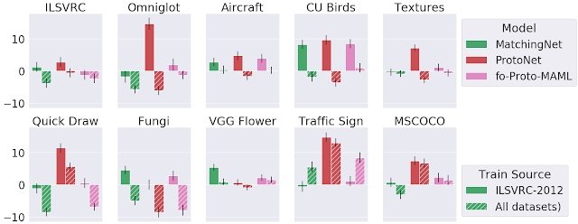
One might expect that training on more data, albeit heterogeneous, would generalize better on the test set. However, this is not always the case. Specifically, the following figure displays the accuracy of different models on test tasks of Meta-Dataset’s ten datasets. We observe that the performance on test tasks coming from handwritten characters / doodles (Omniglot and Quickdraw) is significantly improved when having trained on all datasets, instead of ImageNet only. This is reasonable since these datasets are visually significantly different from ImageNet. However, for test tasks of natural image datasets, similar accuracy can be obtained by training on ImageNet only, revealing that current models cannot effectively leverage heterogeneous data towards improving in this regard.
Comparison of test performance on each dataset after having trained on ImageNet (ILSVRC-2012) only or on all datasets.
2) Some models are more capable than others of exploiting additional data at test time.

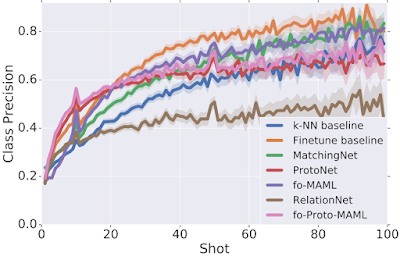
We analyzed the performance of different models as a function of the number of available examples in each test task, uncovering an interesting trade-off: different models perform best with a particular number of training (support) samples. We observe that some models outshine the rest when there are very few examples (“shots”) available (e.g., ProtoNet and our proposed fo-Proto-MAML) but don’t exhibit a large improvement when given more, while other models are not well-suited for tasks with very few examples but improve at a quicker rate as more are given (e.g., Finetune baseline). However, since in practice we might not know in advance the number of examples that will be available at test time, one would like to identify a model that can best leverage any number of examples, without disproportionately suffering in a particular regime.
Comparison of test performance averaged across different datasets to the number of examples available per class in test tasks (“shots”). Performance is measured in terms of class precision: the proportion of the examples of a class that are correctly labeled, averaged across classes.
3) The adaptation algorithm of a meta-learner is more heavily responsible for its performance than the fact that it is trained end-to-end (i.e. meta-trained).

We developed a new set of baselines to measure the benefit of meta-learning. Specifically, for several meta-learners, we consider a non-meta-learned counterpart that pre-trains a feature extractor and then, at evaluation time only, applies the same adaptation algorithm as the respective meta-learner on those features. When training on ImageNet only, meta-training often helps a bit or at least doesn’t hurt too much, but when training on all datasets, the results are mixed. This suggests that further work is needed to understand and improve upon meta-learning, especially across datasets.
Comparison of three different meta-learner variants to their corresponding inference-only baselines, when training on ImageNet (ILSVRC-1012) only or all datasets. Each bar represents the difference between meta-training and inference-only, so positive values indicate improved performance from meta-training.
Conclusion
Meta-Dataset introduces new challenges for few-shot classification. Our initial exploration has revealed limitations of existing methods, calling for additional research. Recent works have already reported exciting results on Meta-Dataset, for example using cleverly-designed task conditioning, more sophisticated hyperparameter tuning, a ‘meta-baseline’ that combines the benefits of pre-training and meta-learning, and finally using feature selection to specialize a universal representation for each task. We hope that Meta-Dataset will help drive research in this important sub-field of machine learning.

Acknowledgements
Meta-Dataset was developed by Eleni Triantafillou, Tyler Zhu, Vincent Dumoulin, Pascal Lamblin, Utku Evci, Kelvin Xu, Ross Goroshin, Carles Gelada, Kevin Swersky, Pierre-Antoine Manzagol and Hugo Larochelle. We would like to thank Pablo Castro for his valuable guidance on this blog post, Chelsea Finn for fruitful discussions and ensuring the correctness of fo-MAML’s implementation, as well as Zack Nado and Dan Moldovan for the initial dataset code that was adapted, Cristina Vasconcelos for spotting an issue in the ranking of models and John Bronskill for suggesting that we experiment with a larger inner-loop learning rate for MAML which indeed significantly improved our fo-MAML results.

Source: Google AI Blog


Applying Machine Learning to…..Yeast?


Humans have a long history with yeast, tied to the beginnings of plant domestication — baker’s (or brewer’s) yeast, Saccharomyces cerevisiae, has been used to make grains more digestible in the form of bread (or beer) for millennia. Today, yeast still has a large impact, with biologists adopting it as a model organism for biological research, genetics in particular, because it is easy to grow in the lab and is a eukaryote (i.e., unlike bacteria, it has a cell nucleus, like our cells do). It has even earned its own catchphrase in the biological community — “the awesome power of yeast genetics”. Studying the fundamentals of genetics is much easier in yeast, but is still applicable to humans since ~1000 yeast genes have a sequence homolog to human ones. Understanding how genes work together as a system is core to understanding all living things, which drives interest in this microorganism.

In collaboration with Calico Life Sciences, we present “Learning causal networks using inducible transcription factors and transcriptome-wide time series”, published in Molecular Systems Biology. Based on exhaustive experiments, we built a genome-wide model for the regulation of gene expression in S. cerevisiae and verified some of the results experimentally, enabling future investigations into less well understood biological systems. The Induction Dynamics gene Expression Atlas is available from Calico in a format easy to manipulate in python, with open-sourced code to do this on the Google Research GitHub. The data is hosted in a standard format at the Gene Expression Omnibus.

Using Yeast to Provide Insight into Aging
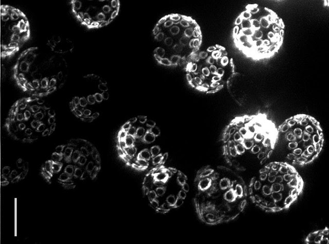
Yeast reproduce through a process called budding, in which a small bud grows from the surface of the parent to produce an offspring that is almost genetically identical. Interestingly, even though yeast are single-celled organisms, they grow old and die, typically after 30 budding events. In fact the “scars” from budding are clearly visible under a powerful microscope, allowing one to tell the age of the cell simply by looking! The problem is that researchers still do not know what causes aging to happen.
Bud scars on old yeast cells (5 μm bar for scale) — Photo Credit: Ian Foe, (Calico)
Scientists at Calico Life Sciences have pioneered a technique to make targeted perturbations to gene expression in yeast (i.e., allowing them to selectively “turn on” a gene’s activity) with the goal of understanding how aging works at the molecular level. The hope is that understanding aging in yeast will apply to aging in more complex organisms, like humans. This work is an early step in building a predictive framework for understanding the behavior of cells over time.

The Gene Expression Experiment
Genes encoded in DNA only function after being transcribed to RNA. It’s the RNA that is “translated” or “read” by ribosomes to produce protein. The level of protein production is governed by how much RNA is transcribed from DNA. Most of the work in a cell is being done by proteins, so they are key to understanding cell behavior. Yet, while we’d really like to measure the protein production levels, techniques to identify proteins at this scale are prohibitively expensive. Instead, in this experiment we use RNA as a proxy, since measuring RNA levels is easier.

The gene expression experiment is designed to perturb individual genes and measure, over time, how every other gene in the genome responds. The ability to rapidly perturb and track dynamics allows us to learn causal relationships and non-linear behaviors missing in most experiments. These dynamic data can also be used to train predictive models. This is made possible by strains of yeast with a single gene that is responsive to an external switch, in this case the hormone β-estradiol. To perturb a gene, the hormone is introduced, causing the switched gene to be overexpressed by a factor of 50 within 10 minutes. The yeast culture is then sampled at several points in time to measure the gene expression levels on microarrays. These experiments were done in parallel, with one yeast strain per culture, running concurrently.

Most of the perturbation experiments were done on a particular class of genes coding for transcription factors (TFs). These genes are the primary regulators of gene expression, coding for proteins that actually bind to the DNA strands, permitting or blocking transcription of particular genes.

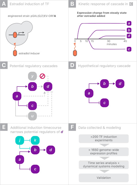
When gene “a” is turned on it may upregulate gene “b” and downregulate gene “c”, and later lead to upregulation of gene “d”. Since yeast has more than 6000 genes, tracing the downstream impact of perturbing a single gene can get complicated very quickly. By combining experiments on different genes, one hopes to disambiguate the exact regulation mechanisms.
Schematic of the genome perturbation experiment: yeast strain with switchable gene “a”. Turning on a single gene (A) can result in differing levels of gene expression over time (B). Tracking these changes in comparison to those induced by turning on other genes (C and D) can provide insight into the regulation mechanisms (E).
The Gene Expression Model
For this experiment, we partnered with Calico because of the scale of the data, and the opportunity to leverage Google’s machine learning expertise and compute resources. There were more than 200 perturbation experiments on different yeast strains, each activating a single gene. In each experiment, the expression levels of all 6000 genes were measured eight times over 90 minutes, yielding a total of almost 20 million individual measurements (panel F, above). Clearly some automation was required to analyze the data.

Our approach was to model the whole process as a system of differential equations: the rate of change of the expression of a gene was proportional to a weighted sum of the expression levels of all genes. We first estimated the time derivatives from the data by simply subtracting the expression levels among adjacent time points. We then predicted the time derivatives using only the raw expression levels themselves. By fitting a linear regression, we are, in effect, fitting the coefficients of a system of differential equations describing gene regulation. Our hope is that the differential equation model would be a low dimensional representation of the data that could be interpreted more easily. To handle overfitting, we regularized the model using the L1-norm, which prefers to set uninformative parameters to exactly zero.

Because each of the 200 experiments was unique, we held out each one in turn, refitting the model and allowing the selection of the best hyperparameters to optimize the out-of-sample loss. In the end, the work required a significant amount of compute, amounting to more than 50 million full regularization paths.

Model Results
Our model made predictions about which genes would code for intermediate regulators of gene expression. This is an attempt at modeling the full gene regulation network of the organism. To verify these predictions, our collaborators at Calico collected more data from ten new strains of yeast. Three out of ten of the predictions held up in these experiments. One of the genes that the model predicted to be active encoded an unverified transcription factor, while another previously identified as a regulator but never followed up, was found by our model to be a very active regulator. Our model was able to identify these without prior biological knowledge, demonstrating that these ML techniques might scale to other domains or organisms that are much less well studied.

More discussion of the impact of this work within the broad context of the field of genomics is available in an independent peer commentary.

Acknowledgements
We wish to thank Marc Coram, Minjie Fan, and Marc Berndl for their foundational contributions to this work, the Google Accelerated Science team for their continual support, and the entire team at Calico for the opportunity to collaborate on this experiment.

Source: Google AI Blog


Yet More Google Compute Cluster Trace Data


Google’s Borg cluster management system supports our computational fleet, and underpins almost every Google service. For example, the machines that host the Google Doc used for drafting this post are managed by Borg, as are those that run Google’s cloud computing products. That makes the Borg system, as well as its workload, of great interest to researchers and practitioners.

Eight years ago Google published a 29-day cluster trace — a record of every job submission, scheduling decision, and resource usage data for all the jobs in a Google Borg compute cluster, from May 2011. That trace has enabled a wide range of research on advancing the state of the art for cluster schedulers and cloud computing, and has been used to generate hundreds of analyses and studies. But in the years since the 2011 trace was made available, machines and software have evolved, workloads have changed, and the importance of workload variance has become even clearer.

To help researchers explore these changes themselves, we have released a new trace dataset for the month of May 2019 covering eight Google compute clusters. This new dataset is both larger and more extensive than the 2011 one, and now includes:
  • CPU usage information histograms for each 5 minute period, not just a point sample;
  • information about alloc sets (shared resource reservations used by jobs);
  • job-parent information for master/worker relationships such as MapReduce jobs.
Just like the last trace, the new one focuses on resource requests and usage, and contains no information about end users, their data, or patterns of access to storage systems and other services.

At this time, we are making the trace data available via Google BigQuery so that sophisticated analyses can be performed without requiring local resources. This site provides access instructions and a detailed description of what the traces contain.

A first analysis of differences between the 2011 and 2019 traces appears in this paper.

We hope this data will facilitate even more research into cluster management. Do let us know if you find it useful, publish papers that use it, develop tools that analyze it, or have suggestions for how to improve it.

Acknowledgements
I’d especially like to thank our intern Muhammad Tirmazi, and my colleagues Nan Deng, Md Ehtesam Haque, Zhijing Gene Qin, Steve Hand and Visiting Researcher Adam Barker for doing the heavy lifting of preparing the new trace set.

Source: Google AI Blog


Open Images V6 — Now Featuring Localized Narratives


Open Images is the largest annotated image dataset in many regards, for use in training the latest deep convolutional neural networks for computer vision tasks. With the introduction of version 5 last May, the Open Images dataset includes 9M images annotated with 36M image-level labels, 15.8M bounding boxes, 2.8M instance segmentations, and 391k visual relationships. Along with the dataset itself, the associated Open Images Challenges have spurred the latest advances in object detection, instance segmentation, and visual relationship detection.
Annotation modalities in Open Images V5: image-level labels, bounding boxes, instance segmentations, and visual relationships. Image sources: 1969 Camaro RS/SS by D. Miller, the house by anita kluska, Cat Cafe Shinjuku calico by Ari Helminen, and Radiofiera - Villa Cordellina Lombardi, Montecchio Maggiore (VI) - agosto 2010 by Andrea Sartorati. All images used under CC BY 2.0 license.
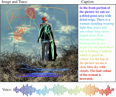
Today, we are happy to announce the release of Open Images V6, which greatly expands the annotation of the Open Images dataset with a large set of new visual relationships (e.g., “dog catching a flying disk”), human action annotations (e.g., “woman jumping”), and image-level labels (e.g., “paisley”). Notably, this release also adds localized narratives, a completely new form of multimodal annotations that consist of synchronized voice, text, and mouse traces over the objects being described. In Open Images V6, these localized narratives are available for 500k of its images. Additionally, in order to facilitate comparison to previous works, we also release localized narratives annotations for the full 123k images of the COCO dataset.
Sample of localized narratives. Image source: Spring is here:-) by Kasia.
Localized Narratives
One of the motivations behind localized narratives is to study and leverage the connection between vision and language, typically done via image captioning — images paired with human-authored textual descriptions of their content. One of the limitations of image captioning, however, is the lack of visual grounding, that is, localization on the image of the words in the textual description. To mitigate that, some previous works have a-posteriori drawn the bounding boxes for the nouns present in the description. In contrast, in localized narratives, every word in the textual description is grounded.
Different levels of grounding between image content and captioning. Left to Right: Caption to whole image (COCO); nouns to boxes (Flickr30k Entities); each word to a mouse trace segment (localized narratives). Image sources: COCO, Flickr30k Entities, and Sapa, Vietnam by Rama.
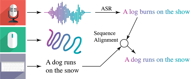
Localized narratives are generated by annotators who provide spoken descriptions of an image while they simultaneously move their mouse to hover over the regions they are describing. Voice annotation is at the core of our approach since it directly connects the description with the regions of the image it is referencing. To make the descriptions more accessible, the annotators manually transcribed their description, which was then aligned with the automatic speech transcription result. This recovers the timestamps for the description, ensuring that the three modalities (speech, text, and mouse trace) are correct and synchronized.
Alignment of manual and automatic transcriptions. Icons based on an original design from Freepik.
Speaking and pointing simultaneously are very intuitive, which allowed us to give the annotators very vague instructions about the task. This creates potential avenues of research for studying how people describe images. For example, we observed different styles when indicating the spatial extent of an object — circling, scratching, underlining, etc. — the study of which could bring valuable insights for the design of new user interfaces.
Mouse trace segments corresponding to the words below the images. Image sources: Via Guglielmo Marconi, Positano - Hotel Le Agavi - boat by Elliott Brown, air frame by vivek jena, and CL P1050512 by Virginia State Parks.
To get a sense of the amount of additional data these localized narratives represent, the total length of mouse traces is ~6400 km long, and if read aloud without stopping, all the narratives would take ~1.5 years to listen to!

New Visual Relationships, Human Actions, and Image-Level Annotations
In addition to the localized narratives, in Open Images V6 we increased the types of visual relationship annotations by an order of magnitude (up to 1.4k), adding for example “man riding a skateboard”, “man and woman holding hands”, and “dog catching a flying disk”.
Image sources: IMG_5678.jpg by James Buck, DSC_0494 by Quentin Meulepas, and DSC06464 by sally9258.
People in images have been at the core of computer vision interests since its inception and understanding what those people are doing is of utmost importance for many applications. That is why Open Images V6 also includes 2.5M annotations of humans performing standalone actions, such as “jumping”, “smiling”, or “laying down”.
Image sources: _DSCs1341 (2) by Boo Ph, and Richard Wagner Spiele 2015 by Johannes Gärtner.
Finally, we also added 23.5M new human-verified image-level labels, reaching a total of 59.9M over nearly 20,000 categories.

Conclusion
Open Images V6 is a significant qualitative and quantitative step towards improving the unified annotations for image classification, object detection, visual relationship detection, and instance segmentation, and takes a novel approach in connecting vision and language with localized narratives. We hope that Open Images V6 will further stimulate progress towards genuine scene understanding.

Source: Google AI Blog


Enhancing the Research Community’s Access to Street View Panoramas for Language Grounding Tasks


Significant advances continue to be made in both natural language processing and computer vision, but the research community is still far from having computer agents that can interpret instructions in a real-world visual context and take appropriate actions based on those instructions. Agents, including robots, can learn to navigate new environments, but they cannot yet understand instructions such as, “Go forward and turn left after the red fire hydrant by the train tracks. Then go three blocks and stop in front of the building with a row of flags over its entrance.” Doing so requires relating verbal descriptions like train tracks, red fire hydrant, and row of flags to their visual appearance, understanding what a block is and how to count three of them, relating objects based on spatial configurations such as by and over, relating directions such as go forward and turn left to actions, and much more.

Grounded language understanding problems of this form are excellent testbeds for research on computational intelligence in that they are easy for people but hard for current agents, they synthesize language, perception and action, and evaluation of successful completion is straightforward. Progress on such problems can greatly enhance the ability of agents to coordinate movement and action with people. However finding or creating datasets large and diverse enough for developing robust models is difficult.

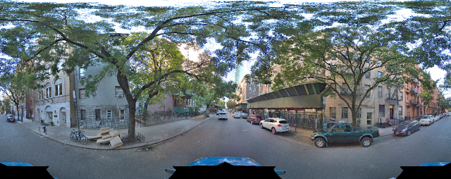
An ideal resource for quickly training and evaluating agents on grounded language understanding tasks is Street View imagery, an extensive and visually rich virtual representation of the world. Street View is integrated with Google Maps and is composed of billions of street-level panoramas. The Touchdown dataset, created by researchers at Cornell Tech, represents a compelling example of using Street View to drive research on grounded language understanding. However, due to restrictions on access to Street View panoramas, Touchdown can only provide panorama IDs rather than the panoramas themselves, sometimes making it difficult for the broader research community to work on Touchdown’s tasks: vision-and-language navigation (VLN), in which instructions are presented for navigation through streets, and spatial description resolution (SDR), which requires resolving spatial descriptions from a given viewpoint.

In “Retouchdown: Adding Touchdown to StreetLearn as a Shareable Resource for Language Grounding Tasks in Street View,” we address this problem by adding the Street View panoramas referenced in the Touchdown tasks to the existing StreetLearn dataset. Using this data, we generate a model that is fully compatible with the tasks defined in Touchdown. Additionally, we have provided open source TensorFlow implementations for the Touchdown tasks as part of the VALAN toolkit.

Grounded Language Understanding Tasks
Touchdown’s two grounded language understanding tasks can be used as benchmarks for navigation models. VLN involves following instructions from one street location to another, while SDR requires identifying a point in a Street View panorama given a description based on its surrounding visual context. The two tasks are shown being performed together in the animation below.
Example animation of a person following Touchdown instructions: “Orient yourself so that the umbrellas are to the right. Go straight and take a right at the first intersection. At the next intersection there should be an old-fashioned store to the left. There is also a dinosaur mural to the right. Touchdown is on the back of the dinosaur.”
Touchdown’s VLN task is similar to that defined in the popular Room-to-Room dataset, except that Street View has far greater visual diversity and more degrees of freedom for movement. Performance of the baseline models in Touchdown leaves considerable headroom for innovation and improvement on many facets of the task, including linguistic and visual representations, their integration, and learning to take actions conditioned on them.

That said, while enabling the broader research community to work with Touchdown’s tasks, certain safeguards are needed to make it compliant with the Google Maps/Google Earth Terms of Service and protect the needs of both Google and individuals. For example, panoramas may not be mass downloaded, nor can they be stored indefinitely (for example, individuals may ask to remove specific panoramas). Therefore, researchers must periodically delete and refresh panoramas in order to work with the data while remaining compliant with these terms.

StreetLearn: A Dataset of Approved Panoramas for Research Use
An alternative way to interact with Street View panoramas was forged by DeepMind with the StreetLearn data release last year. With StreetLearn, interested researchers can fill out a form requesting access to a set of 114k panoramas for regions of New York City and Pittsburgh. Recently, StreetLearn has been used to support the StreetNav task suite, which includes training and evaluating agents that follow Google Maps directions. This is a VLN task like Touchdown and Room-to-Room; however, it differs greatly in that it does not use natural language provided by people.

Additionally, even though StreetLearn’s panoramas cover the same area of Manhattan as Touchdown, they are not adequate for research covering the tasks defined in Touchdown, because those tasks require the exact panoramas that were used during the Touchdown annotation process. For example, in Touchdown tasks, the language instructions refer to transient objects such as cars, bicycles, and couches. A Street View panorama from a different time period may not contain these objects, so the instructions are not stable across time periods.
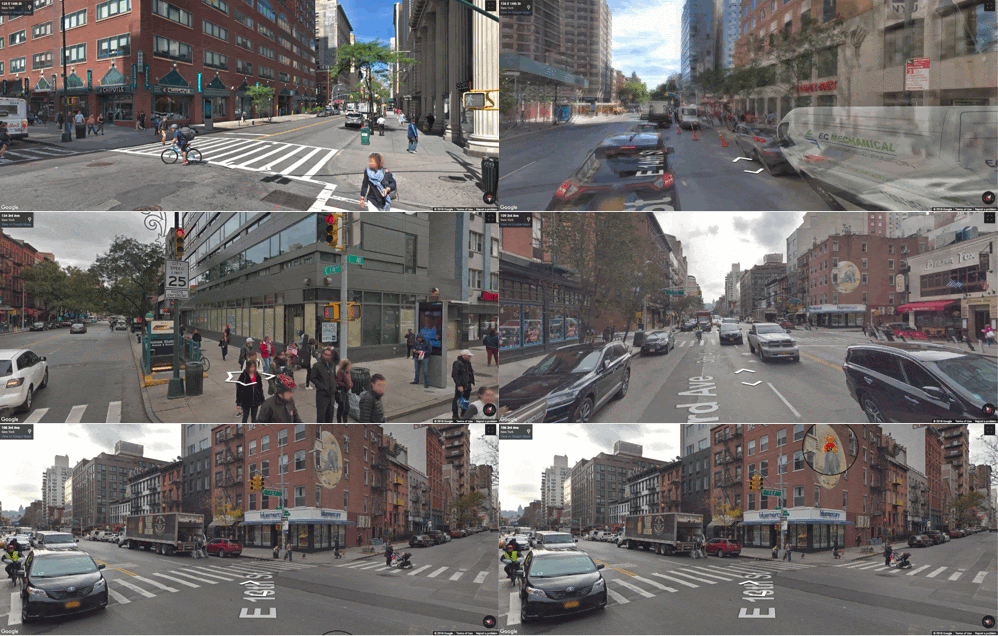
Touchdown instruction: “Two parked bicycles, and a discarded couch, all on the left. Walk just past this couch, and stop before you pass another parked bicycle. This bike will be white and red, with a white seat. Touchdown is sitting on top of the bike seat.” Other panoramas from the same location taken at other times would be highly unlikely to contain these exact items in the exact same positions. For a concrete example, see the current imagery available for this location in Street View, which contains very different transient objects.
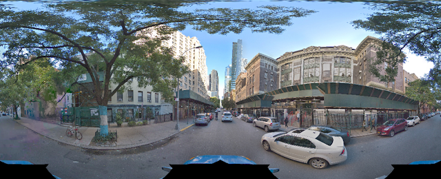
Furthermore, SDR requires coverage of multiple points-of-view for those specific panoramas. For example, the following panorama is one step down the street from the previous one. They may look similar, but they are in fact quite different — note that the bikes seen on the left side in both panoramas are not  the same — and the location of Touchdown is toward the middle of the above panorama (on the bike seat) and to the bottom left in the second panorama. As such, the pixel location of the SDR problem is different for different panoramas, but consistent with respect to the real world location referred to in the instruction. This is especially important for the end-to-end task of following both the VLN and SDR instructions together: if an agent stops, they should be able to complete the SDR task regardless of their exact location (provided the target is visible).
A panorama one step farther down the street from the previous scene.
Another problem is that the granularity of the panorama spacing is different. The figure below shows the overlap between the StreetLearn (blue) and Touchdown (red) panoramas in Manhattan. There are 710 panoramas (out of 29,641) that share the same ID in both datasets (in black). Touchdown covers half of Manhattan and the density of the panoramas is similar, but the exact locations of the nodes visited differ.
Adding Touchdown Panoramas to StreetLearn and Verifying Model Baselines
Retouchdown reconciles Touchdown’s mode of dissemination with StreetLearn’s, which was originally designed to adhere to the rights of Google and individuals while also simplifying access to researchers and improving reproducibility. Retouchdown includes both data and code that allows the broader research community to work effectively with the Touchdown tasks — most importantly to ensure access to the data and to ease reproducibility. To this end, we have integrated the Touchdown panoramas into the StreetLearn dataset to create a new version of StreetLearn with 144k panoramas (an increase of 26%) that are all approved for research use.

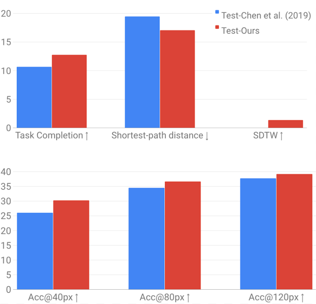
We also reimplemented models for VLN and SDR and show that they are on par or better than the results obtained in the original Touchdown paper. These implementations are open-sourced as well, as part of the VALAN toolkit. The first graph below compares the results of Chen et al. (2019) to our reimplementation for the VLN task. It includes the SDTW metric, which measures both successful completion and fidelity to the true reference path. The second graph below makes the same comparison for the SDR task. For SDR, we show accuracy@npx measurements, which provides the percent of times the model’s prediction is within n pixels of the goal location in the image. Our results are slightly better due to some small differences in models and processing, but most importantly, the results show that the updated panoramas are fully capable of supporting future modeling for the Touchdown tasks.
Performance comparison between Chen et al. (2019) using the original panoramas (in blue) and our reimplementation using the panoramas available in StreetLearn (in red). Top: VLN results for task completion, shortest path distance and success weighted by Dynamic Time Warping (SDTW). Bottom: SDR results for the accuracy@npx metrics.
Obtaining the Data
Researchers interested in working with the panoramas should fill out the StreetLearn interest form. Subject to approval, they will be provided with a download link. Their information is held so that the StreetLearn team can inform them of updates to the data. This allows both Google and participating researchers to effectively and easily respect takedown requests. The instructions and panorama connectivity data can be obtained from the Touchdown github repository.

It is our hope that this release of these additional panoramas will enable the research community to make further progress on these challenging grounded language understanding tasks.

Acknowledgements
The core team includes Yoav Artzi, Eugene Ie, and Piotr Mirowski. We would like to thank Howard Chen for his help with reproducing the Touchdown results, Larry Lansing, Valts Blukis and Vihan Jain for their help with the code and open-sourcing, and the Language team in Google Research, especially Radu Soricut, for the insightful comments that contributed to this work. Many thanks also to the Google Maps and Google Street View teams for their support in accessing and releasing the data, and to the Data Compute team for reviewing the panoramas.

Source: Google AI Blog


TyDi QA: A Multilingual Question Answering Benchmark


Question answering technologies help people on a daily basis — when faced with a question, such as “Is squid ink safe to eat?”, users can ask a voice assistant or type a search and expect to receive an answer. Last year, we released the English-language Natural Questions dataset to the research community to provide a challenge that reflects the needs of real users. However, there are thousands of different languages, and many of those use very different approaches to construct meaning. For example, while English changes words to indicate one object (“book”) versus many (“books”), Arabic also has a third form to indicate if there are two of something ("كتابان", kitaban) beyond just singular ("كتاب", kitab) or plural ("كتب", kutub). In addition, some languages, such as Japanese, do not use spaces between words. Creating machine learning systems that can understand the many ways languages express meaning is challenging, and training such systems requires examples from the diverse the languages to which they will be applied.

To encourage research on multilingual question-answering, today we are releasing TyDi QA, a question answering corpus covering 11 Typologically Diverse languages. Described in our paper, “TyDi QA: A Benchmark for Information-Seeking Question Answering in Typologically Diverse Languages”, our corpus is inspired by typological diversity, a notion that different languages express meaning in structurally different ways. Because we selected a set of languages that are typologically distant from each other for this corpus, we expect models performing well on this dataset to generalize across a large number of the languages in the world.

A Typologically Diverse Collection of Languages
TyDi QA includes over 200,000 question-answer pairs from 11 languages representing a diverse range of linguistic phenomena and data challenges. Many of these languages use non-Latin alphabets, such as Arabic, Bengali, Korean, Russian, Telugu, and Thai. Others form words in complex ways, including Arabic, Finnish, Indonesian, Kiswahili, Russian. Japanese uses four alphabets (shown by the four colors in “24時間でのサーキット周回数”) while the Korean alphabet itself is highly compositional. These languages also range from having much available data on the web (English and Arabic) to very little (Bengali and Kiswahili). We expect that systems that can address these challenges will be successful for a very large number of languages.

Creating Realistic Data
Many early QA datasets used by the research community were created by first showing paragraphs to people and then asking them to write questions based on what could be answered from reading the paragraph. However, since people could see the answer while writing each question, this approach yielded questions that often contained the same words as the answer. As a result, machine learning algorithms trained on such data would favor word matching, oblivious to the more nuanced answers required to satisfy users’ needs.

To construct a more natural dataset, we collected questions from people who wanted an answer, but did not know the answer yet. To inspire questions, we showed people an interesting passage from Wikipedia written in their native language. We then had them ask a question, any question, as long as it was not answered by the passage and they actually wanted to know the answer. This is similar to how your own curiosity might spawn questions about interesting things you see while walking down the street. We encouraged our question writers to let their imaginations run. Does a passage about ice make you think about popsicles in summer? Great! Ask who invented popsicles. Importantly, questions were written directly in each language, not translated, so many questions are unlike those seen in an English-first corpus. One question in Bengali asks, “সফেদা ফল খেতে কেমন?” (What does sapodilla taste like?) Never heard of it? That’s probably because it’s grown much more commonly in India than the U.S.

For each of these questions, we performed a Google Search for the best-matching Wikipedia article in the appropriate language and asked a person to find and highlight the answer within that article. While we expected some interesting divergences between the question and answers when the question writers did not have the answers in front of them, combined with the astonishing breadth of linguistic phenomena in the world’s languages, we found that the situation was even more complex.

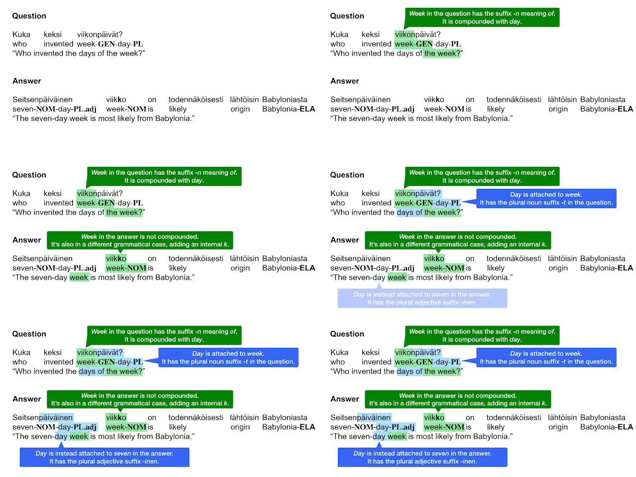
For example, in Finnish, there are fascinating examples in which the words day and week are represented very differently in the question and answer. To be successful in selecting this answer sentence out of an entire Wikipedia article, a system needs to be able to recognize the relationship among the Finnish words viikonpäivät, seitsenpäiväinen, and viikko

Making Progress Together as a Research Community
It is our hope that this dataset will push the research community to innovate in ways that will create more helpful question-answering systems for users around the world. To track the community’s progress, we have established a leaderboard where participants can evaluate the quality of their machine learning systems and are also open-sourcing a question answering system that uses the data. Please visit the challenge website to view the leaderboard and learn more.

Acknowledgements
This dataset is the result of a team of many Googlers including (alphabetically) Dan Garrette, Eunsol Choi, Jennimaria Palomaki, Michael Collins, Tom Kwiatkowski, and Vitaly Nikolaev. The Finnish gloss above is by Jennimaria Palomaki.

Source: Google AI Blog