Tag Archives: Computer Vision

Lidar-Camera Deep Fusion for Multi-Modal 3D Detection

LiDAR and visual cameras are two types of complementary sensors used for 3D object detection in autonomous vehicles and robots. LiDAR, which is a remote sensing technique that uses light in the form of a pulsed laser to measure ranges, provides low-resolution shape and depth information, while cameras provide high-resolution shape and texture information. While the features captured by LiDAR and cameras should be merged together to provide optimal 3D object detection, it turns out that most state-of-the-art 3D object detectors use LiDAR as the only input. The main reason is that to develop robust 3D object detection models, most methods need to augment and transform the data from both modalities, making the accurate alignment of the features challenging.

Existing algorithms for fusing LiDAR and camera outputs, such as PointPainting, PointAugmenting, EPNet, 4D-Net and ContinuousFusion, generally follow two approaches — input-level fusion where the features are fused at an early stage, decorating points in the LiDAR point cloud with the corresponding camera features, or mid-level fusion where features are extracted from both sensors and then combined. Despite realizing the importance of effective alignment, these methods struggle to efficiently process the common scenario where features are enhanced and aggregated before fusion. This indicates that effectively fusing the signals from both sensors might not be straightforward and remains challenging.

In our CVPR 2022 paper, “DeepFusion: LiDAR-Camera Deep Fusion for Multi-Modal 3D Object Detection”, we introduce a fully end-to-end multi-modal 3D detection framework called DeepFusion that applies a simple yet effective deep-level feature fusion strategy to unify the signals from the two sensing modalities. Unlike conventional approaches that decorate raw LiDAR point clouds with manually selected camera features, our method fuses the deep camera and deep LiDAR features in an end-to-end framework. We begin by describing two novel techniques, InverseAug and LearnableAlign, that improve the quality of feature alignment and are applied to the development of DeepFusion. We then demonstrate state-of-the-art performance by DeepFusion on the Waymo Open Dataset, one of the largest datasets for automotive 3D object detection.

InverseAug: Accurate Alignment under Geometric Augmentation
To achieve good performance on existing 3D object detection benchmarks for autonomous cars, most methods require strong data augmentation during training to avoid overfitting. However, the necessity of data augmentation poses a non-trivial challenge in the DeepFusion pipeline. Specifically, the data from the two modalities use different augmentation strategies, e.g., rotating along the z-axis for 3D point clouds combined with random flipping for 2D camera images, often resulting in alignment that is inaccurate. Then the augmented LiDAR data has to go through a voxelization step that converts the point clouds into volume data stored in a three dimensional array of voxels. The voxelized features are quite different compared to the raw data, making the alignment even more difficult. To address the alignment issue caused by geometry-related data augmentation, we introduce Inverse Augmentation (InverseAug), a technique used to reverse the augmentation before fusion during the model’s training phase.

In the example below, we demonstrate the difficulties in aligning the augmented LiDAR data with the camera data. In this case, the LiDAR point cloud is augmented by rotation with the result that a given 3D key point, which could be any 3D coordinate, such as a LiDAR data point, cannot be easily aligned in 2D space simply through use of the original LiDAR and camera parameters. To make the localization feasible, InverseAug first stores the augmentation parameters before applying the geometry-related data augmentation. At the fusion stage, it reverses all data augmentation to get the original coordinate for the 3D key point, and then finds its corresponding 2D coordinates in the camera space.

During training, InverseAug resolves the inaccurate alignment from geometric augmentation.
Left: Alignment without InverseAug. Right: Alignment quality improvement with InverseAug.

LearnableAlign: A Cross-Modality-Attention Module to Learn Alignment
We also introduce Learnable Alignment (LearnableAlign), a cross-modality-attention–based feature-level alignment technique, to improve the alignment quality. For input-level fusion methods, such as PointPainting and PointAugmenting, given a 3D LiDAR point, only the corresponding camera pixel can be exactly located as there is a one-to-one mapping. In contrast, when fusing deep features in the DeepFusion pipeline, each LiDAR feature represents a voxel containing a subset of points, and hence, its corresponding camera pixels are in a polygon. So the alignment becomes the problem of learning the mapping between a voxel cell and a set of pixels.

A naïve approach is to average over all pixels corresponding to the given voxel. However, intuitively, and as supported by our visualized results, these pixels are not equally important because the information from the LiDAR deep feature unequally aligns with every camera pixel. For example, some pixels may contain critical information for detection (e.g., the target object), while others may be less informative (e.g., consisting of backgrounds such as roads, plants, occluders, etc.).

LearnableAlign leverages a cross-modality attention mechanism to dynamically capture the correlations between two modalities. Here, the input contains the LiDAR features in a voxel cell, and all its corresponding camera features. The output of the attention is essentially a weighted sum of the camera features, where the weights are collectively determined by a function of the LiDAR and camera features. More specifically, LearnableAlign uses three fully-connected layers to respectively transform the LiDAR features to a vector (ql), and camera features to vectors (kc) and (vc). For each vector (ql), we compute the dot products between (ql) and (kc) to obtain the attention affinity matrix that contains correlations between the LiDAR features and the corresponding camera features. Normalized by a softmax operator, the attention affinity matrix is then used to calculate weights and aggregate the vectors (vc) that contain camera information. The aggregated camera information is then processed by a fully-connected layer, and concatenated (Concat) with the original LiDAR feature. The output is then fed into any standard 3D detection framework, such as PointPillars or CenterPoint for model training.
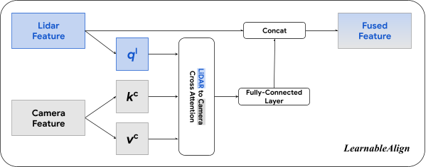
LearnableAlign leverages the cross-attention mechanism to align LiDAR and camera features.

DeepFusion: A Better Way to Fuse Information from Different Modalities
Powered by our two novel feature alignment techniques, we develop DeepFusion, a fully end-to-end multi-modal 3D detection framework. In the DeepFusion pipeline, the LiDAR points are first fed into an existing feature extractor (e.g., pillar feature net from PointPillars) to obtain LiDAR features (e.g., pseudo-images). In the meantime, the camera images are fed into a 2D image feature extractor (e.g., ResNet) to obtain camera features. Then, InverseAug and LearnableAlign are applied in order to fuse the camera and LiDAR features together. Finally, the fused features are processed by the remaining components of the selected 3D detection model (e.g., the backbone and detection head from PointPillars) to obtain the detection results.

The pipeline of DeepFusion.

Benchmark Results
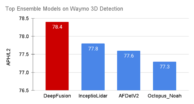
We evaluate DeepFusion on the Waymo Open Dataset, one of the largest 3D detection challenges for autonomous cars, using the Average Precision with Heading (APH) metric under difficulty level 2, the default metric to rank a model’s performance on the leaderboard. Among the 70 participating teams all over the world, the DeepFusion single and ensemble models achieve state-of-the-art performance in their corresponding categories.
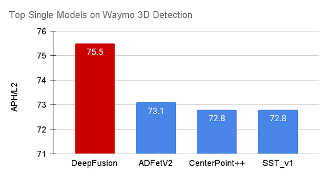
The single DeepFusion model achieves new state-of-the-art performance on Waymo Open Dataset.
The Ensemble DeepFusion model outperforms all other methods on Waymo Open Dataset, ranking No. 1 on the leaderboard.

The Impact of InverseAug and LearnableAlign
We also conduct ablation studies on the effectiveness of the proposed InverseAug and LearnableAlign techniques. We demonstrate that both InverseAug and LearnableAlign individually contribute to a performance gain over the LiDAR-only model, and combining both can further yield an even more significant boost.

Ablation studies on InverseAug (IA) and LearnableAlign (LA) measured in average precision (AP) and APH. Combining both techniques contributes to the best performance gain.

Conclusion
We demonstrate that late-stage deep feature fusion can be more effective when features are aligned well, but aligning features from two different modalities can be challenging. To address this challenge, we propose two techniques, InverseAug and LearnableAlign, to improve the quality of alignment among multimodal features. By integrating these techniques into the fusion stage of our proposed DeepFusion method, we achieve state-of-the-art performance on the Waymo Open Dataset.

Acknowledgements:
Special thanks to co-authors Tianjian Meng, Ben Caine, Jiquan Ngiam, Daiyi Peng, Junyang Shen, Bo Wu, Yifeng Lu, Denny Zhou, Quoc Le, Alan Yuille, Mingxing Tan.
Source: Google AI Blog


Learning from Weakly-Labeled Videos via Sub-Concepts

Video recognition is a core task in computer vision with applications from video content analysis to action recognition. However, training models for video recognition often requires untrimmed videos to be manually annotated, which can be prohibitively time consuming. In order to reduce the effort of collecting videos with annotations, learning visual knowledge from videos with weak labels, i.e., where the annotation is auto-generated without manual intervention, has attracted growing research interest, thanks to the large volume of easily accessible video data. Untrimmed videos, for example, are often acquired by querying with keywords for classes that the video recognition model aims to classify. A keyword, which we refer to as a weak label, is then assigned to each untrimmed video obtained.

Although large-scale videos with weak labels are easier to collect, training with unverified weak labels poses another challenge in developing robust models. Recent studies have demonstrated that, in addition to the label noise (e.g., incorrect action labels on untrimmed videos), there is temporal noise due to the lack of accurate temporal action localization — i.e., an untrimmed video may include other non-targeted content or may only show the target action in a small proportion of the video.

Reducing noise effects for large-scale weakly-supervised pre-training is critical but particularly challenging in practice. Recent work indicates that querying short videos (e.g., ~1 minute in length) to obtain more accurate temporal localization of target actions or applying a teacher model to do filtering can yield improved results. However, such data pre-processing methods prevent models from fully utilizing available video data, especially longer videos with richer content.

In "Learning from Weakly-Labeled Web Videos via Exploring Sub-Concepts", we propose a solution to these issues that uses a simple learning framework to conduct effective pre-training on untrimmed videos. Instead of simply filtering the potential temporal noise, this approach converts such “noisy” data to useful supervision by creating a new set of meaningful “middle ground” pseudo-labels that expand the original weak label space, a novel concept we call Sub-Pseudo Label (SPL). The model is pre-trained on this more "fine-grained" space and then fine-tuned on a target dataset. Our experiments demonstrate that the learned representations are much better than previous approaches. Moreover, SPL has been shown to be effective in improving the action recognition model quality for Google Cloud Video AI, which enables content producers to easily search through massive libraries of their video assets to quickly source content of interest.

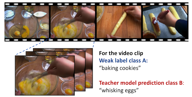
Sampled training clips may represent a different visual action (whisking eggs) from the query label of the whole untrimmed video (baking cookies). SPL converts the potential label noise to useful supervision signals by creating a new set of “middle ground” pseudo-classes (i.e., sub-concepts) via extrapolating two related action classes. Enriched supervision is provided for effective model pre-training.

Sub-Pseudo Label (SPL)
SPL is a simple technique that advances the teacher-student training framework, which is known to be effective for self-training and to improve semi-supervised learning. In the teacher-student framework, a teacher model is trained on high-quality labeled data and then assigns pseudo-labels to unlabeled data. The student model trains on both high-quality labeled data and the unlabeled data that has the teacher-predicted labels. While previous methods have proposed a number of ways to improve the pseudo-label quality, SPL takes a novel approach that combines knowledge from both weak labels (i.e., query text used to acquire data) and teacher-predicted labels, which results in better pseudo-labels overall. This method focuses on video recognition where temporal noise is challenging, but it can be extended easily to other domains, like image classification.

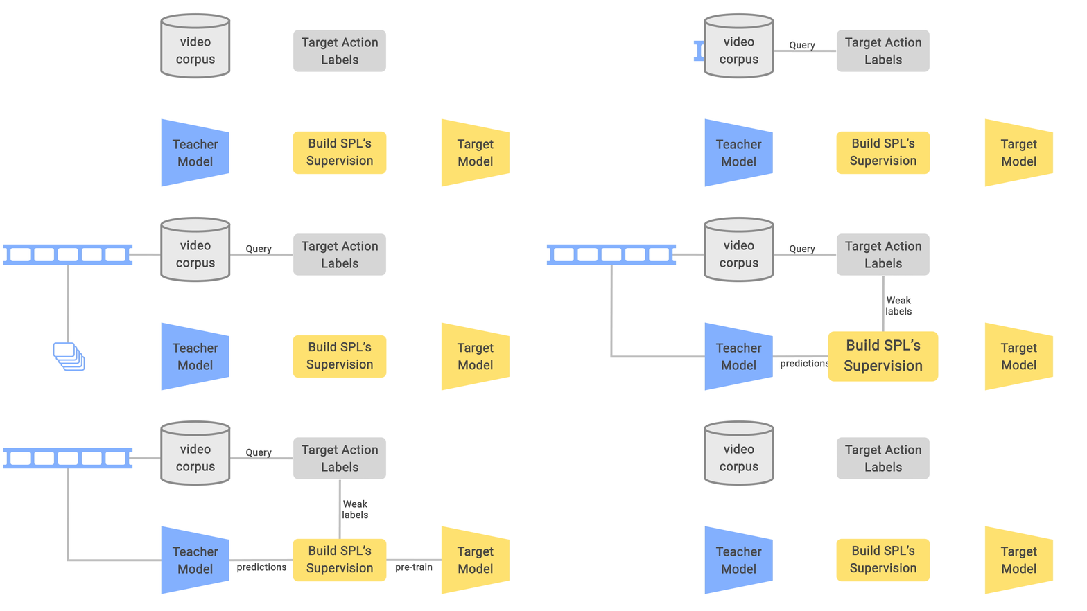
The overall pre-training framework for learning from weakly labeled videos via SPLs. Each trimmed video clip is re-labeled using SPL given the teacher-predicted labels and the weak labels used to query the corresponding untrimmed video.

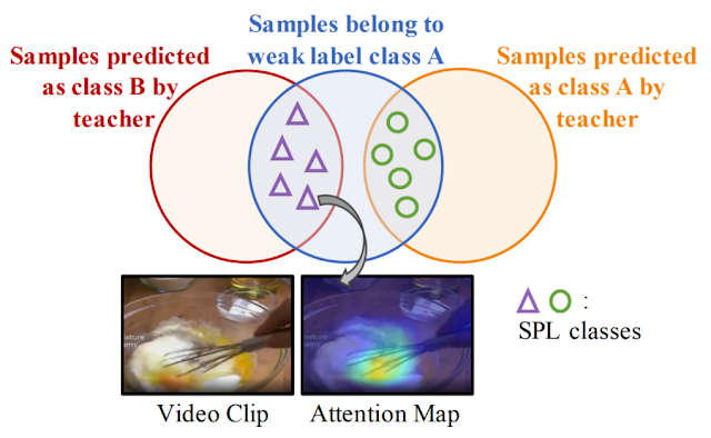
The SPL method is motivated by the observation that within an untrimmed video “noisy” video clips have semantic relations with the target action (i.e., the weak label class), but may also include essential visual components of other actions, such as the teacher model–predicted class. Our approach uses the extrapolated SPLs from weak labels together with the distilled labels to capture the enriched supervision signals, encouraging learning better representations during pre-training that can be used for downstream fine-tuning tasks.

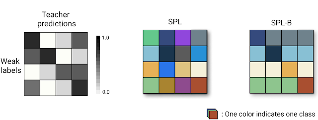
It is straightforward to determine the SPL class for each video clip. We first perform inference on each video clip using the teacher model trained from a target dataset to get a teacher prediction class. Each clip is also labeled by the class (i.e., query text) of the untrimmed source video. A 2-dimensional confusion matrix is used to summarize the alignments between the teacher model inferences and the original weak annotations. Based on this confusion matrix, we conduct label extrapolation between teacher model predictions and weak labels to obtain the raw SPL label space.

Left: The confusion matrix, which is the basis of the raw SPL label space. Middle: The resulting SPL label spaces (16 classes in this example). Right: SPL-B, another SPL version, that reduces the label space by collating agreed and disagreed entries of each row as independent SPL classes, which in this example results in only 8 classes.

Effectiveness of SPL
We evaluate the effectiveness of SPL in comparison to different pre-training methods applied to a 3D ResNet50 model that is fine-tuned on Kinetics-200 (K200). One pre-training approach simply initializes the model using ImageNet. The other pre-training methods use 670k video clips sampled from an internal dataset of 147k videos, collected following standard processes similar to those described for Kinetics-200, that cover a broad range of actions. Weak label training and teacher prediction training use either the weak labels or teacher-predicted labels on the videos, respectively. Agreement filtering uses only the training data for which the weak labels and teacher-predicted labels match. We find that SPL outperforms each of these methods. Though the dataset used to illustrate the SPL approach was constructed for this work, in principle the method we describe applies to any dataset that has weak labels.

Pre-training Method      Top-1      Top-5
ImageNet Initialized      80.6      94.7
Weak Label Train      82.8      95.6
Teacher Prediction Train      81.9      95.0
Agreement Filtering Train      82.9      95.4
SPL      84.3      95.7

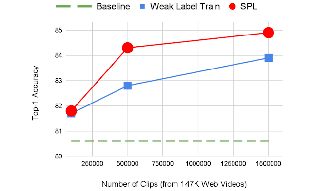
We also demonstrate that sampling more video clips from a given number of untrimmed videos can help improve the model performance. With a sufficient number of video clips available, SPL consistently outperforms weak label pre-training by providing enriched supervision.

As more clips are sampled from 147K videos, the label noise is increased gradually. SPL becomes more and more effective at utilizing the weakly-labeled clips to achieve better pre-training.

We visualize the visual concepts learned from SPL with attention visualization by applying Grad-CAM on the trained model. It is interesting to observe some meaningful “middle ground” concepts that can be learned by SPL.

Examples of attention visualization for SPL classes. Some meaningful “middle ground” concepts can be learned by SPL, such as mixing up the eggs and flour (left) and using the abseiling equipment (right).

Conclusion
We demonstrate that SPLs can provide enriched supervision for pre-training. SPL does not increase training complexity and can be treated as an off-the-shelf technique to integrate with teacher-student–based training frameworks. We believe this is a promising direction for discovering meaningful visual concepts by bridging weak labels and the knowledge distilled from teacher models. SPL has also demonstrated promising generalization to the image recognition domain and we expect future extensions that apply to tasks that have noise in labels. We have successfully applied SPL for Google Cloud Video AI where it has improved the accuracy of the action recognition models, helping users to better understand, search, and monetize their video content library.

Acknowledgements
We gratefully acknowledge the contributions of other co-authors, including Kunpeng Li, Xuehan Xiong, Chen-Yu Lee, Zhichao Lu, Yun Fu, Tomas Pfister. We also thank Debidatta Dwibedi, David A Ross, Chen Sun, Jonathan C. Stroud, and Wei Hua for their valuable comments and help on this work, and Tom Small for figure creation.

Source: Google AI Blog


Co-training Transformer with Videos and Images Improves Action Recognition

Action recognition has become a major focus area for the research community because many applications can benefit from improved modeling, such as video retrieval, video captioning, video question-answering, etc. Transformer-based approaches have recently demonstrated state-of-the-art performance on several benchmarks. While Transformer models require data to learn better visual priors compared to ConvNets, action recognition datasets are relatively small in scale. Large Transformer models are typically first trained on image datasets and later fine-tuned on a target action recognition dataset.

While the current pre-training and fine-tuning action recognition paradigm is straightforward and manifests strong empirical results, it may be overly restrictive for building general-purpose action-recognition models. Compared to a dataset like ImageNet that covers a large range of object recognition classes, action recognition datasets like Kinetics and Something-Something-v2 (SSv2) pertain to limited topics. For example, Kinetics include object-centric actions like “cliff diving” and “ice climbing’ while SSv2 contains object-agnostic activities like ’pretending to put something onto something else.’ As a result, we observed poor performance adapting an action recognition model that has been fine-tuned on one dataset to another disparate dataset.

Differences in objects and video backgrounds among datasets further exacerbate learning a general-purpose action recognition classification model. Despite the fact that video datasets may be increasing in size, prior work suggests significant data augmentation and regularization is necessary to achieve strong performance. This latter finding may indicate the model quickly overfits on the target dataset, and as a result, hinders its capacity to generalize to other action recognition tasks.

In “Co-training Transformer with Videos and Images Improves Action Recognition”, we propose a training strategy, named CoVeR, that leverages both image and video data to jointly learn a single general-purpose action recognition model. Our approach is buttressed by two main findings. First, disparate video datasets cover a diverse set of activities, and training them together in a single model could lead to a model that excels at a wide range of activities. Second, video is a perfect source for learning motion information, while images are great for exploiting structural appearance. Leveraging a diverse distribution of image examples may be beneficial in building robust spatial representations in video models. Concretely, CoVeR first pre-trains the model on an image dataset, and during fine-tuning, it simultaneously trains a single model on multiple video and image datasets to build robust spatial and temporal representations for a general-purpose video understanding model.

Architecture and Training Strategy
We applied the CoVeR approach to the recently proposed spatial-temporal video transformer, called TimeSFormer, that contains 24 layers of transformer blocks. Each block contains one temporal attention, one spatial attention, and one multilayer perceptron (MLP) layer. To learn from multiple video and image datasets, we adopt a multi-task learning paradigm and equip the action recognition model with multiple classification heads. We pre-train all non-temporal parameters on the large-scale JFT dataset. During fine-tuning, a batch of videos and images are sampled from multiple video and image datasets. The sampling rate is proportional to the size of the datasets. Each sample within the batch is processed by the TimeSFormer and then distributed to the corresponding classifier to get the predictions.

Compared with the standard training strategy, CoVeR has two advantages. First, as the model is directly trained on multiple datasets, the learned video representations are more general and can be directly evaluated on those datasets without additional fine-tuning. Second, Transformer-based models may easily overfit to a smaller video distribution, thus degrading the generalization of the learned representations. Training on multiple datasets mitigates this challenge by reducing the risk of overfitting.

CoVeR adopts a multi-task learning strategy trained on multiple datasets, each with their own classifier.

Benchmark Results
We evaluate the CoVeR approach to train on Kinetics-400 (K400), Kinetics-600 (K600), Kinetics-700 (K700), SomethingSomething-V2 (SSv2), and Moments-in-Time (MiT) datasets. Compared with other approaches — such as TimeSFormer, Video SwinTransformer, TokenLearner, ViViT, MoViNet, VATT, VidTr, and OmniSource — CoVeR established the new state-of-the-art on multiple datasets (shown below). Unlike previous approaches that train a dedicated model for one single dataset, a model trained by CoVeR can be directly applied to multiple datasets without further fine-tuning.

Model Pretrain Finetune K400 Accuracy
VATT AudioSet+Videos K400 82.1
Omnisource IG-Kinetics-65M K400 83.6
ViViT JFT-300M K400 85.4
Video SwinTrans   ImageNet21K+external   K400 86.8
CoVeR JFT-3B K400+SSv2+MiT+ImNet 87.2
Accuracy comparison on Kinetics-400 (K400) dataset.
Model Pretrain Finetune SSv2 Accuracy
TimeSFormer ImageNet21k SSv2 62.4
VidTr ImageNet21k SSv2 63.0
ViViT ImageNet21k SSv2 65.9
Video SwinTrans   ImageNet21K+external   SSv2 69.6
CoVeR JFT-3B K400+SSv2+MiT+ImNet 70.9
Accuracy comparison on SomethingSomething-V2 (SSv2) dataset.
Model Pretrain Finetune MiT Accuracy
ViViT ImageNet21k MiT 38.5
VidTr ImageNet21k SSv2 41.1
CoVeR JFT-3B K400+SSv2+MiT+ImNet 46.1
Accuracy comparison on Moments-in-Time (MiT) dataset.

Transfer Learning
We use transfer learning to further verify the video action recognition performance and compare with co-training on multiple datasets, results are summarized below. Specifically, we train on the source datasets, then fine-tune and evaluate on the target dataset.

We first consider K400 as the target dataset. CoVeR co-trained on SSv2 and MiT improves the top-1 accuracy on K400→K400 (where the model is trained on K400 and then fine-tuned on K400) by 1.3%, SSv2→K400 by 1.7%, and MiT→K400 by 0.4%. Similarly, we observe that by transferring to SSv2, CoVeR achieves 2%, 1.8%, and 1.1% improvement over SSv2→SSv2, K400→SSv2, and MiT→SSv2, respectively. The 1.2% and 2% performance improvement on K400 and SSv2 indicates that CoVeR co-trained on multiple datasets could learn better visual representations than the standard training paradigm, which is useful for downstream tasks.

Comparison of transfer learning the representation learned by CoVeR and standard training paradigm. A→B means the model is trained on dataset A and then fine-tuned on dataset B.

Conclusion
In this work, we present CoVeR, a training paradigm that jointly learns action recognition and object recognition tasks in a single model for the purpose of constructing a general-purpose action recognition framework. Our analysis indicates that it may be beneficial to integrate many video datasets into one multi-task learning paradigm. We highlight the importance of continuing to learn on image data during fine-tuning to maintain robust spatial representations. Our empirical findings suggest CoVeR can learn a single general-purpose video understanding model which achieves impressive performance across many action recognition datasets without an additional stage of fine-tuning on each downstream application.

Acknowledgements
We would like to thank Christopher Fifty, Wei Han, Andrew M. Dai, Ruoming Pang, and Fei Sha for preparation of the CoVeR paper, Yue Zhao, Hexiang Hu, Zirui Wang, Zitian Chen, Qingqing Huang, Claire Cui and Yonghui Wu for helpful discussions and feedbacks, and others on the Brain Team for support throughout this project.

Source: Google AI Blog


Nested Hierarchical Transformer: Towards Accurate, Data-Efficient, and Interpretable Visual Understanding

In visual understanding, the Visual Transformer (ViT) and its variants have received significant attention recently due to their superior performance on many core visual applications, such as image classification, object detection, and video understanding. The core idea of ViT is to utilize the power of self-attention layers to learn global relationships between small patches of images. However, the number of connections between patches increases quadratically with image size. Such a design has been observed to be data inefficient — although the original ViT can perform better than convolutional networks with hundreds of millions of images for pre-training, such a data requirement is not always practical, and it still underperforms compared to convolutional networks when given less data. Many are exploring to find more suitable architectural re-designs that can learn visual representations effectively, such as by adding convolutional layers and building hierarchical structures with local self-attention.

The principle of hierarchical structure is one of the core ideas in vision models, where bottom layers learn more local object structures on the high-dimensional pixel space and top layers learn more abstracted and high-level knowledge at low-dimensional feature space. Existing ViT-based methods focus on designing a variety of modifications inside self-attention layers to achieve such a hierarchy, but while these offer promising performance improvements, they often require substantial architectural re-designs. Moreover, these approaches lack an interpretable design, so it is difficult to explain the inner-workings of trained models.

To address these challenges, in “Nested Hierarchical Transformer: Towards Accurate, Data-Efficient and Interpretable Visual Understanding”, we present a rethinking of existing hierarchical structure–driven designs, and provide a novel and orthogonal approach to significantly simplify them. The central idea of this work is to decouple feature learning and feature abstraction (pooling) components: nested transformer layers encode visual knowledge of image patches separately, and then the processed information is aggregated. This process is repeated in a hierarchical manner, resulting in a pyramid network structure. The resulting architecture achieves competitive results on ImageNet and outperforms results on data-efficient benchmarks. We have shown such a design can meaningfully improve data efficiency with faster convergence and provide valuable interpretability benefits. Moreover, we introduce GradCAT, a new technique for interpreting the decision process of a trained model at inference time.

Architecture Design
The overall architecture is simple to implement by adding just a few lines of Python code to the source code of the original ViT. The original ViT architecture divides an input image into small patches, projects pixels of each patch to a vector with predefined dimension, and then feeds the sequences of all vectors to the overall ViT architecture containing multiple stacked identical transformer layers. While every layer in ViT processes information of the whole image, with this new method, stacked transformer layers are used to process only a region (i.e., block) of the image containing a few spatially adjacent image patches. This step is independent for each block and is also where feature learning occurs. Finally, a new computational layer called block aggregation then combines all of the spatially adjacent blocks. After each block aggregation, the features corresponding to four spatially adjacent blocks are fed to another module with a stack of transformer layers, which then process those four blocks jointly. This design naturally builds a pyramid hierarchical structure of the network, where bottom layers can focus on local features (such as textures) and upper layers focus on global features (such as object shape) at reduced dimensionality thanks to the block aggregation.

A visualization of the network processing an image: Given an input image, the network first partitions images into blocks, where each block contains 4 image patches. Image patches in every block are linearly projected as vectors and processed by a stack of identical transformer layers. Then the proposed block aggregation layer aggregates information from each block and reduces its spatial size by 4 times. The number of blocks is reduced to 1 at the top hierarchy and classification is conducted after the output of it.

Interpretability
This architecture has a non-overlapping information processing mechanism, independent at every node. This design resembles a decision tree-like structure, which manifests unique interpretability capabilities because every tree node contains independent information of an image block that is being received by its parent nodes. We can trace the information flow through the nodes to understand the importance of each feature. In addition, our hierarchical structure retains the spatial structure of images throughout the network, leading to learned spatial feature maps that are effective for interpretation. Below we showcase two kinds of visual interpretability.

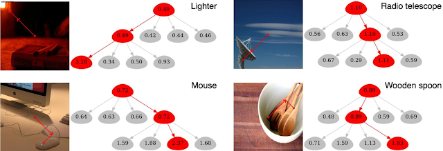
First, we present a method to interpret the trained model on test images, called gradient-based class-aware tree-traversal (GradCAT). GradCAT traces the feature importance of each block (a tree node) from top to bottom of the hierarchy structure. The main idea is to find the most valuable traversal from the root node at the top layer to a child node at the bottom layer that contributes the most to the classification outcomes. Since each node processes information from a certain region of the image, such traversal can be easily mapped to the image space for interpretation (as shown by the overlaid dots and lines in the image below).

The following is an example of the model's top-4 predictions and corresponding interpretability results on the left input image (containing 4 animals). As shown below, GradCAT highlights the decision path along the hierarchical structure as well as the corresponding visual cues in local image regions on the images.

Given the left input image (containing four objects), the figure visualizes the interpretability results of the top-4 prediction classes. The traversal locates the model decision path along the tree and simultaneously locates the corresponding image patch (shown by the dotted line on images) that has the highest impact to the predicted target class.

Moreover, the following figures visualize results on the ImageNet validation set and show how this approach enables some intuitive observations. For instance, the example of the lighter below (upper left panel) is particularly interesting because the ground truth class — lighter/matchstick — actually defines the bottom-right matchstick object, while the most salient visual features (with the highest node values) are actually from the upper-left red light, which conceptually shares visual cues with a lighter. This can also be seen from the overlaid red lines, which indicate the image patches with the highest impact on the prediction. Thus, although the visual cue is a mistake, the output prediction is correct. In addition, the four child nodes of the wooden spoon below have similar feature importance values (see numbers visualized in the nodes; higher indicates more importance), which is because the wooden texture of the table is similar to that of the spoon.

Visualization of the results obtained by the proposed GradCAT. Images are from the ImageNet validation dataset.

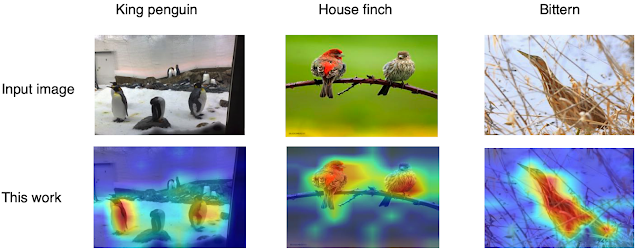
Second, different from the original ViT, our hierarchical architecture retains spatial relationships in learned representations. The top layers output low-resolution features maps of input images, enabling the model to easily perform attention-based interpretation by applying Class Attention Map (CAM) on the learned representations at the top hierarchical level. This enables high-quality weakly-supervised object localization with just image-level labels. See the following figure for examples.

Visualization of CAM-based attention results. Warmer colors indicate higher attention. Images are from the ImageNet validation dataset.

Convergence Advantages
With this design, feature learning only happens at local regions independently, and feature abstraction happens inside the aggregation function. This design and simple implementation is general enough for other types of visual understanding tasks beyond classification. It also improves the model convergence speed greatly, significantly reducing the training time to reach the desired maximum accuracy.

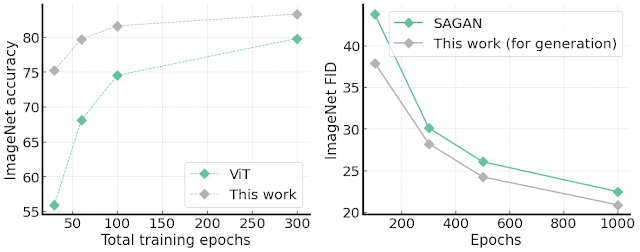
We validate this advantage in two ways. First, we compare the ViT structure on the ImageNet accuracy with a different number of total training epochs. The results are shown on the left side of the figure below, demonstrating much faster convergence than the original ViT, e.g., around 20% improvement in accuracy over ViT with 30 total training epochs.

Second, we modify the architecture to conduct unconditional image generation tasks, since training ViT-based models for image generation tasks is challenging due to convergence and speed issues. Creating such a generator is straightforward by transposing the proposed architecture: the input is an embedding vector, the output is a full image in RGB channels, and the block aggregation is replaced by a block de-aggregation component supported by Pixel Shuffling. Surprisingly, we find our generator is easy to train and demonstrates faster convergence speed, as well as better FID score (which measures how similar generated images are to real ones), than the capacity-comparable SAGAN.

Left: ImageNet accuracy given different number of total training epochs compared with standard ViT architecture. Right: ImageNet 64x64 image generation FID scores (lower is better) with single 1000-epoch training. On both tasks, our method shows better convergence speed.

Conclusion
In this work we demonstrate the simple idea that decoupled feature learning and feature information extraction in this nested hierarchy design leads to better feature interpretability through a new gradient-based class-aware tree traversal method. Moreover, the architecture improves convergence on not only classification tasks but also image generation tasks. The proposed idea is focusing on aggregation function and thereby is orthogonal to advanced architecture design for self-attention. We hope this new research encourages future architecture designers to explore more interpretable and data-efficient ViT-based models for visual understanding, like the adoption of this work for high-resolution image generation. We have also released the source code for the image classification portion of this work.

Acknowledgements
We gratefully acknowledge the contributions of other co-authors, including Han Zhang, Long Zhao, Ting Chen, Sercan Arik, Tomas Pfister. We also thank Xiaohua Zhai, Jeremy Kubica, Kihyuk Sohn, and Madeleine Udell for the valuable feedback of the work.

Source: Google AI Blog


Robot See, Robot Do

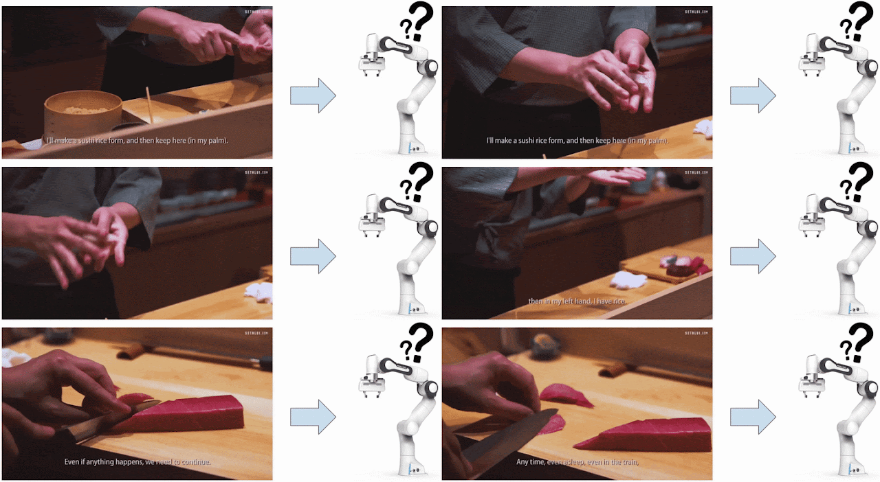
People learn to do things by watching others — from mimicking new dance moves, to watching YouTube cooking videos. We’d like robots to do the same, i.e., to learn new skills by watching people do things during training. Today, however, the predominant paradigm for teaching robots is to remote control them using specialized hardware for teleoperation and then train them to imitate pre-recorded demonstrations. This limits both who can provide the demonstrations (programmers & roboticists) and where they can be provided (lab settings). If robots could instead self-learn new tasks by watching humans, this capability could allow them to be deployed in more unstructured settings like the home, and make it dramatically easier for anyone to teach or communicate with them, expert or otherwise. Perhaps one day, they might even be able to use Youtube videos to grow their collection of skills over time.

Our motivation is to have robots watch people do tasks, naturally with their hands, and then use that data as demonstrations for learning. Video by Teh Aik Hui and Nathaniel Lim. License: CC-BY

However, an obvious but often overlooked problem is that a robot is physically different from a human, which means it often completes tasks differently than we do. For example, in the pen manipulation task below, the hand can grab all the pens together and quickly transfer them between containers, whereas the two-fingered gripper must transport one at a time. Prior research assumes that humans and robots can do the same task similarly, which makes manually specifying one-to-one correspondences between human and robot actions easy. But with stark differences in physique, defining such correspondences for seemingly easy tasks can be surprisingly difficult and sometimes impossible.

Physically different end-effectors (i.e., “grippers”) (i.e., the part that interacts with the environment) induce different control strategies when solving the same task. Left: The hand grabs all pens and quickly transfers them between containers. Right: The two-fingered gripper transports one pen at a time.

In “XIRL: Cross-Embodiment Inverse RL”, presented as an oral paper at CoRL 2021, we explore these challenges further and introduce a self-supervised method for Cross-embodiment Inverse Reinforcement Learning (XIRL). Rather than focusing on how individual human actions should correspond to robot actions, XIRL learns the high-level task objective from videos, and summarizes that knowledge in the form of a reward function that is invariant to embodiment differences, such as shape, actions and end-effector dynamics. The learned rewards can then be used together with reinforcement learning to teach the task to agents with new physical embodiments through trial and error. Our approach is general and scales autonomously with data — the more embodiment diversity presented in the videos, the more invariant and robust the reward functions become. Experiments show that our learned reward functions lead to significantly more sample efficient (roughly 2 to 4 times) reinforcement learning on new embodiments compared to alternative methods. To extend and build on our work, we are releasing an accompanying open-source implementation of our method along with X-MAGICAL, our new simulated benchmark for cross-embodiment imitation.

Cross-Embodiment Inverse Reinforcement Learning (XIRL)
The underlying observation in this work is that in spite of the many differences induced by different embodiments, there still exist visual cues that reflect progression towards a common task objective. For example, in the pen manipulation task above, the presence of pens in the cup but not the mug, or the absence of pens on the table, are key frames that are common to different embodiments and indirectly provide cues for how close to being complete a task is. The key idea behind XIRL is to automatically discover these key moments in videos of different length and cluster them meaningfully to encode task progression. This motivation shares many similarities with unsupervised video alignment research, from which we can leverage a method called Temporal Cycle Consistency (TCC), which aligns videos accurately while learning useful visual representations for fine-grained video understanding without requiring any ground-truth correspondences.

We leverage TCC to train an encoder to temporally align video demonstrations of different experts performing the same task. The TCC loss tries to maximize the number of cycle-consistent frames (or mutual nearest-neighbors) between pairs of sequences using a differentiable formulation of soft nearest-neighbors. Once the encoder is trained, we define our reward function as simply the negative Euclidean distance between the current observation and the goal observation in the learned embedding space. We can subsequently insert the reward into a standard MDP and use an RL algorithm to learn the demonstrated behavior. Surprisingly, we find that this simple reward formulation is effective for cross-embodiment imitation.

XIRL self-supervises reward functions from expert demonstrations using temporal cycle consistency (TCC), then uses them for downstream reinforcement learning to learn new skills from third-person demonstrations.

X-MAGICAL Benchmark
To evaluate the performance of XIRL and baseline alternatives (e.g., TCN, LIFS, Goal Classifier) in a consistent environment, we created X-MAGICAL, which is a simulated benchmark for cross-embodiment imitation. X-MAGICAL features a diverse set of agent embodiments, with differences in their shapes and end-effectors, designed to solve tasks in different ways. This leads to differences in execution speeds and state-action trajectories, which poses challenges for current imitation learning techniques, e.g., ones that use time as a heuristic for weak correspondences between two trajectories. The ability to generalize across embodiments is precisely what X-MAGICAL evaluates.

The SweepToTop task we considered for our experiments is a simplified 2D equivalent of a common household robotic sweeping task, where an agent has to push three objects into a goal zone in the environment. We chose this task specifically because its long-horizon nature highlights how different agent embodiments can generate entirely different trajectories (shown below). X-MAGICAL features a Gym API and is designed to be easily extendable to new tasks and embodiments. You can try it out today with pip install x-magical.

Different agent shapes in the SweepToTop task in the X-MAGICAL benchmark need to use different strategies to reposition objects into the target area (pink), i.e., to “clear the debris”. For example, the long-stick can clear them all in one fell swoop, whereas the short-stick needs to do multiple consecutive back-and-forths.
Left: Heatmap of state visitation for each embodiment across all expert demonstrations. Right: Examples of expert trajectories for each embodiment.

Highlights
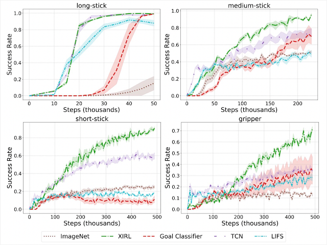
In our first set of experiments, we checked whether our learned embodiment-invariant reward function can enable successful reinforcement learning, when the expert demonstrations are provided through the agent itself. We find that XIRL significantly outperforms alternative methods especially on the tougher agents (e.g., short-stick and gripper).

Same-embodiment setting: Comparison of XIRL with baseline reward functions, using SAC for RL policy learning. XIRL is roughly 2 to 4 times more sample efficient than some of the baselines on the harder agents (short-stick and gripper).

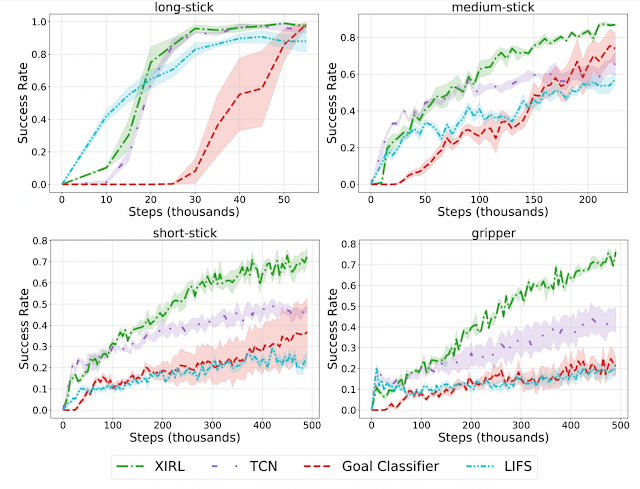
We also find that our approach shows great potential for learning reward functions that generalize to novel embodiments. For instance, when reward learning is performed on embodiments that are different from the ones on which the policy is trained, we find that it results in significantly more sample efficient agents compared to the same baselines. Below, in the gripper subplot (bottom right) for example, the reward is first learned on demonstration videos from long-stick, medium-stick and short-stick, after which the reward function is used to train the gripper agent.

Cross-embodiment setting: XIRL performs favorably when compared with other baseline reward functions, trained on observation-only demonstrations from different embodiments. Each agent (long-stick, medium-stick, short-stick, gripper) had its reward trained using demonstrations from the other three embodiments.

We also find that we can train on real-world human demonstrations, and use the learned reward to train a Sawyer arm in simulation to push a puck to a designated target zone. In these experiments as well, our method outperforms baseline alternatives. For example, our XIRL variant trained only on the real-world demonstrations (purple in the plots below) reaches 80% of the total performance roughly 85% faster than the RLV baseline (orange).

What Do The Learned Reward Functions Look Like?
To further explore the qualitative nature of our learned rewards in more challenging real-world scenarios, we collect a dataset of the pen transfer task using various household tools.

Below, we show rewards extracted from a successful (top) and unsuccessful (bottom) demonstration. Both demonstrations follow a similar trajectory at the start of the task execution. The successful one nets a high reward for placing the pens consecutively into the mug then into the glass cup, while the unsuccessful one obtains a low reward because it drops the pens outside the glass cup towards the end of the execution (orange circle). These results are promising because they show that our learned encoder can represent fine-grained visual differences relevant to a task.

Conclusion
We highlighted XIRL, our approach to tackling the cross-embodiment imitation problem. XIRL learns an embodiment-invariant reward function that encodes task progress using a temporal cycle-consistency objective. Policies learned using our reward functions are significantly more sample-efficient than baseline alternatives. Furthermore, the reward functions do not require manually paired video frames between the demonstrator and the learner, giving them the ability to scale to an arbitrary number of embodiments or experts with varying skill levels. Overall, we are excited about this direction of work, and hope that our benchmark promotes further research in this area. For more details, please check out our paper and download the code from our GitHub repository.

Acknowledgments
Kevin and Andy summarized research performed together with Pete Florence, Jonathan Tompson, Jeannette Bohg (faculty at Stanford University) and Debidatta Dwibedi. All authors would additionally like to thank Alex Nichol, Nick Hynes, Sean Kirmani, Brent Yi, Jimmy Wu, Karl Schmeckpeper and Minttu Alakuijala for fruitful technical discussions, and Sam Toyer for invaluable help with setting up the simulated benchmark.

Source: Google AI Blog


Unlocking the Full Potential of Datacenter ML Accelerators with Platform-Aware Neural Architecture Search

Continuing advances in the design and implementation of datacenter (DC) accelerators for machine learning (ML), such as TPUs and GPUs, have been critical for powering modern ML models and applications at scale. These improved accelerators exhibit peak performance (e.g., FLOPs) that is orders of magnitude better than traditional computing systems. However, there is a fast-widening gap between the available peak performance offered by state-of-the-art hardware and the actual achieved performance when ML models run on that hardware.

One approach to address this gap is to design hardware-specific ML models that optimize both performance (e.g., throughput and latency) and model quality. Recent applications of neural architecture search (NAS), an emerging paradigm to automate the design of ML model architectures, have employed a platform-aware multi-objective approach that includes a hardware performance objective. While this approach has yielded improved model performance in practice, the details of the underlying hardware architecture are opaque to the model. As a result, there is untapped potential to build full capability hardware-friendly ML model architectures, with hardware-specific optimizations, for powerful DC ML accelerators.

In “Searching for Fast Model Families on Datacenter Accelerators”, published at CVPR 2021, we advanced the state of the art of hardware-aware NAS by automatically adapting model architectures to the hardware on which they will be executed. The approach we propose finds optimized families of models for which additional hardware performance gains cannot be achieved without loss in model quality (called Pareto optimization). To accomplish this, we infuse a deep understanding of hardware architecture into the design of the NAS search space for discovery of both single models and model families. We provide quantitative analysis of the performance gap between hardware and traditional model architectures and demonstrate the advantages of using true hardware performance (i.e., throughput and latency), instead of the performance proxy (FLOPs), as the performance optimization objective. Leveraging this advanced hardware-aware NAS and building upon the EfficientNet architecture, we developed a family of models, called EfficientNetX, that demonstrate the effectiveness of this approach for Pareto-optimized ML models on TPUs and GPUs.

Platform-Aware NAS for DC ML Accelerators
To achieve high performance, ML models need to adapt to modern ML accelerators. Platform-aware NAS integrates knowledge of the hardware accelerator properties into all three pillars of NAS: (i) the search objectives; (ii) the search space; and (iii) the search algorithm (shown below). We focus on the new search space because it contains the building blocks needed to compose the models and is the key link between the ML model architectures and accelerator hardware architectures.

We construct TPU/GPU specialized search spaces with TPU/GPU-friendly operations to infuse hardware awareness into NAS. For example, a key adaptation is maximizing parallelism to ensure different hardware components inside the accelerators work together as efficiently as possible. This includes the matrix multiplication units (MXUs) in TPUs and the TensorCore in GPUs for matrix/tensor computation, as well as the vector processing units (VPUs) in TPUs and CUDA cores in GPUs for vector processing. Maximizing model arithmetic intensity (i.e., optimizing the parallelism between computation and operations on the high bandwidth memory) is also critical to achieve top performance. To tap into the full potential of the hardware, it is crucial for ML models to achieve high parallelism inside and across these hardware components.

Overview of platform-aware NAS on TPUs/GPUs, highlighting the search space and search objectives.

Advanced platform-aware NAS has an optimized search space containing a set of complementary techniques to holistically improve parallelism for ML model execution on TPUs and GPUs:

  1. It uses specialized tensor reshaping techniques to maximize the parallelism in the MXUs / TensorCores.
  2. It dynamically selects different activation functions depending on matrix operation types to ensure overlapping of vector and matrix/tensor processing.
  3. It employs hybrid convolutions and a novel fusion strategy to strike a balance between total compute and arithmetic intensity to ensure that computation and memory access happens in parallel and to reduce the contention on VPUs / CUDA cores.
  4. With latency-aware compound scaling (LACS), which uses hardware performance instead of FLOPs as the performance objective to search for model depth, width and resolutions, we ensure parallelism at all levels for the entire model family on the Pareto-front.

EfficientNet-X: Platform-Aware NAS-Optimized Computer Vision Models for TPUs and GPUs
Using this approach to platform-aware NAS, we have designed EfficientNet-X, an optimized computer vision model family for TPUs and GPUs. This family builds upon the EfficientNet architecture, which itself was originally designed by traditional multi-objective NAS without true hardware-awareness as the baseline. The resulting EfficientNet-X model family achieves an average speedup of ~1.5x–2x over EfficientNet on TPUv3 and GPUv100, respectively, with comparable accuracy.

In addition to the improved speeds, EfficientNet-X has shed light on the non-proportionality between FLOPs and true performance. Many think FLOPs are a good ML performance proxy (i.e., FLOPs and performance are proportional), but they are not. While FLOPs are a good performance proxy for simple hardware such as scalar machines, they can exhibit a margin of error of up to 400% on advanced matrix/tensor machines. For example, because of its hardware-friendly model architecture, EfficientNet-X requires ~2x more FLOPs than EfficientNet, but is ~2x faster on TPUs and GPUs.

EfficientNet-X family achieves 1.5x–2x speedup on average over the state-of-the-art EfficientNet family, with comparable accuracy on TPUv3 and GPUv100.

Self-Driving ML Model Performance on New Accelerator Hardware Platforms
Platform-aware NAS exposes the inner workings of the hardware and leverages these properties when designing hardware-optimized ML models. In a sense, the “platform-awareness” of the model is a “gene” that preserves knowledge of how to optimize performance for a hardware family, even on new generations, without the need to redesign the models. For example, TPUv4i delivers up to 3x higher peak performance (FLOPS) than its predecessor TPUv2, but EfficientNet performance only improves by 30% when migrating from TPUv2 to TPUv4i. In comparison, EfficientNet-X retains its platform-aware properties even on new hardware and achieves a 2.6x speedup when migrating from TPUv2 to TPUv4i, utilizing almost all of the 3x peak performance gain expected when upgrading between the two generations.

Hardware peak performance ratio of TPUv2 to TPUv4i and the geometric mean speedup of EfficientNet-X and EfficientNet families, respectively, when migrating from TPUv2 to TPUv4i.

Conclusion and Future Work
We demonstrate how to improve the capabilities of platform-aware NAS for datacenter ML accelerators, especially TPUs and GPUs. Both platform-aware NAS and the EfficientNet-X model family have been deployed in production and materialize up to ~40% efficiency gains and significant quality improvements for various internal computer vision projects across Google. Additionally, because of its deep understanding of accelerator hardware architecture, platform-aware NAS was able to identify critical performance bottlenecks on TPUv2-v4i architectures and has enabled design enhancements to future TPUs with significant potential performance uplift. As next steps, we are working on expanding platform-aware NAS’s capabilities to the ML hardware and model design beyond computer vision.

Acknowledgements
Special thanks to our co-authors: Mingxing Tan, Ruoming Pang, Andrew Li, Liqun Cheng, Quoc Le. We also thank many collaborators including Jeff Dean, David Patterson, Shengqi Zhu, Yun Ni, Gang Wu, Tao Chen, Xin Li, Yuan Qi, Amit Sabne, Shahab Kamali, and many others from the broad Google research and engineering teams who helped on the research and the subsequent broad production deployment of platform-aware NAS.

Source: Google AI Blog


Scaling Vision with Sparse Mixture of Experts

Advances in deep learning over the last few decades have been driven by a few key elements. With a small number of simple but flexible mechanisms (i.e., inductive biases such as convolutions or sequence attention), increasingly large datasets, and more specialized hardware, neural networks can now achieve impressive results on a wide range of tasks, such as image classification, machine translation, and protein folding prediction.

However, the use of large models and datasets comes at the expense of significant computational requirements. Yet, recent works suggest that large model sizes might be necessary for strong generalization and robustness, so training large models while limiting resource requirements is becoming increasingly important. One promising approach involves the use of conditional computation: rather than activating the whole network for every single input, different parts of the model are activated for different inputs. This paradigm has been featured in the Pathways vision and recent works on large language models, while it has not been well explored in the context of computer vision.

In “Scaling Vision with Sparse Mixture of Experts”, we present V-MoE, a new vision architecture based on a sparse mixture of experts, which we then use to train the largest vision model to date. We transfer V-MoE to ImageNet and demonstrate matching state-of-the-art accuracy while using about 50% fewer resources than models of comparable performance. We have also open-sourced the code to train sparse models and provided several pre-trained models.

Vision Mixture of Experts (V-MoEs)
Vision Transformers (ViT) have emerged as one of the best architectures for vision tasks. ViT first partitions an image into equally-sized square patches. These are called tokens, a term inherited from language models. Still, compared to the largest language models, ViT models are several orders of magnitude smaller in terms of number of parameters and compute.

To massively scale vision models, we replace some dense feedforward layers (FFN) in the ViT architecture with a sparse mixture of independent FFNs (which we call experts). A learnable router layer selects which experts are chosen (and how they are weighted) for every individual token. That is, different tokens from the same image may be routed to different experts. Each token is only routed to at most K (typically 1 or 2) experts, among a total of E experts (in our experiments, E is typically 32). This allows scaling the model’s size while keeping its computation per token roughly constant. The figure below shows the structure of the encoder blocks in more detail.

V-MoE Transformer Encoder block.

Experimental Results
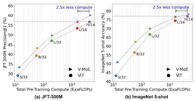
We first pre-train the model once on JFT-300M, a large dataset of images. The left plot below shows our pre-training results for models of all sizes: from the small S/32 to the huge H/14.

We then transfer the model to new downstream tasks (such as ImageNet), by using a new head (the last layer in a model). We explore two transfer setups: either fine-tuning the entire model on all available examples of the new task, or freezing the pre-trained network and tuning only the new head using a few examples (known as few-shot transfer). The right plot in the figure below summarizes our transfer results to ImageNet, training on only 5 images per class (called 5-shot transfer).

JFT-300M Precision@1 and ImageNet 5-shot accuracy. Colors represent different ViT variants and markers represent either standard ViT (●), or V-MoEs (▸) with expert layers on the last n even blocks. We set n=2 for all models, except V-MoE-H where n=5. Higher indicates better performance, with more efficient models being to the left.

In both cases, the sparse model strongly outperforms its dense counterpart at a given amount of training compute (shown by the V-MoE line being above the ViT line), or achieves similar performance much faster (shown by the V-MoE line being to the left of the ViT line).

To explore the limits of vision models, we trained a 15-billion parameter model with 24 MoE layers (out of 48 blocks) on an extended version of JFT-300M. This massive model — the largest to date in vision as far as we know — achieved 90.35% test accuracy on ImageNet after fine-tuning, near the current state-of-the-art.

Priority Routing
In practice, due to hardware constraints, it is not efficient to use buffers with a dynamic size, so models typically use a pre-defined buffer capacity for each expert. Assigned tokens beyond this capacity are dropped and not processed once the expert becomes "full". As a consequence, higher capacities yield higher accuracy, but they are also more computationally expensive.

We leverage this implementation constraint to make V-MoEs faster at inference time. By decreasing the total combined buffer capacity below the number of tokens to be processed, the network is forced to skip processing some tokens in the expert layers. Instead of choosing the tokens to skip in some arbitrary fashion (as previous works did), the model learns to sort tokens according to an importance score. This maintains high quality predictions while saving a lot of compute. We refer to this approach as Batch Priority Routing (BPR), illustrated below.

Under high capacity, both vanilla and priority routing work well as all patches are processed. However, when the buffer size is reduced to save compute, vanilla routing selects arbitrary patches to process, often leading to poor predictions. BPR smartly prioritizes important patches resulting in better predictions at lower computational costs.

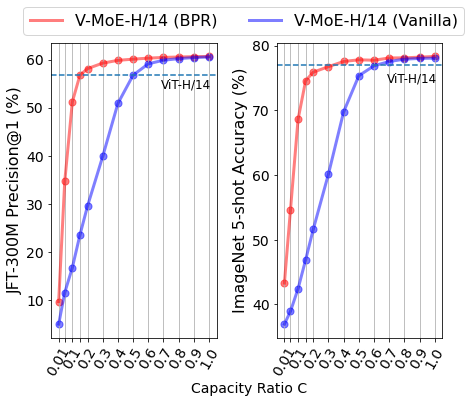
Dropping the right tokens turns out to be essential to deliver high-quality and more efficient inference predictions. When the expert capacity decreases, performance quickly decreases with the vanilla routing mechanism. Conversely, BPR is much more robust to low capacities.

Performance versus inference capacity buffer size (or ratio) C for a V-MoE-H/14 model with K=2. Even for large C’s, BPR improves performance; at low C the difference is quite significant. BPR is competitive with dense models (ViT-H/14) by processing only 15-30% of the tokens.

Overall, we observed that V-MoEs are highly flexible at inference time: for instance, one can decrease the number of selected experts per token to save time and compute, without any further training on the model weights.

Exploring V-MoEs
Because much is yet to be discovered about the internal workings of sparse networks, we also explored the routing patterns of the V-MoE.

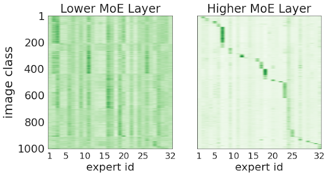
One hypothesis is that routers would learn to discriminate and assign tokens to experts based on some semantic grounds (the “car” expert, the “animal” experts, and so on). To test this, below we show plots for two different MoE layers (a very early-on one, and another closer to the head). The x-axis corresponds to each of the 32 experts, and the y-axis shows the ID of the image classes (from 1 to 1000). Each entry in the plot shows how often an expert was selected for tokens corresponding to the specific image class, with darker colors indicating higher frequency. While in the early layers there is little correlation, later in the network, each expert receives and processes tokens from only a handful of classes. Therefore, we can conclude that some semantic clustering of the patches emerges in the deeper layers of the network.

Higher routing decisions correlate with image classes. We show two MoE layers of a V-MoE-H/14. The x-axis corresponds to the 32 experts in a layer. The y-axis are the 1000 ImageNet classes; orderings for both axes are different across plots (to highlight correlations). For each pair (expert e, class c) we show the average routing weight for the tokens corresponding to all images with class c for that particular expert e.

Final Thoughts
We train very large vision models using conditional computation, delivering significant improvements in representation and transfer learning for relatively little training cost. Alongside V-MoE, we introduced BPR, which requires the model to process only the most useful tokens in the expert layers.

We believe this is just the beginning of conditional computation at scale for computer vision; extensions include multi-modal and multi-task models, scaling up the expert count, and improving transfer of the representations produced by sparse models. Heterogeneous expert architectures and conditional variable-length routes are also promising directions. Sparse models can especially help in data rich domains such as large-scale video modeling. We hope our open-source code and models help attract and engage researchers new to this field.

Acknowledgments
We thank our co-authors: Basil Mustafa, Maxim Neumann, Rodolphe Jenatton, André Susano Pinto, Daniel Keysers, and Neil Houlsby. We thank Alex Kolesnikov, Lucas Beyer, and Xiaohua Zhai for providing continuous help and details about scaling ViT models. We are also grateful to Josip Djolonga, Ilya Tolstikhin, Liam Fedus, and Barret Zoph for feedback on the paper; James Bradbury, Roy Frostig, Blake Hechtman, Dmitry Lepikhin, Anselm Levskaya, and Parker Schuh for invaluable support helping us run our JAX models efficiently on TPUs; and many others from the Brain team for their support. Finally, we would also like to thank and acknowledge Tom Small for the awesome animated figure used in this post.

Source: Google AI Blog


Improving Vision Transformer Efficiency and Accuracy by Learning to Tokenize

Transformer models consistently obtain state-of-the-art results in computer vision tasks, including object detection and video classification. In contrast to standard convolutional approaches that process images pixel-by-pixel, the Vision Transformers (ViT) treat an image as a sequence of patch tokens (i.e., a smaller part, or “patch”, of an image made up of multiple pixels). This means that at every layer, a ViT model recombines and processes patch tokens based on relations between each pair of tokens, using multi-head self-attention. In doing so, ViT models have the capability to construct a global representation of the entire image.

At the input-level, the tokens are formed by uniformly splitting the image into multiple segments, e.g., splitting an image that is 512 by 512 pixels into patches that are 16 by 16 pixels. At the intermediate levels, the outputs from the previous layer become the tokens for the next layer. In the case of videos, video ‘tubelets’ such as 16x16x2 video segments (16x16 images over 2 frames) become tokens. The quality and quantity of the visual tokens decide the overall quality of the Vision Transformer.

The main challenge in many Vision Transformer architectures is that they often require too many tokens to obtain reasonable results. Even with 16x16 patch tokenization, for instance, a single 512x512 image corresponds to 1024 tokens. For videos with multiple frames, that results in tens of thousands of tokens needing to be processed at every layer. Considering that the Transformer computation increases quadratically with the number of tokens, this can often make Transformers intractable for larger images and longer videos. This leads to the question: is it really necessary to process that many tokens at every layer?

In “TokenLearner: What Can 8 Learned Tokens Do for Images and Videos?”, an earlier version of which is presented at NeurIPS 2021, we show that adaptively generating a smaller number of tokens, rather than always relying on tokens formed by uniform splitting, enables Vision Transformers to run much faster and perform better. TokenLearner is a learnable module that takes an image-like tensor (i.e., input) and generates a small set of tokens. This module could be placed at various different locations within the model of interest, significantly reducing the number of tokens to be handled in all subsequent layers. The experiments demonstrate that having TokenLearner saves memory and computation by half or more without damaging classification performance, and because of its ability to adapt to inputs, it even increases the accuracy.

The TokenLearner
We implement TokenLearner using a straightforward spatial attention approach. In order to generate each learned token, we compute a spatial attention map highlighting regions-of-importance (using convolutional layers or MLPs). Such a spatial attention map is then applied to the input to weight each region differently (and discard unnecessary regions), and the result is spatially pooled to generate the final learned tokens. This is repeated multiple times in parallel, resulting in a few (~10) tokens out of the original input. This can also be viewed as performing a soft-selection of the pixels based on the weight values, followed by global average pooling. Note that the functions to compute the attention maps are governed by different sets of learnable parameters, and are trained in an end-to-end fashion. This allows the attention functions to be optimized in capturing different spatial information in the input. The figure below illustrates the process.

The TokenLearner module learns to generate a spatial attention map for each output token, and uses it to abstract the input to tokenize. In practice, multiple spatial attention functions are learned, are applied to the input, and generate different token vectors in parallel.

As a result, instead of processing fixed, uniformly tokenized inputs, TokenLearner enables models to process a smaller number of tokens that are relevant to the specific recognition task. That is, (1) we enable adaptive tokenization so that the tokens can be dynamically selected conditioned on the input, and (2) this effectively reduces the total number of tokens, greatly reducing the computation performed by the network. These dynamically and adaptively generated tokens can be used in standard transformer architectures such as ViT for images and ViViT for videos.

Where to Place TokenLearner
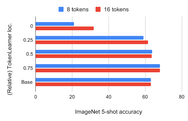
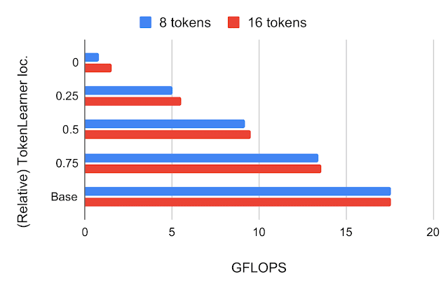
After building the TokenLearner module, we had to determine where to place it. We first tried placing it at different locations within the standard ViT architecture with 224x224 images. The number of tokens TokenLearner generated was 8 and 16, much less than 196 or 576 tokens the standard ViTs use. The below figure shows ImageNet few-shot classification accuracies and FLOPS of the models with TokenLearner inserted at various relative locations within ViT B/16, which is the base model with 12 attention layers operating on 16x16 patch tokens.

Top: ImageNet 5-shot transfer accuracy with JFT 300M pre-training, with respect to the relative TokenLearner locations within ViT B/16. Location 0 means TokenLearner is placed before any Transformer layer. Base is the original ViT B/16. Bottom: Computation, measured in terms of billions of floating point operations (GFLOPS), per relative TokenLearner location.

We found that inserting TokenLearner after the initial quarter of the network (at 1/4) achieves almost identical accuracies as the baseline, while reducing the computation to less than a third of the baseline. In addition, placing TokenLearner at the later layer (after 3/4 of the network) achieves even better performance compared to not using TokenLearner while performing faster, thanks to its adaptiveness. Due to the large difference between the number of tokens before and after TokenLearner (e.g., 196 before and 8 after), the relative computation of the transformers after the TokenLearner module becomes almost negligible.

Comparing Against ViTs
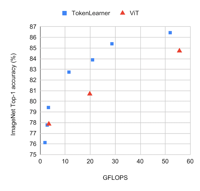
We compared the standard ViT models with TokenLearner against those without it while following the same setting on ImageNet few-shot transfer. TokenLearner was placed in the middle of each ViT model at various locations such as at 1/2 and at 3/4. The below figure shows the performance/computation trade-off of the models with and without TokenLearner.

Performance of various versions of ViT models with and without TokenLearner, on ImageNet classification. The models were pre-trained with JFT 300M. The closer a model is to the top-left of each graph the better, meaning that it runs faster and performs better. Observe how TokenLearner models perform better than ViT in terms of both accuracy and computation.

We also inserted TokenLearner within larger ViT models, and compared them against the giant ViT G/14 model. Here, we applied TokenLearner to ViT L/10 and L/8, which are the ViT models with 24 attention layers taking 10x10 (or 8x8) patches as initial tokens. The below figure shows that despite using many fewer parameters and less computation, TokenLearner performs comparably to the giant G/14 model with 48 layers.

Left: Classification accuracy of large-scale TokenLearner models compared to ViT G/14 on ImageNet datasets. Right: Comparison of the number of parameters and FLOPS.

High-Performing Video Models
Video understanding is one of the key challenges in computer vision, so we evaluated TokenLearner on multiple video classification datasets. This was done by adding TokenLearner into Video Vision Transformers (ViViT), which can be thought of as a spatio-temporal version of ViT. TokenLearner learned 8 (or 16) tokens per timestep.

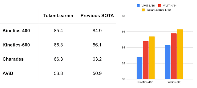
When combined with ViViT, TokenLearner obtains state-of-the-art (SOTA) performance on multiple popular video benchmarks, including Kinetics-400, Kinetics-600, Charades, and AViD, outperforming the previous Transformer models on Kinetics-400 and Kinetics-600 as well as previous CNN models on Charades and AViD.

Models with TokenLearner outperform state-of-the-art on popular video benchmarks (captured from Nov. 2021). Left: popular video classification tasks. Right: comparison to ViViT models.
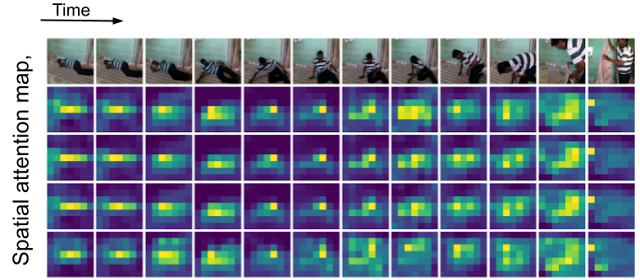
Visualization of the spatial attention maps in TokenLearner, over time. As the person is moving in the scene, TokenLearner pays attention to different spatial locations to tokenize.

Conclusion
While Vision Transformers serve as powerful models for computer vision, a large number of tokens and their associated computation amount have been a bottleneck for their application to larger images and longer videos. In this project, we illustrate that retaining such a large number of tokens and fully processing them over the entire set of layers is not necessary. Further, we demonstrate that by learning a module that extracts tokens adaptively based on the input image allows attaining even better performance while saving compute. The proposed TokenLearner was particularly effective in video representation learning tasks, which we confirmed with multiple public datasets. A preprint of our work as well as code are publicly available.

Acknowledgement
We thank our co-authors: AJ Piergiovanni, Mostafa Dehghani, and Anelia Angelova. We also thank the Robotics at Google team members for the motivating discussions.

Source: Google AI Blog


Making Better Future Predictions by Watching Unlabeled Videos

Machine learning (ML) agents are increasingly deployed in the real world to make decisions and assist people in their daily lives. Making reasonable predictions about the future at varying timescales is one of the most important capabilities for such agents because it enables them to predict changes in the world around them, including other agents’ behaviors, and plan how to act next. Importantly, successful future prediction requires both capturing meaningful transitions in the environment (e.g., dough transforming into bread) and adapting to how transitions unfold over time in order to make decisions.

Previous work in future prediction from visual observations has largely been constrained by the format of its output (e.g., pixels that represent an image) or a manually-defined set of human activities (e.g., predicting if someone will keep walking, sit down, or jump). These are either too detailed and hard to predict or lack important information about the richness of the real world. For example, predicting “person jumping” does not capture why they’re jumping, what they’re jumping onto, etc. Also, with very few exceptions, previous models were designed to make predictions at a fixed offset into the future, which is a limiting assumption because we rarely know when meaningful future states will happen.

For example, in a video about making ice cream (depicted below), the meaningful transition from “cream” to “ice cream” occurs over 35 seconds, so models predicting such transitions would need to look 35 seconds ahead. But this time interval varies a large amount across different activities and videos — meaningful transitions occur at any distance into the future. Learning to make such predictions at flexible intervals is hard because the desired ground truth may be relatively ambiguous. For example, the correct prediction could be the just-churned ice cream in the machine, or scoops of the ice cream in a bowl. In addition, collecting such annotations at scale (i.e., frame-by-frame for millions of videos) is infeasible. However, many existing instructional videos come with speech transcripts, which often offer concise, general descriptions throughout entire videos. This source of data can guide a model’s attention toward important parts of the video, obviating the need for manual labeling and allowing a flexible, data-driven definition of the future.

In “Learning Temporal Dynamics from Cycles in Narrated Video”, published at ICCV 2021, we propose an approach that is self-supervised, using a recent large unlabeled dataset of diverse human action. The resulting model operates at a high level of abstraction, can make predictions arbitrarily far into the future, and chooses how far into the future to predict based on context. Called Multi-Modal Cycle Consistency (MMCC), it leverages narrated instructional video to learn a strong predictive model of the future. We demonstrate how MMCC can be applied, without fine-tuning, to a variety of challenging tasks, and qualitatively examine its predictions. In the example below, MMCC predicts the future (d) from present frame (a), rather than less relevant potential futures (b) or (c).

This work uses cues from vision and language to predict high-level changes (such as cream becoming ice cream) in video (video from HowTo100M).

Viewing Videos as Graphs
The foundation of our method is to represent narrated videos as graphs. We view videos as a collection of nodes, where nodes are either video frames (sampled at 1 frame per second) or segments of narrated text (extracted with automatic speech recognition systems), encoded by neural networks. During training, MMCC constructs a graph from the nodes, using cross-modal edges to connect video frames and text segments that refer to the same state, and temporal edges to connect the present (e.g., strawberry-flavored cream) and the future (e.g., soft-serve ice cream). The temporal edges operate on both modalities equally — they can start from either a video frame, some text, or both, and can connect to a future (or past) state in either modality. MMCC achieves this by learning a latent representation shared by frames and text and then making predictions in this representation space.

Multi-modal Cycle Consistency
To learn the cross-modal and temporal edge functions without supervision, we apply the idea of cycle consistency. Here, cycle consistency refers to the construction of cycle graphs, in which the model constructs a series of edges from an initial node to other nodes and back again: Given a start node (e.g., a sample video frame), the model is expected to find its cross-modal counterpart (i.e., text describing the frame) and combine them as the present state. To do this, at the start of training, the model assumes that frames and text with the same timestamps are counterparts, but then relaxes this assumption later. The model then predicts a future state, and the node most similar to this prediction is selected. Finally, the model attempts to invert the above steps by predicting the present state backward from the future node, and thus connecting the future node back with the start node.

The discrepancy between the model’s prediction of the present from the future and the actual present is the cycle-consistency loss. Intuitively, this training objective requires the predicted future to contain enough information about its past to be invertible, leading to predictions that correspond to meaningful changes to the same entities (e.g., tomato becoming marinara sauce, or flour and eggs in a bowl becoming dough). Moreover, the inclusion of cross-modal edges ensures future predictions are meaningful in either modality.

To learn the temporal and cross-modal edge functions end-to-end, we use the soft attention technique, which first outputs how likely each node is to be the target node of the edge, and then “picks” a node by taking the weighted average among all possible candidates. Importantly, this cyclic graph constraint makes few assumptions for the kind of temporal edges the model should learn, as long as they end up forming a consistent cycle. This enables the emergence of long-term temporal dynamics critical for future prediction without requiring manual labels of meaningful changes.

An example of the training objective: A cycle graph is expected to be constructed between the chicken with soy sauce and the chicken in chili oil because they are two adjacent steps in the chicken’s preparation (video from HowTo100M).

Discovering Cycles in Real-World Video
MMCC is trained without any explicit ground truth, using only long video sequences and randomly sampled starting conditions (a frame or text excerpt) and asking the model to find temporal cycles. After training, MMCC can identify meaningful cycles that capture complex changes in video.

Given frames as input (left), MMCC selects relevant text from video narrations and uses both modalities to predict a future frame (middle). It then finds text relevant to this future and uses it to predict the past (right). Using its knowledge of how objects and scenes change over time, MMCC “closes the cycle” and ends up where it started (videos from HowTo100M).
The model can also start from narrated text rather than frames and still find relevant transitions (videos from HowTo100M).

Zero-Shot Applications
For MMCC to identify meaningful transitions over time in an entire video, we define a “likely transition score” for each pair (A, B) of frames in a video, according to the model's predictions — the closer B is to our model’s prediction of the future of A, the higher the score assigned. We then rank all pairs according to this score and show the highest-scoring pairs of present and future frames detected in previously unseen videos (examples below).

The highest-scoring pairs from eight random videos, which showcase the versatility of the model across a wide range of tasks (videos from HowTo100M).

We can use this same approach to temporally sort an unordered collection of video frames without any fine-tuning by finding an ordering that maximizes the overall confidence scores between all adjacent frames in the sorted sequence.

Left: Shuffled frames from three videos. Right: MMCC unshuffles the frames. The true order is shown under each frame. Even when MMCC does not predict the ground truth, its predictions often appear reasonable, and so, it can present an alternate ordering (videos from HowTo100M).

Evaluating Future Prediction
We evaluate the model’s ability to anticipate action, potentially minutes in advance, using the top-k recall metric, which here measures a model’s ability to retrieve the correct future (higher is better). On CrossTask, a dataset of instruction videos with labels describing key steps, MMCC outperforms the previous self-supervised state-of-the-art models in inferring possible future actions.

Recall
Model    Top-1       Top-5       Top-10   
Cross-modal    2.9 14.2 24.3
Repr. Ant. 3.0 13.3 26.0
MemDPC 2.9 15.8 27.4
TAP 4.5 17.1 27.9
MMCC 5.4 19.9 33.8

Conclusions
We have introduced a self-supervised method to learn temporal dynamics by cycling through narrated instructional videos. Despite the simplicity of the model’s architecture, it can discover meaningful long-term transitions in vision and language, and can be applied without further training to challenging downstream tasks, such as anticipating far-away action and ordering collections of images. An interesting future direction is transferring the model to agents so they can use it to conduct long-term planning.

Acknowledgements
The core team includes Dave Epstein, Jiajun Wu, Cordelia Schmid, and Chen Sun. We thank Alexei Efros, Mia Chiquier, and Shiry Ginosar for their feedback, and Allan Jabri for inspiration in figure design. Dave would like to thank Dídac Surís and Carl Vondrick for insightful early discussions on cycling through time in video.

Source: Google AI Blog