Tag Archives: Computer Vision

Updating Google Maps with Deep Learning and Street View


Every day, Google Maps provides useful directions, real-time traffic information and information on businesses to millions of people. In order to provide the best experience for our users, this information has to constantly mirror an ever-changing world. While Street View cars collect millions of images daily, it is impossible to manually analyze more than 80 billion high resolution images collected to date in order to find new, or updated, information for Google Maps. One of the goals of the Google’s Ground Truth team is to enable the automatic extraction of information from our geo-located imagery to improve Google Maps.

In “Attention-based Extraction of Structured Information from Street View Imagery”, we describe our approach to accurately read street names out of very challenging Street View images in many countries, automatically, using a deep neural network. Our algorithm achieves 84.2% accuracy on the challenging French Street Name Signs (FSNS) dataset, significantly outperforming the previous state-of-the-art systems. Importantly, our system is easily extensible to extract other types of information out of Street View images as well, and now helps us automatically extract business names from store fronts. We are excited to announce that this model is now publicly available!
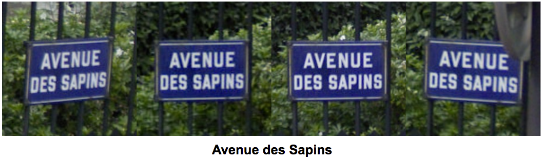
Example of street name from the FSNS dataset correctly transcribed by our system. Up to four views of the same sign are provided.
Text recognition in a natural environment is a challenging computer vision and machine learning problem. While traditional Optical Character Recognition (OCR) systems mainly focus on extracting text from scanned documents, text acquired from natural scenes is more challenging due to visual artifacts, such as distortion, occlusions, directional blur, cluttered background or different viewpoints. Our efforts to solve this research challenge first began in 2008, when we used neural networks to blur faces and license plates in Street View images to protect the privacy of our users. From this initial research, we realized that with enough labeled data, we could additionally use machine learning not only to protect the privacy of our users, but also to automatically improve Google Maps with relevant up-to-date information.

In 2014, Google’s Ground Truth team published a state-of-the-art method for reading street numbers on the Street View House Numbers (SVHN) dataset, implemented by then summer intern (now Googler) Ian Goodfellow. This work was not only of academic interest but was critical in making Google Maps more accurate. Today, over one-third of addresses globally have had their location improved thanks to this system. In some countries, such as Brazil, this algorithm has improved more than 90% of the addresses in Google Maps today, greatly improving the usability of our maps.

The next logical step was to extend these techniques to street names. To solve this problem, we created and released French Street Name Signs (FSNS), a large training dataset of more than 1 million street names. The FSNS dataset was a multi-year effort designed to allow anyone to improve their OCR models on a challenging and real use case. FSNS dataset is much larger and more challenging than SVHN in that accurate recognition of street signs may require combining information from many different images.
These are examples of challenging signs that are properly transcribed by our system by selecting or combining understanding across images. The second example is extremely challenging by itself, but the model learned a language model prior that enables it to remove ambiguity and correctly read the street name.
With this training set, Google intern Zbigniew Wojna spent the summer of 2016 developing a deep learning model architecture to automatically label new Street View imagery. One of the interesting strengths of our new model is that it can normalize the text to be consistent with our naming conventions, as well as ignore extraneous text, directly from the data itself.
Example of text normalization learned from data in Brazil. Here it changes “AV.” into “Avenida” and “Pres.” into “Presidente” which is what we desire.
In this example, the model is not confused from the fact that there is two street names, properly normalizes “Av” into “Avenue” as well as correctly ignores the number “1600”.
While this model is accurate, it did show a sequence error rate of 15.8%. However, after analyzing failure cases, we found that 48% of them were due to ground truth errors, highlighting the fact that this model is on par with the label quality (a full analysis our error rate can be found in our paper).

This new system, combined with the one extracting street numbers, allows us to create new addresses directly from imagery, where we previously didn’t know the name of the street, or the location of the addresses. Now, whenever a Street View car drives on a newly built road, our system can analyze the tens of thousands of images that would be captured, extract the street names and numbers, and properly create and locate the new addresses, automatically, on Google Maps.

But automatically creating addresses for Google Maps is not enough -- additionally we want to be able to provide navigation to businesses by name. In 2015, we published “Large Scale Business Discovery from Street View Imagery”, which proposed an approach to accurately detect business store-front signs in Street View images. However, once a store front is detected, one still needs to accurately extract its name for it to be useful -- the model must figure out which text is the business name, and which text is not relevant. We call this extracting “structured text” information out of imagery. It is not just text, it is text with semantic meaning attached to it.

Using different training data, the same model architecture that we used to read street names can also be used to accurately extract business names out of business facades. In this particular case, we are able to only extract the business name which enables us to verify if we already know about this business in Google Maps, allowing us to have more accurate and up-to-date business listings.
The system is correctly able to predict the business name ‘Zelina Pneus’, despite not receiving any data about the true location of the name in the image. Model is not confused by the tire brands that the sign indicates are available at the store.
Applying these large models across our more than 80 billion Street View images requires a lot of computing power. This is why the Ground Truth team was the first user of Google's TPUs, which were publicly announced earlier this year, to drastically reduce the computational cost of the inferences of our pipeline.

People rely on the accuracy of Google Maps in order to assist them. While keeping Google Maps up-to-date with the ever-changing landscape of cities, roads and businesses presents a technical challenge that is far from solved, it is the goal of the Ground Truth team to drive cutting-edge innovation in machine learning to create a better experience for over one billion Google Maps users.

PhotoScan: Taking Glare-Free Pictures of Pictures


Yesterday, we released an update to PhotoScan, an app for iOS and Android that allows you to digitize photo prints with just a smartphone. One of the key features of PhotoScan is the ability to remove glare from prints, which are often glossy and reflective, as are the plastic album pages or glass-covered picture frames that host them. To create this feature, we developed a unique blend of computer vision and image processing techniques that can carefully align and combine several slightly different pictures of a print to separate the glare from the image underneath.
Left: A regular digital picture of a physical print. Right: Glare-free digital output from PhotoScan
When taking a single picture of a photo, determining which regions of the picture are the actual photo and which regions are glare is challenging to do automatically. Moreover, the glare may often saturate regions in the picture, rendering it impossible to see or recover the parts of the photo underneath it. But if we take several pictures of the photo while moving the camera, the position of the glare tends to change, covering different regions of the photo. In most cases we found that every pixel of the photo is likely not to be covered by glare in at least one of the pictures. While no single view may be glare-free, we can combine multiple pictures of the printed photo taken at different angles to remove the glare. The challenge is that the images need to be aligned very accurately in order to combine them properly, and this processing needs to run very quickly on the phone to provide a near instant experience.
Left: The captured, input images (5 in total). Right: If we stabilize the images on the photo, we can see just the glare moving, covering different parts of the photo. Notice no single image is glare-free.
Our technique is inspired by our earlier work published at SIGGRAPH 2015, which we dubbed “obstruction-free photography”. It uses similar principles to remove various types of obstructions from the field of view. However, the algorithm we originally proposed was based on a generative model where the motion and appearance of both the main scene and the obstruction layer are estimated. While that model is quite powerful and can remove a variety of obstructions, it is too computationally expensive to be run on smartphones. We therefore developed a simpler model that treats glare as an outlier, and only attempts to register the underlying, glare-free photo. While this model is simpler, the task is still quite challenging as the registration needs to be highly accurate and robust.

How it Works
We start from a series of pictures of the print taken by the user while moving the camera. The first picture - the “reference frame” - defines the desired output viewpoint. The user is then instructed to take four additional frames. In each additional frame, we detect sparse feature points (we compute ORB features on Harris corners) and use them to establish homographies mapping each frame to the reference frame.
Left: Detected feature matches between the reference frame and each other frame (left), and the warped frames according to the estimated homographies (right).
While the technique may sound straightforward, there is a catch - homographies are only able to align flat images. But printed photos are often not entirely flat (as is the case with the example shown above). Therefore, we use optical flow — a fundamental, computer vision representation for motion, which establishes pixel-wise mapping between two images — to correct the non-planarities. We start from the homography-aligned frames, and compute “flow fields” to warp the images and further refine the registration. In the example below, notice how the corners of the photo on the left slightly “move” after registering the frames using only homographies. The right hand side shows how the photo is better aligned after refining the registration using optical flow.
Comparison between the warped frames using homographies (left) and after the additional warp refinement using optical flow (right).
The difference in the registration is subtle, but has a big impact on the end result. Notice how small misalignments manifest themselves as duplicated image structures in the result, and how these artifacts are alleviated with the additional flow refinement.
Comparison between the glare removal result with (right) and without (left) optical flow refinement. In the result using homographies only (left), notice artifacts around the eye, nose and teeth of the person, and duplicated stems and flower petals on the fabric.
Here too, the challenge was to make optical flow, a naturally slow algorithm, work very quickly on the phone. Instead of computing optical flow at each pixel as done traditionally (the number of flow vectors computed is equal to the number of input pixels), we represent a flow field by a smaller number of control points, and express the motion at each pixel in the image as a function of the motion at the control points. Specifically, we divide each image into tiled, non-overlapping cells to form a coarse grid, and represent the flow of a pixel in a cell as the bilinear combination of the flow at the four corners of the cell that contains it.

The grid setup for grid optical flow. A point p is represented as the bilinear interpolation of the four corner points of the cell that encapsulates it.
Left: Illustration of the computed flow field on one of the frames. Right: The flow color coding: orientation and magnitude represented by hue and saturation, respectively.
This results in a much smaller problem to solve, since the number of flow vectors to compute now equals the number of grid points, which is typically much smaller than the number of pixels. This process is similar in nature to the spline-based image registration described in Szeliski and Coughlan (1997). With this algorithm, we were able to reduce the optical flow computation time by a factor of ~40 on a Pixel phone!
Flipping between the homography-registered frame and the flow-refined warped frame (using the above flow field), superimposed on the (clean) reference frame, shows how the computed flow field “snaps” image parts to their corresponding parts in the reference frame, improving the registration.
Finally, in order to compose the glare-free output, for any given location in the registered frames, we examine the pixel values, and use a soft minimum algorithm to obtain the darkest observed value. More specifically, we compute the expectation of the minimum brightness over the registered frames, assigning less weight to pixels close to the (warped) image boundaries. We use this method rather than computing the minimum directly across the frames due to the fact that corresponding pixels at each frame may have slightly different brightness. Therefore, per-pixel minimum can produce visible seams due to sudden intensity changes at boundaries between overlaid images.
Regular minimum (left) versus soft minimum (right) over the registered frames.
The algorithm can support a variety of scanning conditions — matte and gloss prints, photos inside or outside albums, magazine covers.

Input     Registered     Glare-free
To get the final result, the Photos team has developed a method that automatically detects and crops the photo area, and rectifies it to a frontal view. Because of perspective distortion, the scanned rectangular photo usually appears to be a quadrangle on the image. The method analyzes image signals, like color and edges, to figure out the exact boundary of the original photo on the scanned image, then applies a geometric transformation to rectify the quadrangle area back to its original rectangular shape yielding high-quality, glare-free digital version of the photo.
So overall, quite a lot going on under the hood, and all done almost instantaneously on your phone! To give PhotoScan a try, download the app on Android or iOS.

Advancing Research on Video Understanding with the YouTube-BoundingBoxes Dataset


One of the most challenging research areas in machine learning today is enabling computers to understand what a scene is about. For example, while humans know that a ball that disappears behind a wall only to reappear a moment later is very likely the same object, this is not at all obvious to an algorithm. Understanding this requires not only a global picture of what objects are contained in each frame of a video, but also where those objects are located within the frame and their locations over time. Just last year we published YouTube-8M, a dataset consisting of automatically labelled YouTube videos. And while this helps further progress in the field, it is only one piece to the puzzle.

Today, in order to facilitate progress in video understanding research, we are introducing YouTube-BoundingBoxes, a dataset consisting of 5 million bounding boxes spanning 23 object categories, densely labeling segments from 210,000 YouTube videos. To date, this is the largest manually annotated video dataset containing bounding boxes, which track objects in temporally contiguous frames. The dataset is designed to be large enough to train large-scale models, and be representative of videos captured in natural settings. Importantly, the human-labelled annotations contain objects as they appear in the real world with partial occlusions, motion blur and natural lighting.
Summary of dataset statistics. Bar Chart: Relative number of detections in existing image (red) and video (blue) data sets. The YouTube BoundingBoxes dataset (YT-BB) is at the bottom, is at the bottom. Table: The three columns are counts for: classification annotations, bounding boxes, and unique videos with bounding boxes. Full details on the dataset can be found in the preprint.
A key feature of this dataset is that bounding box annotations are provided for entire video segments. These bounding box annotations may be used to train models that explicitly leverage this temporal information to identify, localize and track objects over time. In a video, individual annotated objects might become entirely occluded and later return in subsequent frames. These annotations of individual objects are sometimes not recognizable from individual frames, but can be understood and recognized in the context of the video if the objects are localized and tracked accurately.
Three video segments, sampled at 1 frame per second. The final frame of each example shows how it is visually challenging to recognize the bounded object, due to blur or occlusion (train example, blue arrow). However, temporally-related frames, where the object has been more clearly identified, can allow object classes to be inferred. Note how only visible parts are included in the box: the orange arrow in the bear example (middle row) points to the hidden head. The dog example illustrates tight bounding boxes that track the tail (orange arrows) and foot (blue arrows). The airplane example illustrates how partial objects are annotated (first frame) tracked across changes in perspective, occlusions and camera cuts.
We hope that this dataset might ultimately aid the computer vision and machine learning community and lead to new methods for analyzing and understanding real world vision problems. You can learn more about the dataset in this associated preprint.

Acknowledgements
The work was greatly helped along by Xin Pan and Thomas Silva, as well as support and advice from Manfred Georg, Sami Abu-El-Haija, Susanna Ricco and George Toderici.

Google Summer of Code 2016 wrap-up: CloudCV

This guest post is part of our ongoing series of posts from the students, mentors and organization administrators who participated in Google Summer of Code (GSoC), a program which gets university students contributing to open source software.

Google Summer of Code 2016 was a memorable one for CloudCV. Despite being a relatively “young” organization (this is just our second year as a mentor organization), there were many excellent applicants who put a tremendous amount of effort into their proposals and ramp-up tasks. It was difficult to choose!

CloudCV began in the summer of 2014 as a research project within the Machine Learning and Perception Lab at Virginia Tech, with the ambitious goal of democratizing computer vision and machine learning. We’re run exclusively by students and are working to enable developers, researchers, and fellow students to leverage artificial intelligence technology as a service and to share state of the art algorithms with the research community.

In line with this goal, we decided to build two tools that cater to computer vision researchers and hobbyists alike: CloudCV-fy your code and CloudCV-IDE. Though building two new platforms from the ground up was going to be challenging, our students’ motivation was overwhelming and their performance surpassed all expectations. We even demonstrated their work at CVPR 2016, a top-tier computer vision conference!

CloudCV-fy

A recurring use case for computer vision researchers, and many others, is to build a web-based demo and REST API to demonstrate the capabilities of their creations to the world. But web development involves writing hundred of lines of additional code across multiple languages (HTML, CSS, JavaScript, etc), which takes time away from research.


Our first student, Ashish Chaudhary, took on this problem by building CloudCV-fy. Over many iterations of design and development, Ashish delivered a tool that allows a user to simply write lightweight wrappers around their machine learning model/library and be done. CloudCV-fy automatically builds web-based interactive demos for them -- no need to tinker with HTML, CSS or JavaScript. Code to demo. Done.

The demo can be hosted on our servers, the user’s own server or any third party cloud service. As a result of this, researchers can focus on what they do best: designing and training models. CloudCV handles the rest. You can learn more in the write-up Ashish did on his blog.

CloudCV-IDE

There has been an explosion in the number of deep learning frameworks and it is difficult for researchers to keep up with all the latest tools. CloudCV-IDE, built by student Gaurav Gupta, addresses this by allowing a user to build a deep learning network with a drag-and-drop interface, then export to the deep learning framework of their choice (Caffe, TensorFlow, etc).

Gaurav also added support to import model configuration files in order to visualize any architecture. This is one of the first attempts to do this.


By the end of the summer, Gaurav delivered a great UI to visualize models with robust support for Caffe and TensorFlow back-ends. This was a successful start that we plan to build on by supporting more frameworks and facilitating collaborative building of deep learning models.

Overall, this was a highly productive GSoC for CloudCV. Our tools are under active development and we welcome contributions and ideas for new features.

We will definitely apply for GSoC 2017. If you are a student interested in participating we encourage you to get involved early! Feel free to reach out to us on our Gitter channel or on our mailing list.

By Viraj Prabhu, Organization Administrator for CloudCV

Get moving with the new Motion Stills


Last June, we released Motion Stills, an iOS app that uses our video stabilization technology to create easily shareable GIFs from Apple Live Photos. Since then, we integrated Motion Stills into Google Photos for iOS and thought of ways to improve it, taking into account your ideas for new features.

Today, we are happy to announce a major new update to the Motion Stills app that will help you create even more beautiful videos and fun GIFs using motion-tracked text overlays, super-resolution videos, and automatic cinemagraphs.

Motion Text

We’ve added motion text so you can create moving text effects, similar to what you might see in movies and TV shows, directly on your phone. With Motion Text, you can easily position text anywhere over your video to get the exact result you want. It only takes a second to initialize while you type, and a tracks at 1000 FPS throughout the whole Live Photo, so the process feels instantaneous.
To make this possible, we took the motion tracking technology that we run on YouTube servers for “Privacy Blur”, and made it run even faster on your device. How? We first create motion metadata for your video by leveraging machine learning to classify foreground/background features as well as to model temporally coherent camera motion. We then take this metadata, and use it as input to an algorithm that can track individual objects while discriminating it from others. The algorithm models each object’s state that includes its motion in space, an implicit appearance model (described as a set of its moving parts), and its centroid and extent, as shown in the figure below.
Enhance! your videos with better detail and loops

Last month, we published the details of our state-of-the-art RAISR technology, which employs machine learning to create super-resolution detail in images. This technology is now available in Motion Stills, automatically sharpening every video you export.

We are also going beyond stabilization to bring you fully automatic cinemagraphs. After freezing the background into a still photo, we analyze our result to optimize for the perfect loop transition. By considering a range of start and end frames, we build a matrix of transition scores between frame pairs. A significant minimum in this matrix reflects the perfect transition, resulting in an endless loop of motion stillness.
Continuing improve the experience

Thanks to your feedback, we’ve additionally rebuilt our navigation and added more tutorials. We’ve also added Apple’s 3D touch to let you “peek and pop” clips in your stream and movie tray. Lots more is coming to address your top requests, so please download the new release of Motion Stills and keep sending us feedback with #motionstills on your favorite social media.

Graph-powered Machine Learning at Google


Recently, there have been significant advances in Machine Learning that enable computer systems to solve complex real-world problems. One of those advances is Google’s large scale, graph-based machine learning platform, built by the Expander team in Google Research. A technology that is behind many of the Google products and features you may use everyday, graph-based machine learning is a powerful tool that can be used to power useful features such as reminders in Inbox and smart messaging in Allo, or used in conjunction with deep neural networks to power the latest image recognition system in Google Photos.
Learning with Minimal Supervision

Much of the recent success in deep learning and machine learning, in general, can be attributed to models that demonstrate high predictive capacity when trained on large amounts of labeled data -- often millions of training examples. This is commonly referred to as “supervised learning” since it requires supervision, in the form of labeled data, to train the machine learning systems. (Conversely, some machine learning methods operate directly on raw data without any supervision, a paradigm referred to as unsupervised learning.)

However, the more difficult the task, the harder it is to get sufficient high-quality labeled data. It is often prohibitively labor intensive and time-consuming to collect labeled data for every new problem. This motivated the Expander research team to build new technology for powering machine learning applications at scale and with minimal supervision.

Expander’s technology draws inspiration from how humans learn to generalize and bridge the gap between what they already know (labeled information) and novel, unfamiliar observations (unlabeled information). Known as “semi-supervised” learning, this powerful technique enables us to build systems that can work in situations where training data may be sparse. One of the key advantages to a graph-based semi-supervised machine learning approach is the fact that (a) one models labeled and unlabeled data jointly during learning, leveraging the underlying structure in the data, (b) one can easily combine multiple types of signals (for example, relational information from Knowledge Graph along with raw features) into a single graph representation and learn over them. This is in contrast to other machine learning approaches, such as neural network methods, in which it is typical to first train a system using labeled data with features and then apply the trained system to unlabeled data.

Graph Learning: How It Works

At its core, Expander’s platform combines semi-supervised machine learning with large-scale graph-based learning by building a multi-graph representation of the data with nodes corresponding to objects or concepts and edges connecting concepts that share similarities. The graph typically contains both labeled data (nodes associated with a known output category or label) and unlabeled data (nodes for which no labels were provided). Expander’s framework then performs semi-supervised learning to label all nodes jointly by propagating label information across the graph.

However, this is easier said than done! We have to (1) learn efficiently at scale with minimal supervision (i.e., tiny amount of labeled data), (2) operate over multi-modal data (i.e., heterogeneous representations and various sources of data), and (3) solve challenging prediction tasks (i.e., large, complex output spaces) involving high dimensional data that might be noisy.

One of the primary ingredients in the entire learning process is the graph and choice of connections. Graphs come in all sizes, shapes and can be combined from multiple sources. We have observed that it is often beneficial to learn over multi-graphs that combine information from multiple types of data representations (e.g., image pixels, object categories and chat response messages for PhotoReply in Allo). The Expander team’s graph learning platform automatically generates graphs directly from data based on the inferred or known relationships between data elements. The data can be structured (for example, relational data) or unstructured (for example, sparse or dense feature representations extracted from raw data).

To understand how Expander’s system learns, let us consider an example graph shown below.
There are two types of nodes in the graph: “grey” represents unlabeled data whereas the colored nodes represent labeled data. Relationships between node data is represented via edges and thickness of each edge indicates strength of the connection. We can formulate the semi-supervised learning problem on this toy graph as follows: predict a color (“red” or “blue”) for every node in the graph. Note that the specific choice of graph structure and colors depend on the task. For example, as shown in this research paper we recently published, a graph that we built for the Smart Reply feature in Inbox represents email messages as nodes and colors indicate semantic categories of user responses (e.g., “yes”, “awesome”, “funny”).

The Expander graph learning framework solves this labeling task by treating it as an optimization problem. At the simplest level, it learns a color label assignment for every node in the graph such that neighboring nodes are assigned similar colors depending on the strength of their connection. A naive way to solve this would be to try to learn a label assignment for all nodes at once -- this method does not scale to large graphs. Instead, we can optimize the problem formulation by propagating colors from labeled nodes to their neighbors, and then repeating the process. In each step, an unlabeled node is assigned a label by inspecting color assignments of its neighbors. We can update every node’s label in this manner and iterate until the whole graph is colored. This process is a far more efficient way to optimize the same problem and the sequence of iterations converges to a unique solution in this case. The solution at the end of the graph propagation looks something like this:
Semi-supervised learning on a graph
In practice, we use complex optimization functions defined over the graph structure, which incorporate additional information and constraints for semi-supervised graph learning that can lead to hard, non-convex problems. The real challenge, however, is to scale this efficiently to graphs containing billions of nodes, trillions of edges and for complex tasks involving billions of different label types.

To tackle this challenge, we created an approach outlined in Large Scale Distributed Semi-Supervised Learning Using Streaming Approximation, published last year. It introduces a streaming algorithm to process information propagated from neighboring nodes in a distributed manner that makes it work on very large graphs. In addition, it addresses other practical concerns, notably it guarantees that the space complexity or memory requirements of the system stays constant regardless of the difficulty of the task, i.e., the overall system uses the same amount of memory regardless of whether the number of prediction labels is two (as in the above toy example) or a million or even a billion. This enables wide-ranging applications for natural language understanding, machine perception, user modeling and even joint multimodal learning for tasks involving multiple modalities such as text, image and video inputs.

Language Graphs for Learning Humor

As an example use of graph-based machine learning, consider emotion labeling, a language understanding task in Smart Reply for Inbox, where the goal is to label words occurring in natural language text with their fine-grained emotion categories. A neural network model is first applied to a text corpus to learn word embeddings, i.e., a mathematical vector representation of the meaning of each word. The dense embedding vectors are then used to build a sparse graph where nodes correspond to words and edges represent semantic relationship between them. Edge strength is computed using similarity between embedding vectors — low similarity edges are ignored. We seed the graph with emotion labels known a priori for a few nodes (e.g., laugh is labeled as “funny”) and then apply semi-supervised learning over the graph to discover emotion categories for remaining words (e.g., ROTFL gets labeled as “funny” owing to its multi-hop semantic connection to the word “laugh”).
Learning emotion associations using graph constructed from word embedding vectors
For applications involving large datasets or dense representations that are observed (e.g., pixels from images) or learned using neural networks (e.g., embedding vectors), it is infeasible to compute pairwise similarity between all objects to construct edges in the graph. The Expander team solves this problem by leveraging approximate, linear-time graph construction algorithms.

Graph-based Machine Intelligence in Action

The Expander team’s machine learning system is now being used on massive graphs (containing billions of nodes and trillions of edges) to recognize and understand concepts in natural language, images, videos, and queries, powering Google products for applications like reminders, question answering, language translation, visual object recognition, dialogue understanding, and more.

We are excited that with the recent release of Allo, millions of chat users are now experiencing smart messaging technology powered by the Expander team’s system for understanding and assisting with chat conversations in multiple languages. Also, this technology isn’t used only for large-scale models in the cloud - as announced this past week, Android Wear has opened up an on-device Smart Reply capability for developers that will provide smart replies for any messaging application. We’re excited to tackle even more challenging Internet-scale problems with Expander in the years to come.

Acknowledgements

We wish to acknowledge the hard work of all the researchers, engineers, product managers, and leaders across Google who helped make this technology a success. In particular, we would like to highlight the efforts of Allan Heydon, Andrei Broder, Andrew Tomkins, Ariel Fuxman, Bo Pang, Dana Movshovitz-Attias, Fritz Obermeyer, Krishnamurthy Viswanathan, Patrick McGregor, Peter Young, Robin Dua, Sujith Ravi and Vivek Ramavajjala.

Introducing the Open Images Dataset

Originally posted on the Google Research Blog

In the last few years, advances in machine learning have enabled Computer Vision to progress rapidly, allowing for systems that can automatically caption images to apps that can create natural language replies in response to shared photos. Much of this progress can be attributed to publicly available image datasets, such as ImageNet and COCO for supervised learning, and YFCC100M for unsupervised learning.

Today, we introduce Open Images, a dataset consisting of ~9 million URLs to images that have been annotated with labels spanning over 6000 categories. We tried to make the dataset as practical as possible: the labels cover more real-life entities than the 1000 ImageNet classes, there are enough images to train a deep neural network from scratch and the images are listed as having a Creative Commons Attribution license*.

The image-level annotations have been populated automatically with a vision model similar to Google Cloud Vision API. For the validation set, we had human raters verify these automated labels to find and remove false positives. On average, each image has about 8 labels assigned. Here are some examples:
Annotated images form the Open Images dataset. Left: Ghost Arches by Kevin Krejci. Right: Some Silverware by J B. Both images used under CC BY 2.0 license
We have trained an Inception v3 model based on Open Images annotations alone, and the model is good enough to be used for fine-tuning applications as well as for other things, like DeepDream or artistic style transfer which require a well developed hierarchy of filters. We hope to improve the quality of the annotations in Open Images the coming months, and therefore the quality of models which can be trained.

The dataset is a product of a collaboration between Google, CMU and Cornell universities, and there are a number of research papers built on top of the Open Images dataset in the works. It is our hope that datasets like Open Images and the recently released YouTube-8M will be useful tools for the machine learning community.

By Ivan Krasin and Tom Duerig, Software Engineers

* While we tried to identify images that are licensed under a Creative Commons Attribution license, we make no representations or warranties regarding the license status of each image and you should verify the license for each image yourself.

Introducing the Open Images Dataset


In the last few years, advances in machine learning have enabled Computer Vision to progress rapidly, allowing for systems that can automatically caption images to apps that can create natural language replies in response to shared photos. Much of this progress can be attributed to publicly available image datasets, such as ImageNet and COCO for supervised learning, and YFCC100M for unsupervised learning.

Today, we introduce Open Images, a dataset consisting of ~9 million URLs to images that have been annotated with labels spanning over 6000 categories. We tried to make the dataset as practical as possible: the labels cover more real-life entities than the 1000 ImageNet classes, there are enough images to train a deep neural network from scratch and the images are listed as having a Creative Commons Attribution license*.

The image-level annotations have been populated automatically with a vision model similar to Google Cloud Vision API. For the validation set, we had human raters verify these automated labels to find and remove false positives. On average, each image has about 8 labels assigned. Here are some examples:
Annotated images form the Open Images dataset. Left: Ghost Arches by Kevin Krejci. Right: Some Silverware by J B. Both images used under CC BY 2.0 license
We have trained an Inception v3 model based on Open Images annotations alone, and the model is good enough to be used for fine-tuning applications as well as for other things, like DeepDream or artistic style transfer which require a well developed hierarchy of filters. We hope to improve the quality of the annotations in Open Images the coming months, and therefore the quality of models which can be trained.

The dataset is a product of a collaboration between Google, CMU and Cornell universities, and there are a number of research papers built on top of the Open Images dataset in the works. It is our hope that datasets like Open Images and the recently released YouTube-8M will be useful tools for the machine learning community.


* While we tried to identify images that are licensed under a Creative Commons Attribution license, we make no representations or warranties regarding the license status of each image and you should verify the license for each image yourself.

Show and Tell: image captioning open sourced in TensorFlow


In 2014, research scientists on the Google Brain team trained a machine learning system to automatically produce captions that accurately describe images. Further development of that system led to its success in the Microsoft COCO 2015 image captioning challenge, a competition to compare the best algorithms for computing accurate image captions, where it tied for first place.

Today, we’re making the latest version of our image captioning system available as an open source model in TensorFlow. This release contains significant improvements to the computer vision component of the captioning system, is much faster to train, and produces more detailed and accurate descriptions compared to the original system. These improvements are outlined and analyzed in the paper Show and Tell: Lessons learned from the 2015 MSCOCO Image Captioning Challenge, published in IEEE Transactions on Pattern Analysis and Machine Intelligence.
Automatically captioned by our system.
So what’s new?

Our 2014 system used the Inception V1 image classification model to initialize the image encoder, which produces the encodings that are useful for recognizing different objects in the images. This was the best image model available at the time, achieving 89.6% top-5 accuracy on the benchmark ImageNet 2012 image classification task. We replaced this in 2015 with the newer Inception V2 image classification model, which achieves 91.8% accuracy on the same task. The improved vision component gave our captioning system an accuracy boost of 2 points in the BLEU-4 metric (which is commonly used in machine translation to evaluate the quality of generated sentences) and was an important factor of its success in the captioning challenge.

Today’s code release initializes the image encoder using the Inception V3 model, which achieves 93.9% accuracy on the ImageNet classification task. Initializing the image encoder with a better vision model gives the image captioning system a better ability to recognize different objects in the images, allowing it to generate more detailed and accurate descriptions. This gives an additional 2 points of improvement in the BLEU-4 metric over the system used in the captioning challenge.

Another key improvement to the vision component comes from fine-tuning the image model. This step addresses the problem that the image encoder is initialized by a model trained to classify objects in images, whereas the goal of the captioning system is to describe the objects in images using the encodings produced by the image model. For example, an image classification model will tell you that a dog, grass and a frisbee are in the image, but a natural description should also tell you the color of the grass and how the dog relates to the frisbee.

In the fine-tuning phase, the captioning system is improved by jointly training its vision and language components on human generated captions. This allows the captioning system to transfer information from the image that is specifically useful for generating descriptive captions, but which was not necessary for classifying objects. In particular, after fine-tuning it becomes better at correctly describing the colors of objects. Importantly, the fine-tuning phase must occur after the language component has already learned to generate captions - otherwise, the noisiness of the randomly initialized language component causes irreversible corruption to the vision component. For more details, read the full paper here.
Left: the better image model allows the captioning model to generate more detailed and accurate descriptions. Right: after fine-tuning the image model, the image captioning system is more likely to describe the colors of objects correctly.
Until recently our image captioning system was implemented in the DistBelief software framework. The TensorFlow implementation released today achieves the same level of accuracy with significantly faster performance: time per training step is just 0.7 seconds in TensorFlow compared to 3 seconds in DistBelief on an Nvidia K20 GPU, meaning that total training time is just 25% of the time previously required.

A natural question is whether our captioning system can generate novel descriptions of previously unseen contexts and interactions. The system is trained by showing it hundreds of thousands of images that were captioned manually by humans, and it often re-uses human captions when presented with scenes similar to what it’s seen before.
When the model is presented with scenes similar to what it’s seen before, it will often re-use human generated captions.
So does it really understand the objects and their interactions in each image? Or does it always regurgitate descriptions from the training data? Excitingly, our model does indeed develop the ability to generate accurate new captions when presented with completely new scenes, indicating a deeper understanding of the objects and context in the images. Moreover, it learns how to express that knowledge in natural-sounding English phrases despite receiving no additional language training other than reading the human captions.
Our model generates a completely new caption using concepts learned from similar scenes in the training set.
We hope that sharing this model in TensorFlow will help push forward image captioning research and applications, and will also allow interested people to learn and have fun. To get started training your own image captioning system, and for more details on the neural network architecture, navigate to the model’s home-page here. While our system uses the Inception V3 image classification model, you could even try training our system with the recently released Inception-ResNet-v2 model to see if it can do even better!

Improving Inception and Image Classification in TensorFlow


Earlier this week, we announced the latest release of the TF-Slim library for TensorFlow, a lightweight package for defining, training and evaluating models, as well as checkpoints and model definitions for several competitive networks in the field of image classification.

In order to spur even further progress in the field, today we are happy to announce the release of Inception-ResNet-v2, a convolutional neural network (CNN) that achieves a new state of the art in terms of accuracy on the ILSVRC image classification benchmark. Inception-ResNet-v2 is a variation of our earlier Inception V3 model which borrows some ideas from Microsoft's ResNet papers [1][2]. The full details of the model are in our arXiv preprint Inception-v4, Inception-ResNet and the Impact of Residual Connections on Learning.

Residual connections allow shortcuts in the model and have allowed researchers to successfully train even deeper neural networks, which have lead to even better performance. This has also enabled significant simplification of the Inception blocks. Just compare the model architectures in the figures below:
Schematic diagram of Inception V3
Schematic diagram of Inception-ResNet-v2
At the top of the second Inception-ResNet-v2 figure, you'll see the full network expanded. Notice that this network is considerably deeper than the previous Inception V3. Below in the main figure is an easier to read version of the same network where the repeated residual blocks have been compressed. Here, notice that the inception blocks have been simplified, containing fewer parallel towers than the previous Inception V3.

The Inception-ResNet-v2 architecture is more accurate than previous state of the art models, as shown in the table below, which reports the Top-1 and Top-5 validation accuracies on the ILSVRC 2012 image classification benchmark based on a single crop of the image. Furthermore, this new model only requires roughly twice the memory and computation compared to Inception V3.


Model
Architecture

Checkpoint

Top-1 Accuracy

Top-5 Accuracy

Code
80.4
95.3

Code
78.0
93.9

Code
76.8
93.2

Code
TBA
79.9*
95.2*
(*): Results quoted in ResNet paper.

As an example, while both Inception V3 and Inception-ResNet-v2 models excel at identifying individual dog breeds, the new model does noticeably better. For instance, whereas the old model mistakenly reported Alaskan Malamute for the picture on the right, the new Inception-ResNet-v2 model correctly identifies the dog breeds in both images.
An Alaskan Malamute (left) and a Siberian Husky (right). Images from Wikipedia
In order to allow people to immediately begin experimenting, we are also releasing a pre-trained instance of the new Inception-ResNet-v2, as part of the TF-Slim Image Model Library.

We are excited to see what the community does with this improved model, following along as people adapt it and compare its performance on various tasks. Want to get started? See the accompanying instructions on how to train, evaluate or fine-tune a network.

As always, releasing the code was a team effort. Specific thanks are due to:
  • Model Architecture - Christian Szegedy, Sergey Ioffe, Vincent Vanhoucke, Alex Alemi
  • Systems Infrastructure - Jon Shlens, Benoit Steiner, Mark Sandler, and David Andersen
  • TensorFlow-Slim - Sergio Guadarrama and Nathan Silberman
  • Model Visualization - Fernanda Viégas and James Wexler