Eric Christiansen, Senior Software Engineer, Google Research

In the fields of biology and medicine, microscopy allows researchers to observe details of cells and molecules which are unavailable to the naked eye. Transmitted light microscopy, where a biological sample is illuminated on one side and imaged, is relatively simple and well-tolerated by living cultures but produces images which can be difficult to properly assess. Fluorescence microscopy, in which biological objects of interest (such as cell nuclei) are specifically targeted with fluorescent molecules, simplifies analysis but requires complex sample preparation. With the increasing application of machine learning to the field of microscopy, including algorithms used to automatically assess the quality of images and assist pathologists diagnosing cancerous tissue, we wondered if we could develop a deep learning system that could combine the benefits of both microscopy techniques while minimizing the downsides.

With “In Silico Labeling: Predicting Fluorescent Labels in Unlabeled Images”, appearing today in Cell, we show that a deep neural network can predict fluorescence images from transmitted light images, generating labeled, useful, images without modifying cells and potentially enabling longitudinal studies in unmodified cells, minimally invasive cell screening for cell therapies, and investigations using large numbers of simultaneous labels. We also open sourced our network, along with the complete training and test data, a trained model checkpoint, and example code.

Background
Transmitted light microscopy techniques are easy to use, but can produce images in which it can be hard to tell what’s going on. An example is the following image from a phase-contrast microscope, in which the intensity of a pixel indicates the degree to which light was phase-shifted as it passed through the sample.

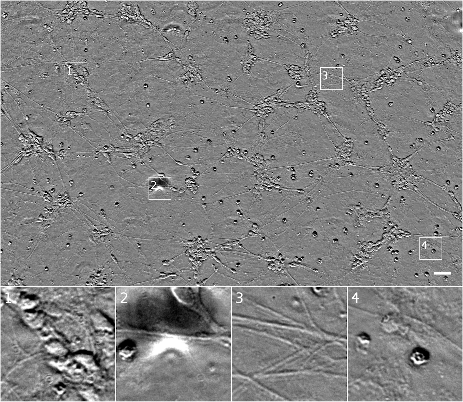
Transmitted light (phase-contrast) image of a human motor neuron culture derived from induced pluripotent stem cells. Outset 1 shows a cluster of cells, possibly neurons. Outset 2 shows a flaw in the image obscuring underlying cells. Outset 3 shows neurites. Outset 4 shows what appear to be dead cells. Scale bar is 40 μm. Source images for this and the following figures come from the Finkbeiner lab at the Gladstone Institutes.

In the above figure, it’s difficult to tell how many cells are in the cluster in Outset 1, or the locations and states of the cells in Outset 4 (hint: there’s a barely-visible flat cell in the upper-middle). It’s also difficult to get fine structures consistently in focus, such as the neurites in Outset 3.

We can get more information out of transmitted light microscopy by acquiring images in z-stacks: sets of images registered in (x, y) where z (the distance from the camera) is systematically varied. This causes different parts of the cells to come in and out of focus, which provides information about a sample’s 3D structure. Unfortunately, it often takes a trained eye to make sense of the z-stack, and analysis of such z-stacks has largely defied automation. An example z-stack is shown below.

A phase-contrast z-stack of the same cells. Note how the appearance changes as the focus is shifted. Now we can see that the fuzzy shape in the lower right of Outset 1 is a single oblong cell, and that the rightmost cell in Outset 4 is taller than the uppermost cell, possibly indicating that it has undergone programmed cell death.

In contrast, fluorescence microscopy images are easier to analyze, because samples are prepared with carefully engineered fluorescent labels which light up just what the researchers want to see. For example, most human cells have exactly one nucleus, so a nuclear label (such as the blue one below) makes it possible for simple tools to find and count cells in an image.

Fluorescence microscopy image of the same cells. The blue fluorescent label localizes to DNA, highlighting cell nuclei. The green fluorescent label localizes to a protein found only in dendrites, a neural substructure. The red fluorescent label localizes to a protein found only in axons, another neural substructure. With these labels it is much easier to understand what’s happening in the sample. For example, the green and red labels in Outset 1 confirm this is a neural cluster. The red label in Outset 3 shows that the neurites are axons, not dendrites. The upper-left blue dot in Outset 4 reveals a previously hard-to-see nucleus, and the lack of a blue dot for the cell at the left shows it to be DNA-free cellular debris.

However, fluorescence microscopy can have significant downsides. First, there is the complexity and variability introduced by the sample preparation and fluorescent labels themselves. Second, when there are many different fluorescent labels in a sample, spectral overlap can make it hard to tell which color belongs to which label, typically limiting researchers to three or four simultaneous labels in a sample. Third, fluorescence labeling may be toxic to cells and sometimes involves protocols that outright kill them, which makes labeling difficult to use in longitudinal studies where the same cells are followed through time.

Seeing more with deep learning
In our paper, we show that a deep neural network can predict fluorescence images from transmitted light z-stacks. To do this, we created a dataset of transmitted light z-stacks matched to fluorescence images and trained a neural network to predict the fluorescence images from the z-stacks. The following diagram explains the process.

Overview of our system. (A) The dataset of training examples: pairs of transmitted light images from z-stacks with pixel-registered sets of fluorescence images of the same scene. Several different fluorescent labels were used to generate fluorescence images and were varied between training examples; the checkerboard images indicate fluorescent labels which were not acquired for a given example. (B) The untrained deep network was (C) trained on the data A. (D) A z-stack of images of a novel scene. (E) The trained network, C, is used to predict fluorescence labels learned from A for each pixel in the novel images, D.

In the course of this work we developed a new neural network composed of three kinds of basic building-blocks, inspired by the modular design of Inception: an in-scale configuration which does not change the spatial scaling of the features, a down-scale configuration which doubles the spatial scaling, and an up-scale configuration which halves it. This lets us break the hard problem of network architecture design into two easier problems: the arrangement of the building-blocks (macro-architecture), and the design of the building-blocks themselves (micro-architecture). We solved the first problem using design principles discussed in the paper, and the second via an automated search powered by Google Hypertune.

To make sure our method was sound, we validated our model using data from an Alphabet lab as well as two external partners: Steve Finkbeiner's lab at the Gladstone Institutes, and the Rubin Lab at Harvard. These data spanned three transmitted light imaging modalities (bright-field, phase-contrast, and differential interference contrast) and three culture types (human motor neurons derived from induced pluripotent stem cells, rat cortical cultures, and human breast cancer cells). We found that our method can accurately predict several labels including those for nuclei, cell type (e.g. neural), and cell state (e.g. cell death). The following figure shows the model’s predictions alongside the transmitted light input and fluorescence ground-truth for our motor neuron example.

Animation showing the same cells in transmitted light and fluorescence imaging, along with predicted fluorescence labels from our model. Outset 2 shows the model predicts the correct labels despite the artifact in the input image. Outset 3 shows the model infers these processes are axons, possibly because of their distance from the nearest cells. Outset 4 shows the model sees the hard-to-see cell at the top, and correctly identifies the object at the left as DNA-free cell debris.

Try it for yourself!
We’ve open sourced our model, along with our full dataset, code for training and inference, and an example. We’re pleased to report that new labels can be learned with minimal additional training data: in the paper and example code, we show a new label may be learned from a single image. This is due to a phenomenon called transfer learning, where a model can learn a new task more quickly and using less training data if it has already mastered similar tasks.

We hope the ability to generate labeled, useful, images without modifying cells will open up completely new kinds of experiments in biology and medicine. If you’re excited to try this technology in your own work, please read the paper or check out the code!

Acknowledgements
We thank the Google Accelerated Science team for originating and developing this project and its publication, and additionally Kevin P. Murphy for supporting its publication. We thank Mike Ando, Youness Bennani, Amy Chung-Yu Chou, Jason Freidenfelds, Jason Miller, Kevin P. Murphy, Philip Nelson, Patrick Riley, and Samuel Yang for ideas and editing help with this post. This study was supported by NINDS (NS091046, NS083390, NS101995), the NIH’s National Institute on Aging (AG065151, AG058476), the NIH’s National Human Genome Research Institute (HG008105), Google, the ALS Association, and the Michael J. Fox Foundation.

References

1. MobileNets: Efficient Convolutional Neural Networks for Mobile Vision Applications, Howard AG, Zhu M, Chen B, Kalenichenko D, Wang W, Weyand T, Andreetto M, Adam H, arXiv:1704.04861, 2017.
2. MobileNetV2: Inverted Residuals and Linear Bottlenecks, Sandler M, Howard A, Zhu M, Zhmoginov A, Chen LC. arXiv preprint. arXiv:1801.04381, 2018.
3. Rethinking Atrous Convolution for Semantic Image Segmentation, Chen LC, Papandreou G, Schroff F, Adam H. arXiv:1706.05587, 2017.
4. Speed/accuracy trade-offs for modern convolutional object detectors, Huang J, Rathod V, Sun C, Zhu M, Korattikara A, Fathi A, Fischer I, Wojna Z, Song Y, Guadarrama S, Murphy K, CVPR 2017.
5. Deep Residual Learning for Image Recognition, He, Kaiming, Xiangyu Zhang, Shaoqing Ren, and Jian Sun. arXiv:1512.03385,2015
1 The shortcut (also known as skip) connections, popularized by ResNets[5] are commonly used to connect the non-bottleneck layers. MobilenNetV2 inverts this notion and connects the bottlenecks directly.
MobileNetV2: The Next Generation of On-Device Computer Vision Networks
Last year we introduced MobileNetV1, a family of general purpose computer vision neural networks designed with mobile devices in mind to support classification, detection and more. The ability to run deep networks on personal mobile devices improves user experience, offering anytime, anywhere access, with additional benefits for security, privacy, and energy consumption. As new applications emerge allowing users to interact with the real world in real time, so does the need for ever more efficient neural networks.
Today, we are pleased to announce the availability of MobileNetV2 to power the next generation of mobile vision applications. MobileNetV2 is a significant improvement over MobileNetV1 and pushes the state of the art for mobile visual recognition including classification, object detection and semantic segmentation. MobileNetV2 is released as part of TensorFlow-Slim Image Classification Library, or you can start exploring MobileNetV2 right away in Colaboratory. Alternately, you can download the notebook and explore it locally using Jupyter. MobileNetV2 is also available as modules on TF-Hub, and pretrained checkpoints can be found on github.
MobileNetV2 builds upon the ideas from MobileNetV1 [1], using depthwise separable convolution as efficient building blocks. However, V2 introduces two new features to the architecture: 1) linear bottlenecks between the layers, and 2) shortcut connections between the bottlenecks1. The basic structure is shown below.
Overview of MobileNetV2 Architecture. Blue blocks represent composite convolutional building blocks as shown above.
The intuition is that the bottlenecks encode the model’s intermediate inputs and outputs while the inner layer encapsulates the model’s ability to transform from lower-level concepts such as pixels to higher level descriptors such as image categories. Finally, as with traditional residual connections, shortcuts enable faster training and better accuracy. You can learn more about the technical details in our paper, “MobileNet V2: Inverted Residuals and Linear Bottlenecks”.
How does it compare to the first generation of MobileNets?
Overall, the MobileNetV2 models are faster for the same accuracy across the entire latency spectrum. In particular, the new models use 2x fewer operations, need 30% fewer parameters and are about 30-40% faster on a Google Pixel phone than MobileNetV1 models, all while achieving higher accuracy.
MobileNetV2 improves speed (reduced latency) and increased ImageNet Top 1 accuracy
MobileNetV2 is a very effective feature extractor for object detection and segmentation. For example, for detection when paired with the newly introduced SSDLite [2] the new model is about 35% faster with the same accuracy than MobileNetV1. We have open sourced the model under the Tensorflow Object Detection API [4].
Model
Params
Multiply-Adds
mAP
Mobile CPU
MobileNetV1 + SSDLite
5.1M
1.3B
22.2%
270ms
4.3M
0.8B
22.1%
200ms
To enable on-device semantic segmentation, we employ MobileNetV2 as a feature extractor in a reduced form of DeepLabv3 [3], that was announced recently. On the semantic segmentation benchmark, PASCAL VOC 2012, our resulting model attains a similar performance as employing MobileNetV1 as feature extractor, but requires 5.3 times fewer parameters and 5.2 times fewer operations in terms of Multiply-Adds.
mIOU
MobileNetV1 + DeepLabV3
11.15M
14.25B
75.29%
2.11M
2.75B
75.32%
As we have seen MobileNetV2 provides a very efficient mobile-oriented model that can be used as a base for many visual recognition tasks. We hope by sharing it with the broader academic and open-source community we can help to advance research and application development.
Source: Google AI Blog
Behind the Motion Photos Technology in Pixel 2
One of the most compelling things about smartphones today is the ability to capture a moment on the fly. With motion photos, a new camera feature available on the Pixel 2 and Pixel 2 XL phones, you no longer have to choose between a photo and a video so every photo you take captures more of the moment. When you take a photo with motion enabled, your phone also records and trims up to 3 seconds of video. Using advanced stabilization built upon technology we pioneered in Motion Stills for Android, these pictures come to life in Google Photos. Let’s take a look behind the technology that makes this possible!
Motion photos on the Pixel 2 in Google Photos. With the camera frozen in place the focus is put directly on the subjects. For more examples, check out this Google Photos album.
Camera Motion Estimation by Combining Hardware and Software
The image and video pair that is captured every time you hit the shutter button is a full resolution JPEG with an embedded 3 second video clip. On the Pixel 2, the video portion also contains motion metadata that is derived from the gyroscope and optical image stabilization (OIS) sensors to aid the trimming and stabilization of the motion photo. By combining software based visual tracking with the motion metadata from the hardware sensors, we built a new hybrid motion estimation for motion photos on the Pixel 2.
Our approach aligns the background more precisely than the technique used in Motion Stills or the purely hardware sensor based approach. Based on Fused Video Stabilization technology, it reduces the artifacts from the visual analysis due to a complex scene with many depth layers or when a foreground object occupies a large portion of the field of view. It also improves the hardware sensor based approach by refining the motion estimation to be more accurate, especially at close distances.
Motion photo as captured (left) and after freezing the camera by combining hardware and software For more comparisons, check out this Google Photos album.
The purely software-based technique we introduced in Motion Stills uses the visual data from the video frames, detecting and tracking features over consecutive frames yielding motion vectors. It then classifies the motion vectors into foreground and background using motion models such as an affine transformation or a homography. However, this classification is not perfect and can be misled, e.g. by a complex scene or dominant foreground.
Feature classification into background (green) and foreground (orange) by using the motion metadata from the hardware sensors of the Pixel 2. Notice how the new approach not only labels the skateboarder accurately as foreground but also the half-pipe that is at roughly the same depth.
For motion photos on Pixel 2 we improved this classification by using the motion metadata derived from the gyroscope and the OIS. This accurately captures the camera motion with respect to the scene at infinity, which one can think of as the background in the distance. However, for pictures taken at closer range, parallax is introduced for scene elements at different depth layers, which is not accounted for by the gyroscope and OIS. Specifically, we mark motion vectors that deviate too much from the motion metadata as foreground. This results in a significantly more accurate classification of foreground and background, which also enables us to use a more complex motion model known as mixture homographies that can account for rolling shutter and undo the distortions it causes.
Background motion estimation in motion photos. By using the motion metadata from Gyro and OIS we are able to accurately classify features from the visual analysis into foreground and background.
Motion Photo Stabilization and Playback
Once we have accurately estimated the background motion for the video, we determine an optimally stable camera path to align the background using linear programming techniques outlined in our earlier posts. Further, we automatically trim the video to remove any accidental motion caused by putting the phone away. All of this processing happens on your phone and produces a small amount of metadata per frame that is used to render the stabilized video in real-time using a GPU shader when you tap the Motion button in Google Photos. In addition, we play the video starting at the exact timestamp as the HDR+ photo, producing a seamless transition from still image to video.
Motion photos stabilize even complex scenes with large foreground motions.
Motion Photo Sharing
Using Google Photos, you can share motion photos with your friends and as videos and GIFs, watch them on the web, or view them on any phone. This is another example of combining hardware, software and Machine Learning to create new features for Pixel 2.
1. Encoder-Decoder with Atrous Separable Convolution for Semantic Image Segmentation, Liang-Chieh Chen, Yukun Zhu, George Papandreou, Florian Schroff, and Hartwig Adam, arXiv: 1802.02611, 2018.
2. Xception: Deep Learning with Depthwise Separable Convolutions, François Chollet, Proc. of CVPR, 2017.
3. Deformable Convolutional Networks — COCO Detection and Segmentation Challenge 2017 Entry, Haozhi Qi, Zheng Zhang, Bin Xiao, Han Hu, Bowen Cheng, Yichen Wei, and Jifeng Dai, ICCV COCO Challenge Workshop, 2017.
4. Semantic Image Segmentation with Deep Convolutional Nets and Fully Connected CRFs, Liang-Chieh Chen, George Papandreou, Iasonas Kokkinos, Kevin Murphy, and Alan L. Yuille, Proc. of ICLR, 2015.
5. Deeplab: Semantic Image Segmentation with Deep Convolutional Nets, Atrous Convolution, and Fully Connected CRFs, Liang-Chieh Chen, George Papandreou, Iasonas Kokkinos, Kevin Murphy, and Alan L. Yuille, TPAMI, 2017.
6. Rethinking Atrous Convolution for Semantic Image Segmentation, Liang-Chieh Chen, George Papandreou, Florian Schroff, and Hartwig Adam, arXiv:1706.05587, 2017.
Semantic Image Segmentation with DeepLab in TensorFlow
Semantic image segmentation, the task of assigning a semantic label, such as “road”, “sky”, “person”, “dog”, to every pixel in an image enables numerous new applications, such as the synthetic shallow depth-of-field effect shipped in the portrait mode of the Pixel 2 and Pixel 2 XL smartphones and mobile real-time video segmentation. Assigning these semantic labels requires pinpointing the outline of objects, and thus imposes much stricter localization accuracy requirements than other visual entity recognition tasks such as image-level classification or bounding box-level detection.
Today, we are excited to announce the open source release of our latest and best performing semantic image segmentation model, DeepLab-v3+ [1]*, implemented in TensorFlow. This release includes DeepLab-v3+ models built on top of a powerful convolutional neural network (CNN) backbone architecture [2, 3] for the most accurate results, intended for server-side deployment. As part of this release, we are additionally sharing our TensorFlow model training and evaluation code, as well as models already pre-trained on the Pascal VOC 2012 and Cityscapes benchmark semantic segmentation tasks.
Since the first incarnation of our DeepLab model [4] three years ago, improved CNN feature extractors, better object scale modeling, careful assimilation of contextual information, improved training procedures, and increasingly powerful hardware and software have led to improvements with DeepLab-v2 [5] and DeepLab-v3 [6]. With DeepLab-v3+, we extend DeepLab-v3 by adding a simple yet effective decoder module to refine the segmentation results especially along object boundaries. We further apply the depthwise separable convolution to both atrous spatial pyramid pooling [5, 6] and decoder modules, resulting in a faster and stronger encoder-decoder network for semantic segmentation.
Modern semantic image segmentation systems built on top of convolutional neural networks (CNNs) have reached accuracy levels that were hard to imagine even five years ago, thanks to advances in methods, hardware, and datasets. We hope that publicly sharing our system with the community will make it easier for other groups in academia and industry to reproduce and further improve upon state-of-art systems, train models on new datasets, and envision new applications for this technology.
* DeepLab-v3+ is not used to power Pixel 2's portrait mode or real time video segmentation. These are mentioned in the post as examples of features this type of technology can enable.
Introducing the iNaturalist 2018 Challenge
Thanks to recent advances in deep learning, the visual recognition abilities of machines have improved dramatically, permitting the practical application of computer vision to tasks ranging from pedestrian detection for self-driving cars to expression recognition in virtual reality. One area that remains challenging for computers, however, is fine-grained and instance-level recognition. Earlier this month, we posted an instance-level landmark recognition challenge for identifying individual landmarks. Here we focus on fine-grained visual recognition, which is to distinguish species of animals and plants, car and motorcycle models, architectural styles, etc. For computers, discriminating fine-grained categories is challenging because many categories have relatively few training examples (i.e., the long tail problem), the examples that do exist often lack authoritative training labels, and there is variability in illumination, viewing angle and object occlusion.
To help confront these hurdles, we are excited to announce the 2018 iNaturalist Challenge (iNat-2018), a species classification competition offered in partnership with iNaturalist and Visipedia (short for Visual Encyclopedia), a project for which Caltech and Cornell Tech received a Google Focused Research Award. This is a flagship challenge for the 5th International Workshop on Fine Grained Visual Categorization (FGVC5) at CVPR 2018. Building upon the first iNaturalist challenge, iNat-2017, iNat-2018 spans over 8000 categories of plants, animals, and fungi, with a total of more than 450,000 training images. We invite participants to enter the competition on Kaggle, with final submissions due in early June. Training data, annotations, and links to pretrained models can be found on our GitHub repo.
iNaturalist has emerged as a world leader for citizen scientists to share observations of species and connect with nature since its founding in 2008. It hosts research-grade photos and annotations submitted by a thriving, engaged community of users. Consider the following photo from iNaturalist:
The map on the right shows where the photo was taken. Image credit: Serge Belongie.
You may notice that the photo on the left contains a turtle. But did you also know this is a Trachemys scripta, common name “Pond Slider?” If you knew the latter, you possess knowledge of fine-grained or subordinate categories.
In contrast to other image classification datasets such as ImageNet, the dataset in the iNaturalist challenge exhibits a long-tailed distribution, with many species having relatively few images. It is important to enable machine learning models to handle categories in the long-tail, as the natural world is heavily imbalanced – some species are more abundant and easier to photograph than others. The iNaturalist challenge will encourage progress because the training distribution of iNat-2018 has an even longer tail than iNat-2017.
Distribution of training images per species for iNat-2017 and iNat-2018, plotted on a log-log scale, illustrating the long-tail behavior typical of fine-grained classification problems. Image Credit: Grant Van Horn and Oisin Mac Aodha.
Along with iNat-2018, FGVC5 will also host the iMaterialist 2018 challenge (including a furniture categorization challenge and a fashion attributes challenge for product images) and a set of “FGVCx” challenges representing smaller scale – but still significant – challenges, featuring content such as food and modern art.
FGVC5 will be showcased on the main stage at CVPR 2018, thereby ensuring broad exposure for the top performing teams. This project will advance the state-of-the-art in automatic image classification for real world, fine-grained categories, with heavy class imbalances, and large numbers of classes. We cordially invite you to participate in these competitions and help move the field forward!