Tag Archives: Computer Vision

Automating Drug Discoveries Using Computer Vision


“Every time you miss a protein crystal, because they are so rare, you risk missing on an important biomedical discovery.”
- Patrick Charbonneau, Duke University Dept. of Chemistry and Lead Researcher, MARCO initiative.

Protein crystallization is a key step to biomedical research concerned with discovering the structure of complex biomolecules. Because that structure determines the molecule’s function, it helps scientists design new drugs that are specifically targeted to that function. However, protein crystals are rare and difficult to find. Hundreds of experiments are typically run for each protein, and while the setup and imaging are mostly automated, finding individual protein crystals remains largely performed through visual inspection and thus prone to human error. Critically, missing these structures can result in lost opportunity for important biomedical discoveries for advancing the state of medicine.

In collaboration with researchers from the MAchine Recognition of Crystallization Outcomes (MARCO) initiative, we have published “Classification of Crystallization Outcomes using Deep Convolutional Neural Networks” in PLOS One (ArXiv preprint), in which we discuss how we used some of the most recent architectures of deep convolutional networks and customized them to achieve an accuracy of more than 94% on the visual recognition task of identifying protein crystals. In order to spur further research in this area, we have made the data freely accessible, and open-sourced our model as part of the TensorFlow research model repository, and available to researchers as a Cloud ML Engine endpoint.
Image of protein crystal, courtesy of the MARCO repository (CC-BY-4.0 license)
The MARCO initiative is a joint project between several pharmaceutical companies and academic research centers to pool and host a large repository of curated crystallography images, and make them available to the community to help develop better image analysis tools. When a member of the initiative reached out to Google with a well-defined problem, and half a million labelled images, we embraced the challenge of trying to apply the recent advances in deep learning to the problem.

Due to the large variability between imaging technologies and data acquisition approaches, coming up with a single approach to the visual recognition problem may appear daunting. Crystals can be very small, which makes them rare structures in a large image containing otherwise undifferentiated visual clutter.
Samples from the MARCO repository, illustrating the degree of variability between data sources.
Fortunately, given sufficient training data, modern deep convolutional networks are well suited to handle extreme variability in visual appearance. We modified the basic Inception V3 model to handle larger images while still being able to be trained quickly. The model achieves a level of precision and recall that makes its use practical in automated assessment pipelines.

This work is a great example of the effectiveness of multi-institutional collaborations aimed at solving problems that require data in amounts and level of diversity that no single collaborator has access to. We invite researchers to take advantage of these resources that are the result of this work and share what they learn. This research was conducted as a personal 20% project by the author. To learn more about this work, please see our paper here and read the recent Duke Research Blog post.

Source: Google AI Blog


Self-Supervised Tracking via Video Colorization


Tracking objects in video is a fundamental problem in computer vision, essential to applications such as activity recognition, object interaction, or video stylization. However, teaching a machine to visually track objects is challenging partly because it requires large, labeled tracking datasets for training, which are impractical to annotate at scale.

In “Tracking Emerges by Colorizing Videos”, we introduce a convolutional network that colorizes grayscale videos, but is constrained to copy colors from a single reference frame. In doing so, the network learns to visually track objects automatically without supervision. Importantly, although the model was never trained explicitly for tracking, it can follow multiple objects, track through occlusions, and remain robust over deformations without requiring any labeled training data.
Example tracking predictions on the publicly-available, academic dataset DAVIS 2017. After learning to colorize videos, a mechanism for tracking automatically emerges without supervision. We specify regions of interest (indicated by different colors) in the first frame, and our model propagates it forward without any additional learning or supervision.

Learning to Recolorize Video
Our hypothesis is that the temporal coherency of color provides excellent large-scale training data for teaching machines to track regions in video. Clearly, there are exceptions when color is not temporally coherent (such as lights turning on suddenly), but in general color is stable over time. Furthermore, most videos contain color, providing a scalable self-supervised learning signal. We decolor videos, and then add the colorization step because there may be multiple objects with the same color, but by colorizing we can teach machines to track specific objects or regions.

In order to train our system, we use videos from the Kinetics dataset, which is a large public collection of videos depicting everyday activities. We convert all video frames except the first frame into gray-scale, and train a convolutional network to predict the original colors in the subsequent frames. We expect the model to learn to follow regions in order to accurately recover the original colors. Our main observation is the need to follow objects for colorization will cause a model for object tracking to be automatically learned.
We illustrate the video recolorization task using video from the DAVIS 2017 dataset. The model receives as input one color frame and a gray-scale video, and predicts the colors for the rest of the video. The model learns to copy colors from the reference frame, which enables a mechanism for tracking to be learned without human supervision.
Learning to copy colors from the single reference frame requires the model to learn to internally point to the right region in order to copy the right colors. This forces the model to learn an explicit mechanism that we can use for tracking. To see how the video colorization model works, we show some predicted colorizations from videos in the Kinetics dataset below.

Examples of predicted colors from colorized reference frame applied to input video using the publicly-available Kinetics dataset.

Although the network is trained without ground-truth identities, our model learns to track any visual region specified in the first frame of a video. We can track outlined objects or a single point in the video. The only change we make is that, instead of propagating colors throughout the video, we now propagate labels representing the regions of interest.

Analyzing the Tracker
Since the model is trained on large amounts of unlabeled video, we want to gain insight into what the model learns. The videos below show a standard trick to visualize the embeddings learned by our model by projecting them down to three dimensions using Principal Component Analysis (PCA) and plotting it as an RGB movie. The results show that nearest neighbors in the learned embedding space tend to correspond to object identity, even over deformations and viewpoint changes.
Top Row: We show videos from the DAVIS 2017 dataset. Bottom Row: We visualize the internal embeddings from the colorization model. Similar embeddings will have a similar color in this visualization. This suggests the learned embedding is grouping pixels by object identity.

Tracking Pose
We found the model can also track human poses given key-points in an initial frame. We show results on the publicly-available, academic dataset JHMDB where we track a human joint skeleton.
Examples of using the model to track movements of the human skeleton. In this case the input was a human pose for the first frame and subsequent movement is automatically tracked. The model can track human poses even though it was never explicitly trained for this task.

While we do not yet outperform heavily supervised models, the colorization model learns to track video segments and human pose well enough to outperform the latest methods based on optical flow. Breaking down performance by motion type suggests that our model is a more robust tracker than optical flow for many natural complexities, such as dynamic backgrounds, fast motion, and occlusions. Please see the paper for details.

Future Work
Our results show that video colorization provides a signal that can be used for learning to track objects in videos without supervision. Moreover, we found that the failures from our system are correlated with failures to colorize the video, which suggests that further improving the video colorization model can advance progress in self-supervised tracking.

Acknowledgements
This project was only possible thanks to several collaborations at Google. The core team includes Abhinav Shrivastava, Alireza Fathi, Sergio Guadarrama and Kevin Murphy. We also thank David Ross, Bryan Seybold, Chen Sun and Rahul Sukthankar.

Source: Google AI Blog


Google at CVPR 2018

Posted by Christian Howard, Editor-in-Chief, Google AI Communications

This week, Salt Lake City hosts the 2018 Conference on Computer Vision and Pattern Recognition (CVPR 2018), the premier annual computer vision event comprising the main conference and several co-located workshops and tutorials. As a leader in computer vision research and a Diamond Sponsor, Google will have a strong presence at CVPR 2018 — over 200 Googlers will be in attendance to present papers and invited talks at the conference, and to organize and participate in multiple workshops.

If you are attending CVPR this year, please stop by our booth and chat with our researchers who are actively pursuing the next generation of intelligent systems that utilize the latest machine learning techniques applied to various areas of machine perception. Our researchers will also be available to talk about and demo several recent efforts, including the technology behind portrait mode on the Pixel 2 and Pixel 2 XL smartphones, the Open Images V4 dataset and much more.

You can learn more about our research being presented at CVPR 2018 in the list below (Googlers highlighted in blue)

Organization
Finance Chair: Ramin Zabih

Area Chairs include: Sameer Agarwal, Aseem Agrawala, Jon Barron, Abhinav Shrivastava, Carl Vondrick, Ming-Hsuan Yang

Orals/Spotlights
Unsupervised Discovery of Object Landmarks as Structural Representations
Yuting Zhang, Yijie Guo, Yixin Jin, Yijun Luo, Zhiyuan He, Honglak Lee

DoubleFusion: Real-time Capture of Human Performances with Inner Body Shapes from a Single Depth Sensor
Tao Yu, Zerong Zheng, Kaiwen Guo, Jianhui Zhao, Qionghai Dai, Hao Li, Gerard Pons-Moll, Yebin Liu

Neural Kinematic Networks for Unsupervised Motion Retargetting
Ruben Villegas, Jimei Yang, Duygu Ceylan, Honglak Lee

Burst Denoising with Kernel Prediction Networks
Ben Mildenhall, Jiawen Chen, Jonathan BarronRobert Carroll, Dillon Sharlet, Ren Ng

Quantization and Training of Neural Networks for Efficient Integer-Arithmetic-Only Inference Benoit Jacob, Skirmantas Kligys, Bo Chen, Matthew Tang, Menglong Zhu, Andrew Howard, Dmitry KalenichenkoHartwig Adam

AVA: A Video Dataset of Spatio-temporally Localized Atomic Visual Actions
Chunhui Gu, Chen Sun, David Ross, Carl Vondrick, Caroline Pantofaru, Yeqing Li, Sudheendra Vijayanarasimhan, George Toderici, Susanna Ricco, Rahul Sukthankar, Cordelia Schmid, Jitendra Malik

Focal Visual-Text Attention for Visual Question Answering
Junwei Liang, Lu Jiang, Liangliang Cao, Li-Jia Li, Alexander G. Hauptmann

Inferring Light Fields from Shadows
Manel Baradad, Vickie Ye, Adam Yedida, Fredo Durand, William Freeman, Gregory Wornell, Antonio Torralba

Modifying Non-Local Variations Across Multiple Views
Tal Tlusty, Tomer Michaeli, Tali Dekel, Lihi Zelnik-Manor

Iterative Visual Reasoning Beyond Convolutions
Xinlei Chen, Li-jia Li, Fei-Fei Li, Abhinav Gupta

Unsupervised Training for 3D Morphable Model Regression
Kyle Genova, Forrester Cole, Aaron Maschinot, Daniel Vlasic, Aaron Sarna, William Freeman

Learning Transferable Architectures for Scalable Image Recognition
Barret Zoph, Vijay Vasudevan, Jonathon Shlens, Quoc Le

The iNaturalist Species Classification and Detection Dataset
Grant van Horn, Oisin Mac Aodha, Yang Song, Yin Cui, Chen Sun, Alex Shepard, Hartwig Adam, Pietro Perona, Serge Belongie

Learning Intrinsic Image Decomposition from Watching the World
Zhengqi Li, Noah Snavely

Learning Intelligent Dialogs for Bounding Box Annotation
Ksenia Konyushkova, Jasper Uijlings, Christoph Lampert, Vittorio Ferrari

Posters
Revisiting Knowledge Transfer for Training Object Class Detectors
Jasper Uijlings, Stefan Popov, Vittorio Ferrari

Rethinking the Faster R-CNN Architecture for Temporal Action Localization
Yu-Wei Chao, Sudheendra Vijayanarasimhan, Bryan Seybold, David Ross, Jia Deng, Rahul Sukthankar

Hierarchical Novelty Detection for Visual Object Recognition
Kibok Lee, Kimin Lee, Kyle Min, Yuting Zhang, Jinwoo Shin, Honglak Lee

COCO-Stuff: Thing and Stuff Classes in Context
Holger Caesar, Jasper Uijlings, Vittorio Ferrari

Appearance-and-Relation Networks for Video Classification
Limin Wang, Wei Li, Wen Li, Luc Van Gool

MorphNet: Fast & Simple Resource-Constrained Structure Learning of Deep Networks
Ariel Gordon, Elad Eban, Bo Chen, Ofir Nachum, Tien-Ju Yang, Edward Choi

Deformable Shape Completion with Graph Convolutional Autoencoders
Or Litany, Alex Bronstein, Michael Bronstein, Ameesh Makadia

MegaDepth: Learning Single-View Depth Prediction from Internet Photos
Zhengqi Li, Noah Snavely

Unsupervised Discovery of Object Landmarks as Structural Representations
Yuting Zhang, Yijie Guo, Yixin Jin, Yijun Luo, Zhiyuan He, Honglak Lee

Burst Denoising with Kernel Prediction Networks
Ben Mildenhall, Jiawen Chen, Jonathan Barron, Robert Carroll, Dillon Sharlet, Ren Ng

Quantization and Training of Neural Networks for Efficient Integer-Arithmetic-Only Inference Benoit Jacob, Skirmantas Kligys, Bo Chen, Matthew Tang, Menglong Zhu, Andrew Howard, Dmitry Kalenichenko, Hartwig Adam

Pix3D: Dataset and Methods for Single-Image 3D Shape Modeling
Xingyuan Sun, Jiajun Wu, Xiuming Zhang, Zhoutong Zhang, Tianfan Xue, Joshua Tenenbaum, William Freeman

Sparse, Smart Contours to Represent and Edit Images
Tali Dekel, Dilip Krishnan, Chuang Gan, Ce Liu, William Freeman

MaskLab: Instance Segmentation by Refining Object Detection with Semantic and Direction Features
Liang-Chieh Chen, Alexander Hermans, George Papandreou, Florian Schroff, Peng Wang, Hartwig Adam

Large Scale Fine-Grained Categorization and Domain-Specific Transfer Learning
Yin Cui, Yang Song, Chen Sun, Andrew Howard, Serge Belongie

Improved Lossy Image Compression with Priming and Spatially Adaptive Bit Rates for Recurrent Networks
Nick Johnston, Damien Vincent, David Minnen, Michele Covell, Saurabh Singh, Sung Jin Hwang, George Toderici, Troy Chinen, Joel Shor

MobileNetV2: Inverted Residuals and Linear Bottlenecks
Mark Sandler, Andrew Howard, Menglong Zhu, Andrey Zhmoginov, Liang-Chieh Chen

ScanComplete: Large-Scale Scene Completion and Semantic Segmentation for 3D Scans 
Angela Dai, Daniel Ritchie, Martin Bokeloh, Scott Reed, Juergen Sturm, Matthias Nießner

Sim2Real View Invariant Visual Servoing by Recurrent Control
Fereshteh Sadeghi, Alexander Toshev, Eric Jang, Sergey Levine

Alternating-Stereo VINS: Observability Analysis and Performance Evaluation
Mrinal Kanti Paul, Stergios Roumeliotis

Soccer on Your Tabletop
Konstantinos Rematas, Ira Kemelmacher, Brian Curless, Steve Seitz

Unsupervised Learning of Depth and Ego-Motion from Monocular Video Using 3D Geometric Constraints
Reza Mahjourian, Martin Wicke, Anelia Angelova

AVA: A Video Dataset of Spatio-temporally Localized Atomic Visual Actions
Chunhui Gu, Chen Sun, David Ross, Carl Vondrick, Caroline Pantofaru, Yeqing Li, Sudheendra Vijayanarasimhan, George Toderici, Susanna Ricco, Rahul Sukthankar, Cordelia Schmid, Jitendra Malik

Inferring Light Fields from Shadows
Manel Baradad, Vickie Ye, Adam Yedida, Fredo Durand, William Freeman, Gregory Wornell, Antonio Torralba

Modifying Non-Local Variations Across Multiple Views
Tal Tlusty, Tomer Michaeli, Tali Dekel, Lihi Zelnik-Manor

Aperture Supervision for Monocular Depth Estimation
Pratul Srinivasan, Rahul Garg, Neal Wadhwa, Ren Ng, Jonathan Barron

Instance Embedding Transfer to Unsupervised Video Object Segmentation
Siyang Li, Bryan Seybold, Alexey Vorobyov, Alireza Fathi, Qin Huang, C.-C. Jay Kuo

Frame-Recurrent Video Super-Resolution
Mehdi S. M. Sajjadi, Raviteja Vemulapalli, Matthew Brown

Weakly Supervised Action Localization by Sparse Temporal Pooling Network
Phuc Nguyen, Ting Liu, Gautam Prasad, Bohyung Han

Iterative Visual Reasoning Beyond Convolutions
Xinlei Chen, Li-jia Li, Fei-Fei Li, Abhinav Gupta

Learning and Using the Arrow of Time
Donglai Wei, Andrew Zisserman, William Freeman, Joseph Lim

HydraNets: Specialized Dynamic Architectures for Efficient Inference
Ravi Teja Mullapudi, Noam Shazeer, William Mark, Kayvon Fatahalian

Thoracic Disease Identification and Localization with Limited Supervision
Zhe Li, Chong Wang, Mei Han, Yuan Xue, Wei Wei, Li-jia Li, Fei-Fei Li

Inferring Semantic Layout for Hierarchical Text-to-Image Synthesis
Seunghoon Hong, Dingdong Yang, Jongwook Choi, Honglak Lee

Deep Semantic Face Deblurring
Ziyi Shen, Wei-Sheng Lai, Tingfa Xu, Jan Kautz, Ming-Hsuan Yang

Unsupervised Training for 3D Morphable Model Regression
Kyle Genova, Forrester Cole, Aaron Maschinot, Daniel Vlasic, Aaron Sarna, William Freeman

Learning Transferable Architectures for Scalable Image Recognition
Barret Zoph, Vijay Vasudevan, Jonathon Shlens, Quoc Le

Learning Intrinsic Image Decomposition from Watching the World
Zhengqi Li, Noah Snavely

PiCANet: Learning Pixel-wise Contextual Attention for Saliency Detection
Nian Liu, Junwei Han, Ming-Hsuan Yang

Tutorials
Computer Vision for Robotics and Driving
Anelia Angelova, Sanja Fidler

Unsupervised Visual Learning
Pierre Sermanet, Anelia Angelova

UltraFast 3D Sensing, Reconstruction and Understanding of People, Objects and Environments
Sean Fanello, Julien Valentin, Jonathan Taylor, Christoph Rhemann, Adarsh Kowdle, Jürgen SturmChristine Kaeser-Chen, Pavel Pidlypenskyi, Rohit Pandey, Andrea Tagliasacchi, Sameh Khamis, David Kim, Mingsong Dou, Kaiwen Guo, Danhang Tang, Shahram Izadi

Generative Adversarial Networks
Jun-Yan Zhu, Taesung Park, Mihaela Rosca, Phillip Isola, Ian Goodfellow

Source: Google AI Blog


Announcing an updated YouTube-8M, and the 2nd YouTube-8M Large-Scale Video Understanding Challenge and Workshop


Last year, we organized the first YouTube-8M Large-Scale Video Understanding Challenge with Kaggle, in which 742 teams consisting of 946 individuals from 60 countries used the YouTube-8M dataset (2017 edition) to develop classification algorithms which accurately assign video-level labels. The purpose of the competition was to accelerate improvements in large-scale video understanding, representation learning, noisy data modeling, transfer learning and domain adaptation approaches that can help improve the machine-learning models that classify video. In addition to the competition, we hosted an affiliated workshop at CVPR’17, inviting competition top-performers and researchers and share their ideas on how to advance the state-of-the-art in video understanding.

As a continuation of these efforts to accelerate video understanding, we are excited to announce another update to the YouTube-8M dataset, a new Kaggle video understanding challenge and an affiliated 2nd Workshop on YouTube-8M Large-Scale Video Understanding, to be held at the 2018 European Conference on Computer Vision (ECCV'18).
An Updated YouTube-8M Dataset (2018 Edition)
Our YouTube-8M (2018 edition) features a major improvement in the quality of annotations, obtained using a machine learning system that combines audio-visual content with title, description and other metadata to provide more accurate ground truth annotations. The updated version contains 6.1 million URLs, labeled with a vocabulary of 3,862 visual entities, with each video annotated with one or more labels and an average of 3 labels per video. We have also updated the starter code, with updated instructions for downloading and training TensorFlow video annotation models on the dataset.

The 2nd YouTube-8M Video Understanding Challenge
The 2nd YouTube-8M Video Understanding Challenge invites participants to build audio-visual content classification models using YouTube-8M as training data, and then to label an unknown subset of test videos. Unlike last year, we strictly impose a hard limit on model size, encouraging participants to advance a single model within tight budget rather than assembling as many models as possible. Each of the top 5 teams will be awarded $5,000 to support their travel to Munich to attend ECCV’18. For details, please visit the Kaggle competition page.

The 2nd Workshop on YouTube-8M Large-Scale Video Understanding
To be held at ECCV’18, the workshop will consist of invited talks by distinguished researchers, as well as presentations by top-performing challenge participants in order to facilitate the exchange of ideas. We encourage those who wish to attend to submit papers describing their research, experiments, or applications based on YouTube-8M dataset, including papers summarizing their participation in the challenge above. Please refer to the workshop page for more details.

It is our hope that this update to the dataset, along with the new challenge and workshop, will continue to advance the research in large-scale video understanding. We hope you will join us again!

Acknowledgements
This post reflects the work of many machine perception researchers including Sami Abu-El-Haija, Ke Chen, Nisarg Kothari, Joonseok Lee, Hanhan Li, Paul Natsev, Sobhan Naderi Parizi, Rahul Sukthankar, George Toderici, Balakrishnan Varadarajan, as well as Sohier Dane, Julia Elliott, Wendy Kan and Walter Reade from Kaggle. We are also grateful for the support and advice from our partners at YouTube.

Source: Google AI Blog


Improving Deep Learning Performance with AutoAugment


The success of deep learning in computer vision can be partially attributed to the availability of large amounts of labeled training data — a model’s performance typically improves as you increase the quality, diversity and the amount of training data. However, collecting enough quality data to train a model to perform well is often prohibitively difficult. One way around this is to hardcode image symmetries into neural network architectures so they perform better or have experts manually design data augmentation methods, like rotation and flipping, that are commonly used to train well-performing vision models. However, until recently, less attention has been paid to finding ways to automatically augment existing data using machine learning. Inspired by the results of our AutoML efforts to design neural network architectures and optimizers to replace components of systems that were previously human designed, we asked ourselves: can we also automate the procedure of data augmentation?

In “AutoAugment: Learning Augmentation Policies from Data”, we explore a reinforcement learning algorithm which increases both the amount and diversity of data in an existing training dataset. Intuitively, data augmentation is used to teach a model about image invariances in the data domain in a way that makes a neural network invariant to these important symmetries, thus improving its performance. Unlike previous state-of-the-art deep learning models that used hand-designed data augmentation policies, we used reinforcement learning to find the optimal image transformation policies from the data itself. The result improved performance of computer vision models without relying on the production of new and ever expanding datasets.

Augmenting Training Data
The idea behind data augmentation is simple: images have many symmetries that don’t change the information present in the image. For example, the mirror reflection of a dog is still a dog. While some of these “invariances” are obvious to humans, many are not. For example, the mixup method augments data by placing images on top of each other during training, resulting in data which improves neural network performance.
Left: An original image from the ImageNet dataset. Right: The same image transformed by a commonly used data augmentation transformation, a horizontal flip about the center.
AutoAugment is an automatic way to design custom data augmentation policies for computer vision datasets, e.g., guiding the selection of basic image transformation operations, such as flipping an image horizontally/vertically, rotating an image, changing the color of an image, etc. AutoAugment not only predicts what image transformations to combine, but also the per-image probability and magnitude of the transformation used, so that the image is not always manipulated in the same way. AutoAugment is able to select an optimal policy from a search space of 2.9 x 1032 image transformation possibilities.

AutoAugment learns different transformations depending on what dataset it is run on. For example, for images involving street view of house numbers (SVHN) which include natural scene images of digits, AutoAugment focuses on geometric transforms like shearing and translation, which represent distortions commonly observed in this dataset. In addition, AutoAugment has learned to completely invert colors which naturally occur in the original SVHN dataset, given the diversity of different building and house numbers materials in the world.
Left: An original image from the SVHN dataset. Right: The same image transformed by AutoAugment. In this case, the optimal transformation was a result of shearing the image and inverting the colors of the pixels.
On CIFAR-10 and ImageNet, AutoAugment does not use shearing because these datasets generally do not include images of sheared objects, nor does it invert colors completely as these transformations would lead to unrealistic images. Instead, AutoAugment focuses on slightly adjusting the color and hue distribution, while preserving the general color properties. This suggests that the actual colors of objects in CIFAR-10 and ImageNet are important, whereas on SVHN only the relative colors are important.


Left: An original image from the ImageNet dataset. Right: The same image transformed by the AutoAugment policy. First, the image contrast is maximized, after which the image is rotated.
Results
Our AutoAugment algorithm found augmentation policies for some of the most well-known computer vision datasets that, when incorporated into the training of the neural network, led to state-of-the-art accuracies. By augmenting ImageNet data we obtain a new state-of-the-art accuracy of 83.54% top1 accuracy and on CIFAR10 we achieve an error rate of 1.48%, which is a 0.83% improvement over the default data augmentation designed by scientists. On SVHN, we improved the state-of-the-art error from 1.30% to 1.02%. Importantly, AutoAugment policies are found to be transferable — the policy found for the ImageNet dataset could also be applied to other vision datasets (Stanford Cars, FGVC-Aircraft, etc.), which in turn improves neural network performance.

We are pleased to see that our AutoAugment algorithm achieved this level of performance on many different competitive computer vision datasets and look forward to seeing future applications of this technology across more computer vision tasks and even in other domains such as audio processing or language models. The policies with the best performance are included in the appendix of the paper, so that researchers can use them to improve their models on relevant vision tasks.

Acknowledgements
Special thanks to the co-authors of the paper Dandelion Mane, Vijay Vasudevan, and Quoc V. Le. We’d also like to thank Alok Aggarwal, Gabriel Bender, Yanping Huang, Pieter-Jan Kindermans, Simon Kornblith, Augustus Odena, Avital Oliver, and Colin Raffel for their help with this project.

Source: Google AI Blog


Automatic Photography with Google Clips


To me, photography is the simultaneous recognition, in a fraction of a second, of the significance of an event as well as of a precise organization of forms which give that event its proper expression.
Henri Cartier-Bresson

The last few years have witnessed a Cambrian-like explosion in AI, with deep learning methods enabling computer vision algorithms to recognize many of the elements of a good photograph: people, smiles, pets, sunsets, famous landmarks and more. But, despite these recent advancements, automatic photography remains a very challenging problem. Can a camera capture a great moment automatically?

Recently, we released Google Clips, a new, hands-free camera that automatically captures interesting moments in your life. We designed Google Clips around three important principles:
  • We wanted all computations to be performed on-device. In addition to extending battery life and reducing latency, on-device processing means that none of your clips leave the device unless you decide to save or share them, which is a key privacy control.
  • We wanted the device to capture short videos, rather than single photographs. Moments with motion can be more poignant and true-to-memory, and it is often easier to shoot a video around a compelling moment than it is to capture a perfect, single instant in time.
  • We wanted to focus on capturing candid moments of people and pets, rather than the more abstract and subjective problem of capturing artistic images. That is, we did not attempt to teach Clips to think about composition, color balance, light, etc.; instead, Clips focuses on selecting ranges of time containing people and animals doing interesting activities.
Learning to Recognize Great Moments
How could we train an algorithm to recognize interesting moments? As with most machine learning problems, we started with a dataset. We created a dataset of thousands of videos in diverse scenarios where we imagined Clips being used. We also made sure our dataset represented a wide range of ethnicities, genders, and ages. We then hired expert photographers and video editors to pore over this footage to select the best short video segments. These early curations gave us examples for our algorithms to emulate. However, it is challenging to train an algorithm solely from the subjective selection of the curators — one needs a smooth gradient of labels to teach an algorithm to recognize the quality of content, ranging from "perfect" to "terrible."

To address this problem, we took a second data-collection approach, with the goal of creating a continuous quality score across the length of a video. We split each video into short segments (similar to the content Clips captures), randomly selected pairs of segments, and asked human raters to select the one they prefer.
We took this pairwise comparison approach, instead of having raters score videos directly, because it is much easier to choose the better of a pair than it is to specify a number. We found that raters were very consistent in pairwise comparisons, and less so when scoring directly. Given enough pairwise comparisons for any given video, we were able to compute a continuous quality score over the entire length. In this process, we collected over 50,000,000 pairwise comparisons on clips sampled from over 1,000 videos. That’s a lot of human effort!
Training a Clips Quality Model
Given this quality score training data, our next step was to train a neural network model to estimate the quality of any photograph captured by the device. We started with the basic assumption that knowing what’s in the photograph (e.g., people, dogs, trees, etc.) will help determine “interestingness”. If this assumption is correct, we could learn a function that uses the recognized content of the photograph to predict its quality score derived above from human comparisons.

To identify content labels in our training data, we leveraged the same Google machine learning technology that powers Google image search and Google Photos, which can recognize over 27,000 different labels describing objects, concepts, and actions. We certainly didn’t need all these labels, nor could we compute them all on device, so our expert photographers selected the few hundred labels they felt were most relevant to predicting the “interestingness” of a photograph. We also added the labels most highly correlated with the rater-derived quality scores.

Once we had this subset of labels, we then needed to design a compact, efficient model that could predict them for any given image, on-device, within strict power and thermal limits. This presented a challenge, as the deep learning techniques behind computer vision typically require strong desktop GPUs, and algorithms adapted to run on mobile devices lag far behind state-of-the-art techniques on desktop or cloud. To train this on-device model, we first took a large set of photographs and again used Google’s powerful, server-based recognition models to predict label confidence for each of the “interesting” labels described above. We then trained a MobileNet Image Content Model (ICM) to mimic the predictions of the server-based model. This compact model is capable of recognizing the most interesting elements of photographs, while ignoring non-relevant content.

The final step was to predict a single quality score for an input photograph from its content predicted by the ICM, using the 50M pairwise comparisons as training data. This score is computed with a piecewise linear regression model that combines the output of the ICM into a frame quality score. This frame quality score is averaged across the video segment to form a moment score. Given a pairwise comparison, our model should compute a moment score that is higher for the video segment preferred by humans. The model is trained so that its predictions match the human pairwise comparisons as well as possible.
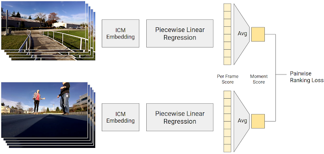
Diagram of the training process for generating frame quality scores. Piecewise linear regression maps from an ICM embedding to a score which, when averaged across a video segment, yields a moment score. The moment score of the preferred segment should be higher.
This process allowed us to train a model that combines the power of Google image recognition technology with the wisdom of human raters–represented by 50 million opinions on what makes interesting content!

While this data-driven score does a great job of identifying interesting (and non-interesting) moments, we also added some bonuses to our overall quality score for phenomena that we know we want Clips to capture, including faces (especially recurring and thus “familiar” ones), smiles, and pets. In our most recent release, we added bonuses for certain activities that customers particularly want to capture, such as hugs, kisses, jumping, and dancing. Recognizing these activities required extensions to the ICM model.

Shot Control
Given this powerful model for predicting the “interestingness” of a scene, the Clips camera can decide which moments to capture in real-time. Its shot control algorithms follow three main principles:
  1. Respect Power & Thermals: We want the Clips battery to last roughly three hours, and we don’t want the device to overheat — the device can’t run at full throttle all the time. Clips spends much of its time in a low-power mode that captures one frame per second. If the quality of that frame exceeds a threshold set by how much Clips has recently shot, it moves into a high-power mode, capturing at 15 fps. Clips then saves a clip at the first quality peak encountered.
  2. Avoid Redundancy: We don’t want Clips to capture all of its moments at once, and ignore the rest of a session. Our algorithms therefore cluster moments into visually similar groups, and limit the number of clips in each cluster.
  3. The Benefit of Hindsight: It’s much easier to determine which clips are the best when you can examine the totality of clips captured. Clips therefore captures more moments than it intends to show to the user. When clips are ready to be transferred to the phone, the Clips device takes a second look at what it has shot, and only transfers the best and least redundant content.
Machine Learning Fairness
In addition to making sure our video dataset represented a diverse population, we also constructed several other tests to assess the fairness of our algorithms. We created controlled datasets by sampling subjects from different genders and skin tones in a balanced manner, while keeping variables like content type, duration, and environmental conditions constant. We then used this dataset to test that our algorithms had similar performance when applied to different groups. To help detect any regressions in fairness that might occur as we improved our moment quality models, we added fairness tests to our automated system. Any change to our software was run across this battery of tests, and was required to pass. It is important to note that this methodology can’t guarantee fairness, as we can’t test for every possible scenario and outcome. However, we believe that these steps are an important part of our long-term work to achieve fairness in ML algorithms.

Conclusion
Most machine learning algorithms are designed to estimate objective qualities – a photo contains a cat, or it doesn’t. In our case, we aim to capture a more elusive and subjective quality – whether a personal photograph is interesting, or not. We therefore combine the objective, semantic content of photographs with subjective human preferences to build the AI behind Google Clips. Also, Clips is designed to work alongside a person, rather than autonomously; to get good results, a person still needs to be conscious of framing, and make sure the camera is pointed at interesting content. We’re happy with how well Google Clips performs, and are excited to continue to improve our algorithms to capture that “perfect” moment!

Acknowledgements
The algorithms described here were conceived and implemented by a large group of Google engineers, research scientists, and others. Figures were made by Lior Shapira. Thanks to Lior and Juston Payne for video content.

Source: Google AI Blog


Custom On-Device ML Models with Learn2Compress


Successful deep learning models often require significant amounts of computational resources, memory and power to train and run, which presents an obstacle if you want them to perform well on mobile and IoT devices. On-device machine learning allows you to run inference directly on the devices, with the benefits of data privacy and access everywhere, regardless of connectivity. On-device ML systems, such as MobileNets and ProjectionNets, address the resource bottlenecks on mobile devices by optimizing for model efficiency. But what if you wanted to train your own customized, on-device models for your personal mobile application?

Yesterday at Google I/O, we announced ML Kit to make machine learning accessible for all mobile developers. One of the core ML Kit capabilities that will be available soon is an automatic model compression service powered by “Learn2Compress” technology developed by our research team. Learn2Compress enables custom on-device deep learning models in TensorFlow Lite that run efficiently on mobile devices, without developers having to worry about optimizing for memory and speed. We are pleased to make Learn2Compress for image classification available soon through ML Kit. Learn2Compress will be initially available to a small number of developers, and will be offered more broadly in the coming months. You can sign up here if you are interested in using this feature for building your own models.

How it Works
Learn2Compress generalizes the learning framework introduced in previous works like ProjectionNet and incorporates several state-of-the-art techniques for compressing neural network models. It takes as input a large pre-trained TensorFlow model provided by the user, performs training and optimization and automatically generates ready-to-use on-device models that are smaller in size, more memory-efficient, more power-efficient and faster at inference with minimal loss in accuracy.
Learn2Compress for automatically generating on-device ML models.
To do this, Learn2Compress uses multiple neural network optimization and compression techniques including:
  • Pruning reduces model size by removing weights or operations that are least useful for predictions (e.g.low-scoring weights). This can be very effective especially for on-device models involving sparse inputs or outputs, which can be reduced up to 2x in size while retaining 97% of the original prediction quality.
  • Quantization techniques are particularly effective when applied during training and can improve inference speed by reducing the number of bits used for model weights and activations. For example, using 8-bit fixed point representation instead of floats can speed up the model inference, reduce power and further reduce size by 4x.
  • Joint training and distillation approaches follow a teacher-student learning strategy — we use a larger teacher network (in this case, user-provided TensorFlow model) to train a compact student network (on-device model) with minimal loss in accuracy.
    Joint training and distillation approach to learn compact student models.
    The teacher network can be fixed (as in distillation) or jointly optimized, and even train multiple student models of different sizes simultaneously. So instead of a single model, Learn2Compress generates multiple on-device models in a single shot, at different sizes and inference speeds, and lets the developer pick one best suited for their application needs.
These and other techniques like transfer learning also make the compression process more efficient and scalable to large-scale datasets.

How well does it work?
To demonstrate the effectiveness of Learn2Compress, we used it to build compact on-device models of several state-of-the-art deep networks used in image and natural language tasks such as MobileNets, NASNet, Inception, ProjectionNet, among others. For a given task and dataset, we can generate multiple on-device models at different inference speeds and model sizes.
Accuracy at various sizes for Learn2Compress models and full-sized baseline networks on CIFAR-10 (left) and ImageNet (right) image classification tasks. Student networks used to produce the compressed variants for CIFAR-10 and ImageNet are modeled using NASNet and MobileNet-inspired architectures, respectively.
For image classification, Learn2Compress can generate small and fast models with good prediction accuracy suited for mobile applications. For example, on ImageNet task, Learn2Compress achieves a model 22x smaller than Inception v3 baseline and 4x smaller than MobileNet v1 baseline with just 4.6-7% drop in accuracy. On CIFAR-10, jointly training multiple Learn2Compress models with shared parameters, takes only 10% more time than training a single Learn2Compress large model, but yields 3 compressed models that are upto 94x smaller in size and upto 27x faster with up to 36x lower cost and good prediction quality (90-95% top-1 accuracy).
Computation cost and average prediction latency (on Pixel phone) for baseline and Learn2Compress models on CIFAR-10 image classification task. Learn2Compress-optimized models use NASNet-style network architecture.
We are also excited to see how well this performs on developer use-cases. For example, Fishbrain, a social platform for fishing enthusiasts, used Learn2Compress to compress their existing image classification cloud model (80MB+ in size and 91.8% top-3 accuracy) to a much smaller on-device model, less than 5MB in size, with similar accuracy. In some cases, we observe that it is possible for the compressed models to even slightly outperform the original large model’s accuracy due to better regularization effects.

We will continue to improve Learn2Compress with future advances in ML and deep learning, and extend to more use-cases beyond image classification. We are excited and looking forward to make this available soon through ML Kit’s compression service on the Cloud. We hope this will make it easy for developers to automatically build and optimize their own on-device ML models so that they can focus on building great apps and cool user experiences involving computer vision, natural language and other machine learning applications.

Acknowledgments
I would like to acknowledge our core contributors Gaurav Menghani, Prabhu Kaliamoorthi and Yicheng Fan along with Wei Chai, Kang Lee, Sheng Xu and Pannag Sanketi. Special thanks to Dave Burke, Brahim Elbouchikhi, Hrishikesh Aradhye, Hugues Vincent, and Arun Venkatesan from the Android team; Sachin Kotwani, Wesley Tarle, Pavel Jbanov and from the Firebase team; Andrei Broder, Andrew Tomkins, Robin Dua, Patrick McGregor, Gaurav Nemade, the Google Expander team and TensorFlow team.


Source: Google AI Blog


Announcing Open Images V4 and the ECCV 2018 Open Images Challenge


In 2016, we introduced Open Images, a collaborative release of ~9 million images annotated with labels spanning thousands of object categories. Since its initial release, we've been hard at work updating and refining the dataset, in order to provide a useful resource for the computer vision community to develop new models

Today, we are happy to announce Open Images V4, containing 15.4M bounding-boxes for 600 categories on 1.9M images, making it the largest existing dataset with object location annotations. The boxes have been largely manually drawn by professional annotators to ensure accuracy and consistency. The images are very diverse and often contain complex scenes with several objects (8 per image on average; visualizer).
Annotated images from the Open Images dataset. Left: Mark Paul Gosselaar plays the guitar by Rhys A. Right: Civilization by Paul Downey. Both images used under CC BY 2.0 license.
In conjunction with this release, we are also introducing the Open Images Challenge, a new object detection challenge to be held at the 2018 European Conference on Computer Vision (ECCV 2018). The Open Images Challenge follows in the tradition of PASCAL VOC, ImageNet and COCO, but at an unprecedented scale.

This challenge is unique in several ways:
  • 12.2M bounding-box annotations for 500 categories on 1.7M training images,
  • A broader range of categories than previous detection challenges, including new objects such as “fedora” and “snowman”.
  • In addition to the object detection main track, the challenge includes a Visual Relationship Detection track, on detecting pairs of objects in particular relations, e.g. “woman playing guitar”.
The training set is available now. A test set of 100k images will be released on July 1st 2018 by Kaggle. Deadline for submission of results is on September 1st 2018. We hope that the very large training set will stimulate research into more sophisticated detection models that will exceed current state-of-the-art performance, and that the 500 categories will enable a more precise assessment of where different detectors perform best. Furthermore, having a large set of images with many objects annotated enables to explore Visual Relationship Detection, which is a hot emerging topic with a growing sub-community.

In addition to the above, Open Images V4 also contains 30.1M human-verified image-level labels for 19,794 categories, which are not part of the Challenge. The dataset includes 5.5M image-level labels generated by tens of thousands of users from all over the world at crowdsource.google.com.

Source: Google AI Blog


Seeing More with In Silico Labeling of Microscopy Images


In the fields of biology and medicine, microscopy allows researchers to observe details of cells and molecules which are unavailable to the naked eye. Transmitted light microscopy, where a biological sample is illuminated on one side and imaged, is relatively simple and well-tolerated by living cultures but produces images which can be difficult to properly assess. Fluorescence microscopy, in which biological objects of interest (such as cell nuclei) are specifically targeted with fluorescent molecules, simplifies analysis but requires complex sample preparation. With the increasing application of machine learning to the field of microscopy, including algorithms used to automatically assess the quality of images and assist pathologists diagnosing cancerous tissue, we wondered if we could develop a deep learning system that could combine the benefits of both microscopy techniques while minimizing the downsides.

With “In Silico Labeling: Predicting Fluorescent Labels in Unlabeled Images”, appearing today in Cell, we show that a deep neural network can predict fluorescence images from transmitted light images, generating labeled, useful, images without modifying cells and potentially enabling longitudinal studies in unmodified cells, minimally invasive cell screening for cell therapies, and investigations using large numbers of simultaneous labels. We also open sourced our network, along with the complete training and test data, a trained model checkpoint, and example code.

Background
Transmitted light microscopy techniques are easy to use, but can produce images in which it can be hard to tell what’s going on. An example is the following image from a phase-contrast microscope, in which the intensity of a pixel indicates the degree to which light was phase-shifted as it passed through the sample.
Transmitted light (phase-contrast) image of a human motor neuron culture derived from induced pluripotent stem cells. Outset 1 shows a cluster of cells, possibly neurons. Outset 2 shows a flaw in the image obscuring underlying cells. Outset 3 shows neurites. Outset 4 shows what appear to be dead cells. Scale bar is 40 μm. Source images for this and the following figures come from the Finkbeiner lab at the Gladstone Institutes.
In the above figure, it’s difficult to tell how many cells are in the cluster in Outset 1, or the locations and states of the cells in Outset 4 (hint: there’s a barely-visible flat cell in the upper-middle). It’s also difficult to get fine structures consistently in focus, such as the neurites in Outset 3.

We can get more information out of transmitted light microscopy by acquiring images in z-stacks: sets of images registered in (x, y) where z (the distance from the camera) is systematically varied. This causes different parts of the cells to come in and out of focus, which provides information about a sample’s 3D structure. Unfortunately, it often takes a trained eye to make sense of the z-stack, and analysis of such z-stacks has largely defied automation. An example z-stack is shown below.
A phase-contrast z-stack of the same cells. Note how the appearance changes as the focus is shifted. Now we can see that the fuzzy shape in the lower right of Outset 1 is a single oblong cell, and that the rightmost cell in Outset 4 is taller than the uppermost cell, possibly indicating that it has undergone programmed cell death.
In contrast, fluorescence microscopy images are easier to analyze, because samples are prepared with carefully engineered fluorescent labels which light up just what the researchers want to see. For example, most human cells have exactly one nucleus, so a nuclear label (such as the blue one below) makes it possible for simple tools to find and count cells in an image.
Fluorescence microscopy image of the same cells. The blue fluorescent label localizes to DNA, highlighting cell nuclei. The green fluorescent label localizes to a protein found only in dendrites, a neural substructure. The red fluorescent label localizes to a protein found only in axons, another neural substructure. With these labels it is much easier to understand what’s happening in the sample. For example, the green and red labels in Outset 1 confirm this is a neural cluster. The red label in Outset 3 shows that the neurites are axons, not dendrites. The upper-left blue dot in Outset 4 reveals a previously hard-to-see nucleus, and the lack of a blue dot for the cell at the left shows it to be DNA-free cellular debris.
However, fluorescence microscopy can have significant downsides. First, there is the complexity and variability introduced by the sample preparation and fluorescent labels themselves. Second, when there are many different fluorescent labels in a sample, spectral overlap can make it hard to tell which color belongs to which label, typically limiting researchers to three or four simultaneous labels in a sample. Third, fluorescence labeling may be toxic to cells and sometimes involves protocols that outright kill them, which makes labeling difficult to use in longitudinal studies where the same cells are followed through time.

Seeing more with deep learning
In our paper, we show that a deep neural network can predict fluorescence images from transmitted light z-stacks. To do this, we created a dataset of transmitted light z-stacks matched to fluorescence images and trained a neural network to predict the fluorescence images from the z-stacks. The following diagram explains the process.
Overview of our system. (A) The dataset of training examples: pairs of transmitted light images from z-stacks with pixel-registered sets of fluorescence images of the same scene. Several different fluorescent labels were used to generate fluorescence images and were varied between training examples; the checkerboard images indicate fluorescent labels which were not acquired for a given example. (B) The untrained deep network was (C) trained on the data A. (D) A z-stack of images of a novel scene. (E) The trained network, C, is used to predict fluorescence labels learned from A for each pixel in the novel images, D.
In the course of this work we developed a new neural network composed of three kinds of basic building-blocks, inspired by the modular design of Inception: an in-scale configuration which does not change the spatial scaling of the features, a down-scale configuration which doubles the spatial scaling, and an up-scale configuration which halves it. This lets us break the hard problem of network architecture design into two easier problems: the arrangement of the building-blocks (macro-architecture), and the design of the building-blocks themselves (micro-architecture). We solved the first problem using design principles discussed in the paper, and the second via an automated search powered by Google Hypertune.

To make sure our method was sound, we validated our model using data from an Alphabet lab as well as two external partners: Steve Finkbeiner's lab at the Gladstone Institutes, and the Rubin Lab at Harvard. These data spanned three transmitted light imaging modalities (bright-field, phase-contrast, and differential interference contrast) and three culture types (human motor neurons derived from induced pluripotent stem cells, rat cortical cultures, and human breast cancer cells). We found that our method can accurately predict several labels including those for nuclei, cell type (e.g. neural), and cell state (e.g. cell death). The following figure shows the model’s predictions alongside the transmitted light input and fluorescence ground-truth for our motor neuron example.
Animation showing the same cells in transmitted light and fluorescence imaging, along with predicted fluorescence labels from our model. Outset 2 shows the model predicts the correct labels despite the artifact in the input image. Outset 3 shows the model infers these processes are axons, possibly because of their distance from the nearest cells. Outset 4 shows the model sees the hard-to-see cell at the top, and correctly identifies the object at the left as DNA-free cell debris.
Try it for yourself!
We’ve open sourced our model, along with our full dataset, code for training and inference, and an example. We’re pleased to report that new labels can be learned with minimal additional training data: in the paper and example code, we show a new label may be learned from a single image. This is due to a phenomenon called transfer learning, where a model can learn a new task more quickly and using less training data if it has already mastered similar tasks.

We hope the ability to generate labeled, useful, images without modifying cells will open up completely new kinds of experiments in biology and medicine. If you’re excited to try this technology in your own work, please read the paper or check out the code!

Acknowledgements
We thank the Google Accelerated Science team for originating and developing this project and its publication, and additionally Kevin P. Murphy for supporting its publication. We thank Mike Ando, Youness Bennani, Amy Chung-Yu Chou, Jason Freidenfelds, Jason Miller, Kevin P. Murphy, Philip Nelson, Patrick Riley, and Samuel Yang for ideas and editing help with this post. This study was supported by NINDS (NS091046, NS083390, NS101995), the NIH’s National Institute on Aging (AG065151, AG058476), the NIH’s National Human Genome Research Institute (HG008105), Google, the ALS Association, and the Michael J. Fox Foundation.