Tag Archives: Computer Vision

Introducing GPipe, an Open Source Library for Efficiently Training Large-scale Neural Network Models


Deep neural networks (DNNs) have advanced many machine learning tasks, including speech recognition, visual recognition, and language processing. Recent advances by BigGan, Bert, and GPT2.0 have shown that ever-larger DNN models lead to better task performance and past progress in visual recognition tasks has also shown a strong correlation between the model size and classification accuracy. For example, the winner of the 2014 ImageNet visual recognition challenge was GoogleNet, which achieved 74.8% top-1 accuracy with 4 million parameters, while just three years later, the winner of the 2017 ImageNet challenge went to Squeeze-and-Excitation Networks, which achieved 82.7% top-1 accuracy with 145.8 million (36x more) parameters. However, in the same period, GPU memory has only increased by a factor of ~3, and the current state-of-the-art image models have already reached the available memory found on Cloud TPUv2s. Hence, there is a strong and pressing need for an efficient, scalable infrastructure that enables large-scale deep learning and overcomes the memory limitation on current accelerators.

Strong correlation between ImageNet accuracy and model size for recently developed representative image classification models
In "GPipe: Efficient Training of Giant Neural Networks using Pipeline Parallelism", we demonstrate the use of pipeline parallelism to scale up DNN training to overcome this limitation. GPipe is a distributed machine learning library that uses synchronous stochastic gradient descent and pipeline parallelism for training, applicable to any DNN that consists of multiple sequential layers. Importantly, GPipe allows researchers to easily deploy more accelerators to train larger models and to scale the performance without tuning hyperparameters. To demonstrate the effectiveness of GPipe, we trained an AmoebaNet-B with 557 million model parameters and input image size of 480 x 480 on Google Cloud TPUv2s. This model performed well on multiple popular datasets, including pushing the single-crop ImageNet accuracy to 84.3%, the CIFAR-10 accuracy to 99%, and the CIFAR-100 accuracy to 91.3%. The core GPipe library has been open sourced under the Lingvo framework.

From Mini- to Micro-Batches
There are two standard ways to speed up moderate-size DNN models. The data parallelism approach employs more machines and splits the input data across them. Another way is to move the model to accelerators, such as GPUs or TPUs, which have special hardware to accelerate model training. However, accelerators have limited memory and limited communication bandwidth with the host machine. Thus, model parallelism is needed for training a bigger DNN model on accelerators by dividing the model into partitions and assigning different partitions to different accelerators. But due to the sequential nature of DNNs, this naive strategy may result in only one accelerator being active during computation, significantly underutilizing accelerator compute capacity. On the other hand, a standard data parallelism approach allows concurrent training of the same model with different input data on multiple accelerators, but cannot increase the maximum model size an accelerator can support.

To enable efficient training across multiple accelerators, GPipe partitions a model across different accelerators and automatically splits a mini-batch of training examples into smaller micro-batches. By pipelining the execution across micro-batches, accelerators can operate in parallel. In addition, gradients are consistently accumulated across micro-batches, so that the number of partitions does not affect the model quality.


Top: The naive model parallelism strategy leads to severe underutilization due to the sequential nature of the network. Only one accelerator is active at a time. Bottom: GPipe divides the input mini-batch into smaller micro-batches, enabling different accelerators to work on separate micro-batches at the same time.
Maximizing Memory and Efficiency
GPipe maximizes memory allocation for model parameters. We ran the experiments on Cloud TPUv2s, each of which has 8 accelerator cores and 64 GB memory (8 GB per accelerator). Without GPipe, a single accelerator can train up to 82 million model parameters due to memory limits. Thanks to recomputation in backpropagation and batch splitting, GPipe reduced intermediate activation memory from 6.26 GB to 3.46GB, enabling 318 million parameters on a single accelerator. We also saw that with pipeline parallelism the maximum model size was proportional to the number of partitions, as expected. With GPipe, AmoebaNet was able to incorporate 1.8 billion parameters on the 8 accelerators of a Cloud TPUv2, 25x times more than is possible without GPipe.

To test efficiency, we measured the effects of GPipe on the model throughput of AmoebaNet-D. Since training required at least two accelerators to fit the model size, we measured the speedup with respect to the naive case with two partitions but no pipeline parallelization. We observed an almost linear speedup in training. Compared to the naive approach with two partitions, distributing the model across four times the accelerators achieved a speedup of 3.5x. While all experiments in our paper used Cloud TPUv2, we see even better performance with the currently available Cloud TPUv3s, each of which has 16 accelerator cores and 256 GB (16 GB per accelerator). GPipe enabled 8 billion parameter Transformer language models on 1024-token sentences with a speedup of 11x when distributing the model across all sixteen accelerators.


Speedup of AmoebaNet-D using GPipe. This model could not fit into one accelerator. The baseline naive-2 is the performance of the native partition approach when the model is split into two partitions. Pipeline-k refers to the performance of GPipe that splits the model into k partitions with k accelerators.
GPipe can also scale training by employing even more accelerators without changes in the hyperparameters. Therefore, it can be combined with data parallelism to scale neural network training using even more accelerators in a complementary way.

Testing Accuracy
We used GPipe to verify the hypothesis that scaling up existing neural networks can achieve even better model quality. We trained an AmoebaNet-B with 557 million model parameters and input image size of 480 x 480 on the ImageNet ILSVRC-2012 dataset. The network was divided into 4 partitions and applied parallel training processes to both model and data. This giant model reached the state-of-the-art 84.3% top-1 / 97% top-5 single-crop validation accuracy without any external data. Large neural networks are not only applicable to datasets like ImageNet, but also relevant for other datasets through transfer learning. It has been shown that better ImageNet models transfer better. We ran transfer learning experiments on the CIFAR10 and CIFAR100 datasets. Our giant models increased the best published CIFAR-10 accuracy to 99% and CIFAR-100 accuracy to 91.3%.

Conclusion
The ongoing development and success of many practical machine learning applications, such as autonomous driving and medical imaging, depend on achieving the highest accuracy possible. As this often requires building larger and even more complex models, we are happy to provide GPipe to the broader research community, and hope it is a useful infrastructure for efficient training of large-scale DNNs.

Acknowledgments
Special thanks to the co-authors of the paper: Youlong Cheng, Dehao Che, HyoukJoong Lee, Jiquan Ngiam, Quoc V. Le, and Zhifeng Chen. We wish to thank Esteban Real, Alok Aggarwal, Xiaodan Song, Naveen Kumar, Mark Heffernan, Rajat Monga, Megan Kacholia, Samy Bengio, and Jeff Dean for their support and valuable input; Noam Shazeer, Patrick Nguyen, Xiaoqiang Zheng, Yonghui Wu, Barret Zoph, Ekin Cubuk, Jonathan Shen, Tianqi Chen, and Vijay Vasudevan for helpful discussions and inspirations; and the larger Google Brain team.

Source: Google AI Blog


Using Global Localization to Improve Navigation


One of the consistent challenges when navigating with Google Maps is figuring out the right direction to go: sure, the app tells you to go north - but many times you're left wondering, "Where exactly am I, and which way is north?" Over the years, we've attempted to improve the accuracy of the blue dot with tools like GPS and compass, but found that both have physical limitations that make solving this challenge difficult, especially in urban environments.

We're experimenting with a way to solve this problem using a technique we call global localization, which combines Visual Positioning Service (VPS), Street View, and machine learning to more accurately identify position and orientation. Using the smartphone camera as a sensor, this technology enables a more powerful and intuitive way to help people quickly determine which way to go.
Due to limitations with accuracy and orientation, guidance via GPS alone is limited in urban environments. Using VPS, Street View and machine learning, Global Localization can provide better context on where you are relative to where you're going.
In this post, we'll discuss some of the limitations of navigation in urban environments and how global localization can help overcome them.

Where GPS Falls Short
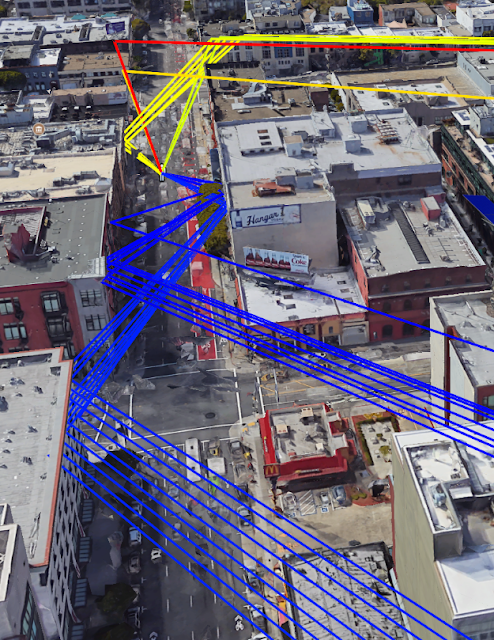
The process of identifying the position and orientation of a device relative to some reference point is referred to as localization. Various techniques approach localization in different ways. GPS relies on measuring the delay of radio signals from multiple dedicated satellites to determine a precise location. However, in dense urban environments like New York or San Francisco, it can be incredibly hard to pinpoint a geographic location due to low visibility to the sky and signals reflecting off of buildings. This can result in highly inaccurate placements on the map, meaning that your location could appear on the wrong side of the street, or even a few blocks away.
GPS signals bouncing off facades in an urban environment.
GPS has another technical shortcoming: it can only determine the location of the device, not the orientation. Sometimes, sensors in your mobile device can remedy the situation by measuring the magnetic and gravity field of the earth and the relative motion of the device in order to give rough estimates of your orientation. But these sensors are easily skewed by magnetic objects such as cars, pipes, buildings, and even electrical wires inside the phone, resulting in errors that can be inaccurate by up to 180 degrees.

A New Approach to Localization
To improve the precision position and orientation of the blue dot on the map, a new complementary technology is necessary. When walking down the street, you orient yourself by comparing what you see with what you expect to see. Global localization uses a combination of techniques that enable the camera on your mobile device to orient itself much as you would.

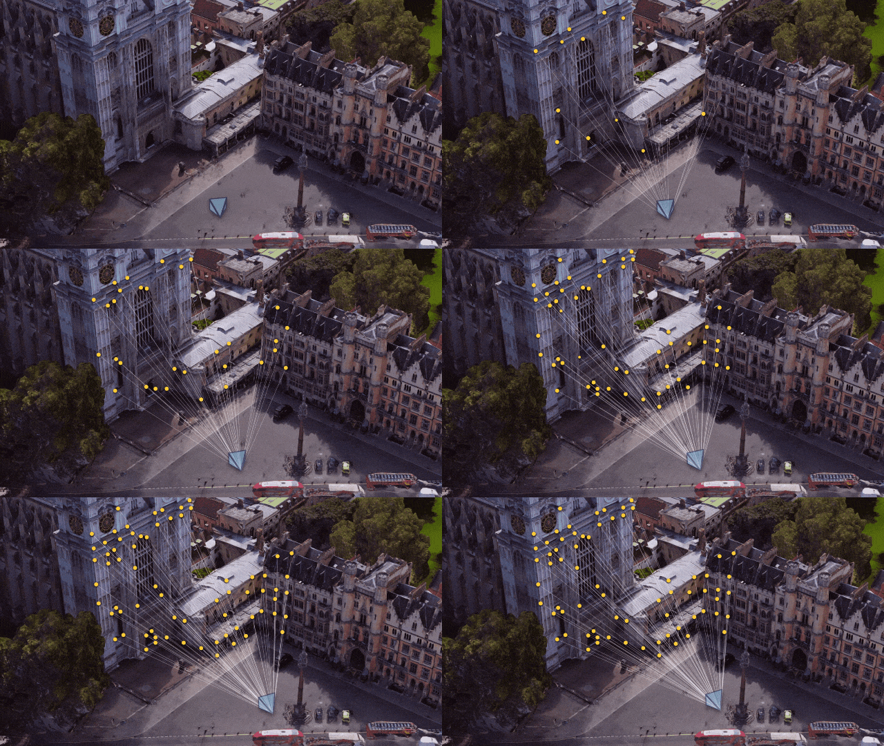
VPS determines the location of a device based on imagery rather than GPS signals. VPS first creates a map by taking a series of images which have a known location and analyzing them for key visual features, such as the outline of buildings or bridges, to create a large scale and fast searchable index of those visual features. To localize the device, VPS compares the features in imagery from the phone to those in the VPS index. However, the accuracy of localization through VPS is greatly affected by the quality of the both the imagery and the location associated with it. And that poses another question—where does one find an extensive source of high-quality global imagery?

Enter Street View
Over 10 years ago we launched Street View in Google Maps in order to help people explore the world more deeply. In that time, Street View has continued to expand its coverage of the world, empowering people to not only preview their route, but also step inside famous landmarks and museums, no matter where they are. To deliver global localization with VPS, we connected it with Street View data, making use of information gathered and tested from over 93 countries across the globe. This rich dataset provides trillions of strong reference points to apply triangulation, helping more accurately determine the position of a device and guide people towards their destination.
Features matched from multiple images.
Although this approach works well in theory, making it work well in practice is a challenge. The problem is that the imagery from the phone at the time of localization may differ from what the scene looked like when the Street View imagery was collected, perhaps months earlier. For example, trees have lots of rich detail, but change as the seasons change and even as the wind blows. To get a good match, we need to filter out temporary parts of the scene and focus on permanent structure that doesn't change over time. That's why a core ingredient in this new approach is applying machine learning to automatically decide which features to pay attention to, prioritizing features that are likely to be permanent parts of the scene and ignoring things like trees, dynamic light movement, and construction that are likely transient. This is just one of the many ways in which we use machine learning to improve accuracy.

Combining Global Localization with Augmented Reality
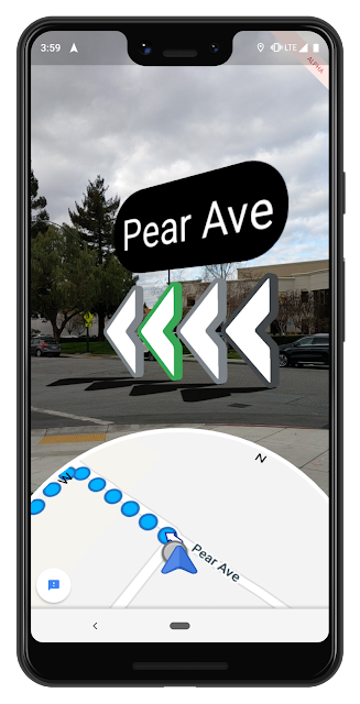
Global localization is an additional option that users can enable when they most need accuracy. And, this increased precision has enabled the possibility of a number of new experiences. One of the newest features we're testing is the ability to use ARCore, Google's platform for building augmented reality experiences, to overlay directions right on top of Google Maps when someone is in walking navigation mode. With this feature, a quick glance at your phone shows you exactly which direction you need to go.
Although early results are promising, there's significant work to be done. One outstanding challenge is making this technology work everywhere, in all types of conditions—think late at night, in a snowstorm, or in torrential downpour. To make sure we're building something that's truly useful, we're starting to test this feature with select Local Guides, a small group of Google Maps enthusiasts around the world who we know will offer us the feedback about how this approach can be most helpful.

Like other AI-driven camera experiences such as Google Lens (which uses the camera to let you search what you see), we believe the ability to overlay directions over the real world environment offers an exciting and useful way to use the technology that already exists in your pocket. We look forward to continuing to develop this technology, and the potential for smartphone cameras to add new types of valuable experiences.

Source: Google AI Blog


Top Shot on Pixel 3


Life is full of meaningful moments — from a child’s first step to an impromptu jump for joy — that one wishes could be preserved with a picture. However, because these moments are often unpredictable, missing that perfect shot is a frustrating problem that smartphone camera users face daily. Using our experience from developing Google Clips, we wondered if we could develop new techniques for the Pixel 3 camera that would allow everyone to capture the perfect shot every time.

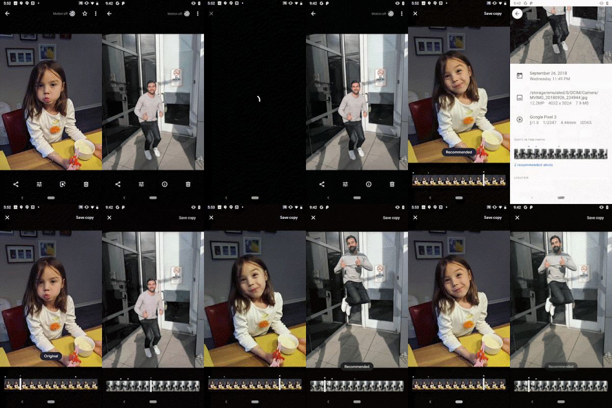
Top Shot is a new feature recently launched with Pixel 3 that helps you to capture precious moments precisely and automatically at the press of the shutter button. Top Shot saves and analyzes the image frames before and after the shutter press on the device in real-time using computer vision techniques, and recommends several alternative high-quality HDR+ photos.
Examples of Top Shot on Pixel 3. On the left, a better smiling shot is recommended. On the right, a better jump shot is recommended. The recommended images are high-quality HDR+ shots.
Capturing Multiple Moments
When a user opens the Pixel 3 Camera app, Top Shot is enabled by default, helping to capture the perfect moment by analyzing images taken both before and after the shutter press. Each image is analyzed for some qualitative features (e.g., whether the subject is smiling or not) in real-time and entirely on-device to preserve privacy and minimize latency. Each image is also associated with additional signals, such as optical flow of the image, exposure time, and gyro sensor data to form the input features used to score the frame quality.

When you press the shutter button, Top Shot captures up to 90 images from 1.5 seconds before and after the shutter press, selecting up to two alternative shots to save in high resolution — the original shutter frame and high-res alternatives for you to review (other lower-res frames can also be reviewed as desired). The shutter frame is processed and saved first. The best alternative shots are saved afterwards. Google’s Visual Core on Pixel 3 is used to process these top alternative shots as HDR+ images with a very small amount of extra latency, and are embedded into the file of the Motion Photo.
Top-level diagram of Top Shot capture.
Given Top Shot runs in the camera as a background process, it must have very low power consumption. As such, Top Shot uses a hardware-accelerated MobileNet-based single shot detector (SSD). The execution of such optimized models is also throttled by power and thermal limits.

Recognizing Top Moments
When we set out to understand how to enable people to capture the best moments with their camera, we focused on three key attributes: 1) functional qualities like lighting, 2) objective attributes (are the subject's eyes open? Are they smiling?), and 3) subjective qualities like emotional expressions. We designed a computer vision model to recognize these attributes while operating in a low-latency, on-device mode.

During our development process, we started with a vanilla MobileNet model and set out to optimize for Top Shot, arriving at a customized architecture that operated within our accuracy, latency and power tradeoff constraints. Our neural network design detects low-level visual attributes in early layers, like whether the subject is blurry, and then dedicates additional compute and parameters toward more complex objective attributes like whether the subject's eyes are open, and subjective attributes like whether there is an emotional expression of amusement or surprise. We trained our model using knowledge distillation over a large number of diverse face images using quantization during both training and inference.

We then adopted a layered Generalized Additive Model (GAM) to provide quality scores for faces and combine them into a weighted-average “frame faces” score. This model made it easy for us to interpret and identify the exact causes of success or failure, enabling rapid iteration to improve the quality and performance of our attributes model. The number of free parameters was on the order of dozens, so we could optimize these using Google's black box optimizer, Vizier, in tandem with any other parameters that affected selection quality.

Frame Scoring Model
While Top Shot prioritizes for face analysis, there are good moments in which faces are not the primary subject. To handle those use cases, we include the following additional scores in the overall frame quality score:
  • Subject motion saliency score — the low-resolution optical flow between the current frame and the previous frame is estimated in ISP to determine if there is salient object motion in the scene.
  • Global motion blur score — estimated from the camera motion and the exposure time. The camera motion is calculated from sensor data from the gyroscope and OIS (optical image stabilization).
  • “3A” scores — the status of auto exposure, auto focus, and auto white balance, are also considered.
All the individual scores are used to train a model predicting an overall quality score, which matches the frame preference of human raters, to maximize end-to-end product quality.

End-to-End Quality and Fairness
Most of the above components are each evaluated for accuracy independently However, Top Shot presents requirements that are uniquely challenging since it’s running real-time in the Pixel Camera. Additionally, we needed to ensure that all these signals are combined in a system with favorable results. That means we need to gauge our predictions against what our users perceive as the “top shot.”

To test this, we collected data from hundreds of volunteers, along with their opinions of which frames (out of up to 90!) looked best. This donated dataset covers many typical use cases, e.g. portraits, selfies, actions, landscapes, etc.

Many of the 3-second clips provided by Top Shot had more than one good shot, so it was important for us to engineer our quality metrics to handle this. We used some modified versions of traditional Precision and Recall, some classic ranking metrics (such as Mean Reciprocal Rank), and a few others that were designed specifically for the Top Shot task as our objective. In addition to these metrics, we additionally investigated causes of image quality issues we saw during development, leading to improvements in avoiding blur, handling multiple faces better, and more. In doing so, we were able to steer the model towards a set of selections people were likely to rate highly.

Importantly, we tested the Top Shot system for fairness to make sure that our product can offer a consistent experience to a very wide range of users. We evaluated the accuracy of each signal used in Top Shot on several different subgroups of people (based on gender, age, ethnicity, etc), testing for accuracy of each signal across those subgroups.

Conclusion
Top Shot is just one example of how Google leverages optimized hardware and cutting-edge machine learning to provide useful tools and services. We hope you’ll find this feature useful, and we’re committed to further improving the capabilities of mobile phone photography!

Acknowledgements
This post reflects the work of a large group of Google engineers, research scientists, and others including: Ari Gilder, Aseem Agarwala, Brendan Jou, David Karam, Eric Penner, Farooq Ahmad, Henri Astre, Hillary Strickland, Marius Renn, Matt Bridges, Maxwell Collins, Navid Shiee, Ryan Gordon, Sarah Clinckemaillie, Shu Zhang, Vivek Kesarwani, Xuhui Jia, Yukun Zhu, Yuzo Watanabe and Chris Breithaupt.

Source: Google AI Blog


Learning to Predict Depth on the Pixel 3 Phones


Portrait Mode on the Pixel smartphones lets you take professional-looking images that draw attention to a subject by blurring the background behind it. Last year, we described, among other things, how we compute depth with a single camera using its Phase-Detection Autofocus (PDAF) pixels (also known as dual-pixel autofocus) using a traditional non-learned stereo algorithm. This year, on the Pixel 3, we turn to machine learning to improve depth estimation to produce even better Portrait Mode results.
Left: The original HDR+ image. Right: A comparison of Portrait Mode results using depth from traditional stereo and depth from machine learning. The learned depth result has fewer errors. Notably, in the traditional stereo result, many of the horizontal lines behind the man are incorrectly estimated to be at the same depth as the man and are kept sharp.
(Mike Milne)
A Short Recap
As described in last year’s blog post, Portrait Mode uses a neural network to determine what pixels correspond to people versus the background, and augments this two layer person segmentation mask with depth information derived from the PDAF pixels. This is meant to enable a depth-dependent blur, which is closer to what a professional camera does.

PDAF pixels work by capturing two slightly different views of a scene, shown below. Flipping between the two views, we see that the person is stationary, while the background moves horizontally, an effect referred to as parallax. Because parallax is a function of the point’s distance from the camera and the distance between the two viewpoints, we can estimate depth by matching each point in one view with its corresponding point in the other view.
The two PDAF images on the left and center look very similar, but in the crop on the right you can see the parallax between them. It is most noticeable on the circular structure in the middle of the crop.
However, finding these correspondences in PDAF images (a method called depth from stereo) is extremely challenging because scene points barely move between the views. Furthermore, all stereo techniques suffer from the aperture problem. That is, if you look at the scene through a small aperture, it is impossible to find correspondence for lines parallel to the stereo baseline, i.e., the line connecting the two cameras. In other words, when looking at the horizontal lines in the figure above (or vertical lines in portrait orientation shots), any proposed shift of these lines in one view with respect to the other view looks about the same. In last year’s Portrait Mode, all these factors could result in errors in depth estimation and cause unpleasant artifacts.

Improving Depth Estimation
With Portrait Mode on the Pixel 3, we fix these errors by utilizing the fact that the parallax used by depth from stereo algorithms is only one of many depth cues present in images. For example, points that are far away from the in-focus plane appear less sharp than ones that are closer, giving us a defocus depth cue. In addition, even when viewing an image on a flat screen, we can accurately tell how far things are because we know the rough size of everyday objects (e.g. one can use the number of pixels in a photograph of a person’s face to estimate how far away it is). This is called a semantic cue.

Designing a hand-crafted algorithm to combine these different cues is extremely difficult, but by using machine learning, we can do so while also better exploiting the PDAF parallax cue. Specifically, we train a convolutional neural network, written in TensorFlow, that takes as input the PDAF pixels and learns to predict depth. This new and improved ML-based method of depth estimation is what powers Portrait Mode on the Pixel 3.
Our convolutional neural network takes as input the PDAF images and outputs a depth map. The network uses an encoder-decoder style architecture with skip connections and residual blocks.
Training the Neural Network
In order to train the network, we need lots of PDAF images and corresponding high-quality depth maps. And since we want our predicted depth to be useful for Portrait Mode, we also need the training data to be similar to pictures that users take with their smartphones.

To accomplish this, we built our own custom “Frankenphone” rig that contains five Pixel 3 phones, along with a Wi-Fi-based solution that allowed us to simultaneously capture pictures from all of the phones (within a tolerance of ~2 milliseconds). With this rig, we computed high-quality depth from photos by using structure from motion and multi-view stereo.
Left: Custom rig used to collect training data. Middle: An example capture flipping between the five images. Synchronization between the cameras ensures that we can calculate depth for dynamic scenes, such as this one. Right: Ground truth depth. Low confidence points, i.e., points where stereo matches are not reliable due to weak texture, are colored in black and are not used during training. (Sam Ansari and Mike Milne)
The data captured by this rig is ideal for training a network for the following main reasons:
  • Five viewpoints ensure that there is parallax in multiple directions and hence no aperture problem.
  • The arrangement of the cameras ensures that a point in an image is usually visible in at least one other image resulting in fewer points with no correspondences.
  • The baseline, i.e., the distance between the cameras is much larger than our PDAF baseline resulting in more accurate depth estimation.
  • Synchronization between the cameras ensure that we can calculate depth for dynamic scenes like the one above.
  • Portability of the rig ensures that we can capture photos in the wild simulating the photos users take with their smartphones.
However, even though the data captured from this rig is ideal, it is still extremely challenging to predict the absolute depth of objects in a scene — a given PDAF pair can correspond to a range of different depth maps (depending on lens characteristics, focus distance, etc). To account for this, we instead predict the relative depths of objects in the scene, which is sufficient for producing pleasing Portrait Mode results.

Putting it All Together
This ML-based depth estimation needs to run fast on the Pixel 3, so that users don’t have to wait too long for their Portrait Mode shots. However, to get good depth estimates that makes use of subtle defocus and parallax cues, we have to feed full resolution, multi-megapixel PDAF images into the network. To ensure fast results, we use TensorFlow Lite, a cross-platform solution for running machine learning models on mobile and embedded devices and the Pixel 3’s powerful GPU to compute depth quickly despite our abnormally large inputs. We then combine the resulting depth estimates with masks from our person segmentation neural network to produce beautiful Portrait Mode results.

Try it Yourself
In Google Camera App version 6.1 and later, our depth maps are embedded in Portrait Mode images. This means you can use the Google Photos depth editor to change the amount of blur and the focus point after capture. You can also use third-party depth extractors to extract the depth map from a jpeg and take a look at it yourself. Also, here is an album showing the relative depth maps and the corresponding Portrait Mode images for traditional stereo and the learning-based approaches.

Acknowledgments
This work wouldn’t have been possible without Sam Ansari, Yael Pritch Knaan, David Jacobs, Jiawen Chen, Juhyun Lee and Andrei Kulik. Special thanks to Mike Milne and Andy Radin who captured data with the five-camera rig.

Source: Google AI Blog


A Structured Approach to Unsupervised Depth Learning from Monocular Videos


Perceiving the depth of a scene is an important task for an autonomous robot — the ability to accurately estimate how far from the robot objects are, is crucial for obstacle avoidance, safe planning and navigation. While depth can be obtained (and learned) from sensor data, such as LIDAR, it is also possible to learn it in an unsupervised manner from a monocular camera only, relying on the motion of the robot and the resulting different views of the scene. In doing so, the “ego-motion” (the motion of the robot/camera between two frames) is also learned, which provides localization of the robot itself. While this approach has a long history — coming from the structure-from-motion and multi-view geometry paradigms — new learning based techniques, more specifically for unsupervised learning of depth and ego-motion by using deep neural networks, have advanced the state of the art, including work by Zhou et al., and our own prior research which aligns 3D point clouds of the scene during training.

Despite these efforts, learning to predict scene depth and ego-motion remains an ongoing challenge, specifically when handling highly dynamic scenes and estimating proper depth of moving objects. Because previous research efforts for unsupervised monocular learning do not model moving objects, it can result in consistent misestimation of objects’ depth, often resulting in mapping their depth to infinity.

In “Depth Prediction Without the Sensors: Leveraging Structure for Unsupervised Learning from Monocular Videos”, to appear in AAAI 2019, we propose a novel approach which is able to model moving objects and produces high quality depth estimation results. Our approach is able to recover the correct depth for moving objects compared to previous methods for unsupervised learning from monocular videos. In our paper, we also propose a seamless online refinement technique that can further improve quality and be applied for transfer across datasets. Furthermore, to encourage even more advanced approaches of onboard robotics learning, we have open sourced the code in TensorFlow.
Previous work (middle row) has not been able to correctly estimate depth of moving objects mapping them to infinity (dark blue regions in the heatmap). Our approach (right) provides much better depth estimates.
Structure
A key idea in our approach is to introduce structure into the learning framework. That is, instead of relying on a neural network to learn depth directly, we treat the monocular scene as 3D, composed of moving objects, including the robot itself. The respective motions are modeled as independent transformations — rotations and translations — in the scene, which is then used to model the 3D geometry and estimate all the objects’ motions. Additionally, knowing which objects may potentially move (e.g., cars, people, bicycles, etc.) helps us learn separate motion vectors for them even if they may be static. By decomposing the scene into 3D and individual objects, better depth and ego-motion in the scene is learned, especially on very dynamic scenes.

We tested this method on both KITTI and Cityscapes urban driving datasets, and found that it outperforms state-of-the-art approaches, and is approaching in quality methods which used stereo pair videos as training supervision. Importantly, we are able to recover correctly the depth of a car moving at the same speed as the ego-motion vehicle. This has been challenging previously — in this case, the moving vehicle appears (in a monocular input) as static, exhibiting the same behavior as the static horizon, resulting in an inferred infinite depth. While stereo inputs can solve that ambiguity, our approach is the first one that is able to correctly infer that from a monocular input.
Previous work with monocular inputs were not able to extract moving objects and incorrectly map them to infinity.
Furthermore, since objects are treated individually in our method, the algorithm is able to provide for the motion vectors for each individual object, i.e. which is an estimate of where it is heading:
Example depth results for a dynamic scene together with estimates of the motion vectors of the individual objects (rotation angles are estimated too, but for simplicity are not shown).
In addition to these results, this research provides motivation for further exploring what an unsupervised learning approach can achieve, as monocular inputs are cheaper and easier to deploy than stereo or LIDAR sensors. As can be seen in the figures below, in both the KITTI and Cityscapes datasets, the supervision sensor (be it stereo or LIDAR) is missing values and may occasionally be misaligned with the camera input, which happens due to time delay.
Depth prediction from monocular video input on the KITTI dataset, middle row, compared to ground truth depth from a Lidar sensor; the latter does not cover the full scene and has missing and noisy values. Ground truth depth is not used during training.
Depth prediction on the Cityscapes dataset. Left to right: image, baseline, our method and ground truth provided by stereo. Note the missing values in the stereo ground truth. Also note that our algorithm is able to achieve these results without any ground truth depth supervision.
Ego-motion
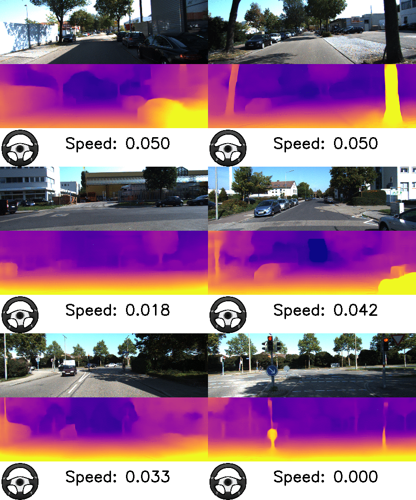
Our results also provide the best among the state-of-the-art estimates in ego-motion, which is crucial for autonomous robots, as it provides localization of the robots while moving in the environment. The video below shows results from our method that visualizes the speed and turning angle, obtained from the inferred ego-motion. While the outputs of both depth and ego-motion are valid up to a scalar, we can see that it is able to estimate its relative speed when slowing down and stopping.
Depth and ego-motion prediction. Follow the speed and the turning angle indicator to see the estimates when the car is taking a turn or stopping for a red light.
Transfer Across Domains
An important characteristic of a learning algorithm is its adaptability when moved to an unknown environment. In this work we further introduce an online refinement approach which continues to learn online while collecting new data. Below are examples of improvement of the estimated depth quality, after training on Cityscapes and online refinement on KITTI.
Online refinement when training on the Cityscapes Data and testing on KITTI. The images show depth prediction of the trained model, and of the trained model with online refinement. Depth prediction with online refinement better outlines the objects in the scene.
We further tested on a notably different dataset and setting, i.e. on an indoor dataset collected by the Fetch robot, while the training is done on the outdoor urban driving Cityscapes dataset. As to be expected, there is a large discrepancy between these datasets. Despite this, we observe that the online learning technique is able to obtain better depth estimates than the baseline.
Results of online adaptation when transferring the learning model from Cityscapes (an outdoors dataset collected from a moving car) to a dataset collected indoors by the Fetch robot. The bottom row shows improved depth after applying online refinement.
In summary, this work addresses unsupervised learning of depth and ego-motion from a monocular camera, and tackles the problem in highly dynamic scenes. It achieves high quality depth and ego-motion results and with quality comparable to stereo and sets forward the idea of incorporating structure in the learning process. More notably, our proposed combination of unsupervised learning of depth and ego-motion from monocular video only and online adaptation demonstrates a powerful concept, because not only can it learn in unsupervised manner from simple video, but it can also be transferred easily to other datasets.

Acknowledgements
This research was conducted by Vincent Casser, Soeren Pirk, Reza Mahjourian and Anelia Angelova. We would like to thank Ayzaan Wahid for his help with data collection and Martin Wicke and Vincent Vanhoucke for their support and encouragement.

Source: Google AI Blog


Fluid Annotation: An Exploratory Machine Learning–Powered Interface for Faster Image Annotation


The performance of modern deep learning–based computer vision models, such as those implemented by the TensorFlow Object Detection API, depends on the availability of increasingly large, labeled training datasets, such as Open Images. However, obtaining high-quality training data is quickly becoming a major bottleneck in computer vision. This is especially the case for pixel-wise prediction tasks such as semantic segmentation, used in applications such as autonomous driving, robotics, and image search. Indeed, traditional manual labeling tools require an annotator to carefully click on the boundaries to outline each object in the image, which is tedious: labeling a single image in the COCO+Stuff dataset takes 19 minutes, while labeling the whole dataset would take over 53k hours!
Example of image in the COCO dataset (left) and its pixel-wise semantic labeling (right). Image credit: Florida Memory, original image.
In “Fluid Annotation: A Human-Machine Collaboration Interface for Full Image Annotation”, to be presented at the Brave New Ideas track of the 2018 ACM Multimedia Conference, we explore a machine learning–powered interface for annotating the class label and outline of every object and background region in an image, accelerating the creation of labeled datasets by a factor of 3x.

Fluid Annotation starts from the output of a strong semantic segmentation model, which a human annotator can modify through machine-assisted edit operations using a natural user interface. Our interface empowers annotators to choose what to correct and in which order, allowing them to effectively focus their efforts on what the machine does not already know.
Visualization of the fluid annotation interface in action on image from COCO dataset. Image credit: gamene, original image.
More precisely, to annotate an image we first run it through a pre-trained semantic segmentation model (Mask-RCNN). This generates around 1000 image segments with their class labels and confidence scores. The segments with the highest confidences are used to initialize the labeling which is presented to the annotator. Afterwards, the annotator can: (1) Change the label of an existing segment choosing from a shortlist generated by the machine. (2) Add a segment to cover a missing object. The machine identifies the most likely pre-generated segments, through which the annotator can scroll and select the best one. (3) Remove an existing segment. (4) Change the depth-order of overlapping segments. To get a better feeling for this interface, try out the demo (desktop only).
Comparison of annotations using traditional manual labeling tools (middle column) and fluid annotation (right) on three COCO images. While object boundaries are often more accurate when using manual labeling tools, the biggest source of annotation differences is because human annotators often disagree on the exact object class. Image Credits: sneaka, original image (top), Dan Hurt, original image (middle), Melodie Mesiano, original image (bottom).
Fluid Annotation is a first exploratory step towards making image annotation faster and easier. In future work we aim to improve the annotation of object boundaries, make the interface faster by including more machine intelligence, and finally extend the interface to handle previous unseen classes for which efficient data collection is needed the most.

Acknowledgements
This work was done in collaboration with Misha Andriluka. Special thanks to Christine Sugrue for creating the fluid annotation demo. We also thank Anna Ukhanova and Damien Henry for their valuable input.

Source: Google AI Blog


Conceptual Captions: A New Dataset and Challenge for Image Captioning


The web is filled with billions of images, helping to entertain and inform the world on a countless variety of subjects. However, much of that visual information is not accessible to those with visual impairments, or with slow internet speeds that prohibit the loading of images. Image captions, manually added by website authors using Alt-text HTML, is one way to make this content more accessible, so that a natural-language description for images that can be presented using text-to-speech systems. However, existing human-curated Alt-text HTML fields are added for only a very small fraction of web images. And while automatic image captioning can help solve this problem, accurate image captioning is a challenging task that requires advancing the state of the art of both computer vision and natural language processing.
Image captioning can help millions with visual impairments by converting images captions to text. Image by Francis Vallance (Heritage Warrior), used under CC BY 2.0 license.
Today we introduce Conceptual Captions, a new dataset consisting of ~3.3 million image/caption pairs that are created by automatically extracting and filtering image caption annotations from billions of web pages. Introduced in a paper presented at ACL 2018, Conceptual Captions represents an order of magnitude increase of captioned images over the human-curated MS-COCO dataset. As measured by human raters, the machine-curated Conceptual Captions has an accuracy of ~90%. Furthermore, because images in Conceptual Captions are pulled from across the web, it represents a wider variety of image-caption styles than previous datasets, allowing for better training of image captioning models. To track progress on image captioning, we are also announcing the Conceptual Captions Challenge for the machine learning community to train and evaluate their own image captioning models on the Conceptual Captions test bed.
Illustration of images and captions in the Conceptual Captions dataset.
Clockwise from top left, images by Jonny Hunter, SigNote Cloud, Tony Hisgett, ResoluteSupportMedia. All images used under CC BY 2.0 license
Generating the Dataset
To generate the Conceptual Captions dataset, we start by sourcing images from the web that have Alt-text HTML attributes. We automatically screen these for certain properties to ensure image quality while also avoiding undesirable content such as adult themes. We then apply text-based filtering, removing captions with non-descriptive text (such as hashtags, poor grammar or added language that does not relate to the image); we also discard texts with high sentiment polarity or adult content (for more details on the filtering criteria, please see our paper). We use existing image classification models to make sure that, for any given image, there is overlap between its Alt-text (allowing for word variations) and the labels that the image classifier outputs for that image.

From Specific Names to General Concepts
While candidates passing the above filters tend to be good Alt-text image descriptions, a large majority use proper names (for people, venues, locations, organizations etc.). This is problematic because it is very difficult for an image captioning model to learn such fine-grained proper name inference from input image pixels, and also generate natural-language descriptions simultaneously1.

To address the above problems we wrote software that automatically replaces proper names with words representing the same general notion, i.e., with their concept. In some cases, the proper names are removed to simplify the text. For example, we substitute people names (e.g., “Former Miss World Priyanka Chopra on the red carpet” becomes “actor on the red carpet”), remove locations names (“Crowd at a concert in Los Angeles” becomes “Crowd at a concert”), remove named modifiers (e.g., “Italian cuisine” becomes just “cuisine”) and correct newly formed noun phrases if needed (e.g., “artist and artist” becomes “artists”, see the example illustration below).
Illustration of text modification. Image by Rockoleando used under CC BY 2.0 license.
Finally, we cluster all resolved entities (e.g., “artist”, “dog”, “neighborhood”, etc.) and keep only the candidate types which have a count of over 100 mentions, a quantity sufficient to support representation learning for these entities. This retained around 16K entity concepts such as: “person”, “actor”, “artist”, “player” and “illustration”. Less frequent ones that we retained include “baguette”, “bridle”, “deadline”, “ministry” and “funnel”.

In the end, it required roughly one billion (English) webpages containing over 5 billion candidate images to obtain a clean and learnable image caption dataset of over 3M samples (a rejection rate of 99.94%). Our control parameters were biased towards high precision, although these can be tuned to generate an order of magnitude more examples with lower precision.

Dataset Impact
To test the usefulness of our dataset, we independently trained both RNN-based, and Transformer-based image captioning models implemented in Tensor2Tensor (T2T), using the MS-COCO dataset (using 120K images with 5 human annotated-captions per image) and the new Conceptual Captions dataset (using over 3.3M images with 1 caption per image). See our paper for more details on model architectures.

These models were tested using images from Flickr30K dataset (which are out-of-domain for both MS-COCO and Conceptual Captions), and the resulting captions evaluated using 3 human raters per test case. The results are reported in the table below.
From these results we conclude that models trained on Conceptual Captions generalized better than competing approaches irrespective of the architecture (i.e., RNN or Transformer). In addition, we found that Transformer models did better than RNN when trained on either dataset. The conclusion from these findings is that Conceptual Captions provides the ability to train image captioning models that perform better on a wide variety of images.

Get Involved
It is our hope that this dataset will help the machine learning community advance the state of the art in image captioning models. Importantly, since no human annotators were involved in its creation, this dataset is highly scalable, potentially allowing the expansion of the dataset to enable automatic creation of Alt-text-HTML-like descriptions for an even wider variety of images. We encourage all those interested to partake in the Conceptual Captions Challenge, and we look forward to seeing what the community can do! For more details and the latest results please visit the challenge website.

Acknowledgements
Thanks to Nan Ding, Sebastian Goodman and Bo Pang for training models with Conceptual Captions dataset, and to Amol Wankhede for driving the public release efforts for the dataset.


1 In our paper, we posit that if automatic determination of names, locations, brands, etc. from the image is needed, it should be done as a separate task that may leverage image meta-information (e.g. GPS info), or complementary techniques such as OCR.

Source: Google AI Blog


MnasNet: Towards Automating the Design of Mobile Machine Learning Models


Convolutional neural networks (CNNs) have been widely used in image classification, face recognition, object detection and many other domains. Unfortunately, designing CNNs for mobile devices is challenging because mobile models need to be small and fast, yet still accurate. Although significant effort has been made to design and improve mobile models, such as MobileNet and MobileNetV2, manually creating efficient models remains challenging when there are so many possibilities to consider. Inspired by recent progress in AutoML neural architecture search, we wondered if the design of mobile CNN models could also benefit from an AutoML approach.

In “MnasNet: Platform-Aware Neural Architecture Search for Mobile”, we explore an automated neural architecture search approach for designing mobile models using reinforcement learning. To deal with mobile speed constraints, we explicitly incorporate the speed information into the main reward function of the search algorithm, so that the search can identify a model that achieves a good trade-off between accuracy and speed. In doing so, MnasNet is able to find models that run 1.5x faster than state-of-the-art hand-crafted MobileNetV2 and 2.4x faster than NASNet, while reaching the same ImageNet top 1 accuracy.

Unlike in previous architecture search approaches, where model speed is considered via another proxy (e.g., FLOPS), our approach directly measures model speed by executing the model on a particular platform, e.g., Pixel phones which were used in this research study. In this way, we can directly measure what is achievable in real-world practice, given that each type of mobile devices has its own software and hardware idiosyncrasies and may require different architectures for the best trade-offs between accuracy and speed.

The overall flow of our approach consists mainly of three components: a RNN-based controller for learning and sampling model architectures, a trainer that builds and trains models to obtain the accuracy, and an inference engine for measuring the model speed on real mobile phones using TensorFlow Lite. We formulate a multi-objective optimization problem that aims to achieve both high accuracy and high speed, and utilize a reinforcement learning algorithm with a customized reward function to find Pareto optimal solutions (e.g., models that have the highest accuracy without worsening speed).
Overall flow of our automated neural architecture search approach for Mobile.
In order to strike the right balance between search flexibility and search space size, we propose a novel factorized hierarchical search space, which factorizes a convolutional neural network into a sequence of blocks, and then uses a hierarchical search space to determine the layer architecture for each block. In this way, our approach allows different layers to use different operations and connections; Meanwhile, we force all layers in each block to share the same structure, thus significantly reducing the search space size by orders of magnitude compared to a flat per-layer search space.
Our MnasNet network, sampled from the novel factorized hierarchical search space,illustrating the layer diversity throughout the network architecture.
We tested the effectiveness of our approach on ImageNet classification and COCO object detection. Our experiments achieve a new state-of-the-art accuracy under typical mobile speed constraints. In particular, the figure below shows the results on ImageNet.
ImageNet Accuracy and Inference Latency comparison. MnasNets are our models.
With the same accuracy, our MnasNet model runs 1.5x faster than the hand-crafted state-of-the-art MobileNetV2, and 2.4x faster than NASNet, which also used architecture search. After applying the squeeze-and-excitation optimization, our MnasNet+SE models achieve ResNet-50 level top-1 accuracy at 76.1%, with 19x fewer parameters and 10x fewer multiply-adds operations. On COCO object detection, our model family achieve both higher accuracy and higher speed over MobileNet, and achieves comparable accuracy to the SSD300 model with 35x less computation cost.

We are pleased to see that our automated approach can achieve state-of-the-art performance on multiple complex mobile vision tasks. In future, we plan to incorporate more operations and optimizations into our search space, and apply it to more mobile vision tasks such as semantic segmentation.

Acknowledgements
Special thanks to the co-authors of the paper Bo Chen, Quoc V. Le, Ruoming Pang and Vijay Vasudevan. We’d also like to thank Andrew Howard, Barret Zoph, Dmitry Kalenichenko, Guiheng Zhou, Jeff Dean, Mark Sandler, Megan Kacholia, Sheng Li, Vishy Tirumalashetty, Wen Wang, Xiaoqiang Zheng and Yifeng Lu for their help, and the TensorFlow Lite and Google Brain teams.

Source: Google AI Blog


Improving Connectomics by an Order of Magnitude


The field of connectomics aims to comprehensively map the structure of the neuronal networks that are found in the nervous system, in order to better understand how the brain works. This process requires imaging brain tissue in 3D at nanometer resolution (typically using electron microscopy), and then analyzing the resulting image data to trace the brain’s neurites and identify individual synaptic connections. Due to the high resolution of the imaging, even a cubic millimeter of brain tissue can generate over 1,000 terabytes of data! When combined with the fact that the structures in these images can be extraordinarily subtle and complex, the primary bottleneck in brain mapping has been automating the interpretation of these data, rather than acquisition of the data itself.

Today, in collaboration with colleagues at the Max Planck Institute of Neurobiology, we published “High-Precision Automated Reconstruction of Neurons with Flood-Filling Networks” in Nature Methods, which shows how a new type of recurrent neural network can improve the accuracy of automated interpretation of connectomics data by an order of magnitude over previous deep learning techniques. An open-access version of this work is also available from biorXiv (2017).

3D Image Segmentation with Flood-Filling Networks
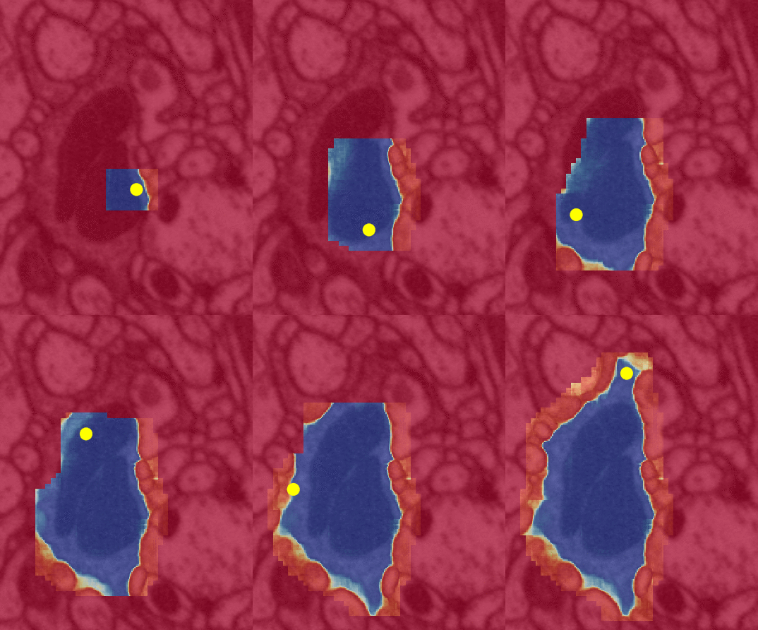
Tracing neurites in large-scale electron microscopy data is an example of an image segmentation problem. Traditional algorithms have divided the process into at least two steps: finding boundaries between neurites using an edge detector or a machine-learning classifier, and then grouping together image pixels that are not separated by a boundary using an algorithm like watershed or graph cut. In 2015, we began experimenting with an alternative approach based on recurrent neural networks that unifies these two steps. The algorithm is seeded at a specific pixel location and then iteratively “fills” a region using a recurrent convolutional neural network that predicts which pixels are part of the same object as the seed. Since 2015, we have been working to apply this new approach to large-scale connectomics datasets and rigorously quantify its accuracy.
A flood-filling network segmenting an object in 2d. The yellow dot is the center of the current area of focus; the algorithm expands the segmented region (blue) as it iteratively examines more of the overall image.
Measuring Accuracy via Expected Run Length
Working with our partners at the Max Planck Institute, we devised a metric we call “expected run length” (ERL) that measures the following: given a random point within a random neuron in a 3d image of a brain, how far can we trace the neuron before making some kind of mistake? This is an example of a mean-time-between-failure metric, except that in this case we measure the amount of space between failures rather than the amount of time. For engineers, the appeal of ERL is that it relates a linear, physical path length to the frequency of individual mistakes that are made by an algorithm, and that it can be computed in a straightforward way. For biologists, the appeal is that a particular numerical value of ERL can be related to biologically relevant quantities, such as the average path length of neurons in different parts of the nervous system.
Progress in expected run length (blue line) leading up to the results shared today in Nature Methods. The red line shows progress in the “merge rate,” which measures the frequency with which two separate neurites were erroneously traced as a single object; achieving a very low merge rate is important for enabling efficient strategies for manual identification and correction of the remaining errors in the reconstruction.
Songbird Connectomics
We used ERL to measure our progress on a ground-truth set of neurons within a 1-million cubic micron zebra finch song-bird brain imaged by our collaborators using serial block-face scanning electron microscopy and found that our approach performed much better than previous deep learning pipelines applied to the same dataset.
Our algorithm in action as it traces a single neurite in 3d in a songbird brain.
We segmented every neuron in a small portion of a zebra finch song-bird brain using the new flood-filling network approach, as depicted here:
Reconstruction of a portion of zebra finch brain. Colors denote distinct objects in the segmentation that was automatically generated using a flood-filling network. Gold spheres represent synaptic locations automatically identified using a previously published approach.
By combining these automated results with a small amount of additional human effort required to fix the remaining errors, our collaborators at the Max Planck Institute are now able to study the songbird connectome to derive new insights into how zebra finch birds sing their song and test theories related to how they learn their song.

Next Steps
We will continue to improve connectomics reconstruction technology, with the aim of fully automating synapse-resolution connectomics and contributing to ongoing connectomics projects at the Max Planck Institute and elsewhere. In order to help support the larger research community in developing connectomics techniques, we have also open-sourced the TensorFlow code for the flood-filling network approach, along with WebGL visualization software for 3d datasets that we developed to help us understand and improve our reconstruction results.

Acknowledgements
We would like to acknowledge core contributions from Tim Blakely, Peter Li, Larry Lindsey, Jeremy Maitin-Shepard, Art Pope and Mike Tyka (Google), as well as Joergen Kornfeld and Winfried Denk (Max Planck Institute).

Source: Google AI Blog


Accelerated Training and Inference with the Tensorflow Object Detection API


Last year we announced the TensorFlow Object Detection API, and since then we’ve released a number of new features, such as models learned via Neural Architecture Search, instance segmentation support and models trained on new datasets such as Open Images. We have been amazed at how it is being used – from finding scofflaws on the streets of NYC to diagnosing diseases on cassava plants in Tanzania.
Today, as part of Google’s commitment to democratizing computer vision, and using feedback from the research community on how to make this codebase even more useful, we’re excited to announce a number of additions to our API. Highlights of this release include:
  • Support for accelerated training of object detection models via Cloud TPUs
  • Improving the mobile deployment process by accelerating inference and making it easy to export a model to mobile with the TensorFlow Lite format
  • Several new model architecture definitions including:
Additionally, we are releasing pre-trained weights for each of the above models based on the COCO dataset.

Accelerated Training via Cloud TPUs
Users spend a great deal of time on optimizing hyperparameters and retraining object detection models, therefore having fast turnaround times on experiments is critical. The models released today belong to the single shot detector (SSD) class of architectures that are optimized for training on Cloud TPUs. For example, we can now train a ResNet-50 based RetinaNet model to achieve 35% mean Average Precision (mAP) on the COCO dataset in < 3.5 hrs.
Accelerated Inference via Quantization and TensorFlow Lite 
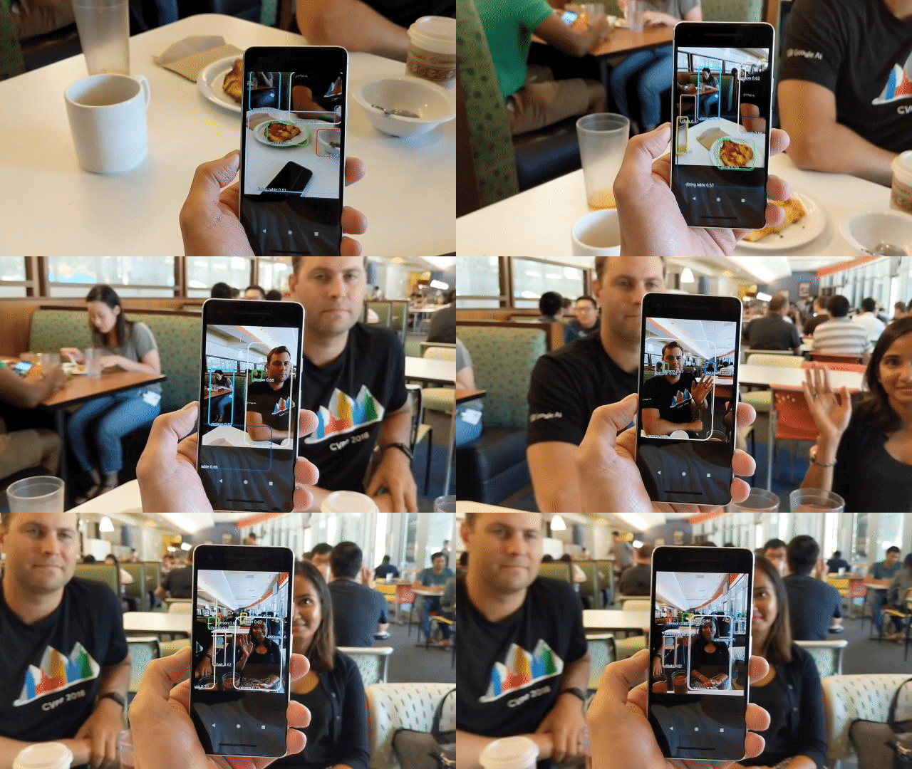
To better support low-latency requirements on mobile and embedded devices, the models we are providing are now natively compatible with TensorFlow Lite, which enables on-device machine learning inference with low latency and a small binary size. As part of this, we have implemented: (1) model quantization and (2) detection-specific operations natively in TensorFlow Lite. Our model quantization follows the strategy outlined in Jacob et al. (2018) and the whitepaper by Krishnamoorthi (2018) which applies quantization to both model weights and activations at training and inference time, yielding smaller models that run faster.
Quantized detection models are faster and smaller (e.g., a quantized 75% depth-reduced SSD Mobilenet model runs at >15 fps on a Pixel 2 CPU with a 4.2 Mb footprint) with minimal loss in detection accuracy compared to the full floating point model.
Try it Yourself with a New Tutorial!
To get started training your own model on Cloud TPUs, check out our new tutorial! This walkthrough will take you through the process of training a quantized pet face detector on Cloud TPU then exporting it to an Android phone for inference via TensorFlow Lite conversion.

We hope that these new additions will help make high-quality computer vision models accessible to anyone wishing to solve an object detection problem, and provide a more seamless user experience, from training a model with quantization to exporting to a TensorFlow Lite model ready for on-device deployment. We would like to thank everyone in the community who have contributed features and bug fixes. As always, contributions to the codebase are welcome, and please stay tuned for more updates!

Acknowledgements
This post reflects the work of the following group of core contributors: Derek Chow, Aakanksha Chowdhery, Jonathan Huang, Pengchong Jin, Zhichao Lu, Vivek Rathod, Ronny Votel and Xiangxin Zhu. We would also like to thank the following colleagues: Vasu Agrawal, Sourabh Bajaj, Chiachen Chou, Tom Jablin, Wenzhe Li, Tsung-Yi Lin, Hernan Moraldo, Kevin Murphy, Sara Robinson, Andrew Selle, Shashi Shekhar, Yash Sonthalia, Zak Stone, Pete Warden and Menglong Zhu.

Source: Google AI Blog