Tag Archives: Computer Vision

EfficientNet: Improving Accuracy and Efficiency through AutoML and Model Scaling

Posted by Mingxing Tan, Staff Software Engineer and Quoc V. Le, Principal Scientist, Google AI

Convolutional neural networks (CNNs) are commonly developed at a fixed resource cost, and then scaled up in order to achieve better accuracy when more resources are made available. For example, ResNet can be scaled up from ResNet-18 to ResNet-200 by increasing the number of layers, and recently, GPipe achieved 84.3% ImageNet top-1 accuracy by scaling up a baseline CNN by a factor of four. The conventional practice for model scaling is to arbitrarily increase the CNN depth or width, or to use larger input image resolution for training and evaluation. While these methods do improve accuracy, they usually require tedious manual tuning, and still often yield suboptimal performance. What if, instead, we could find a more principled method to scale up a CNN to obtain better accuracy and efficiency?

In our ICML 2019 paper, “EfficientNet: Rethinking Model Scaling for Convolutional Neural Networks”, we propose a novel model scaling method that uses a simple yet highly effective compound coefficient to scale up CNNs in a more structured manner. Unlike conventional approaches that arbitrarily scale network dimensions, such as width, depth and resolution, our method uniformly scales each dimension with a fixed set of scaling coefficients. Powered by this novel scaling method and recent progress on AutoML, we have developed a family of models, called EfficientNets, which superpass state-of-the-art accuracy with up to 10x better efficiency (smaller and faster).

Compound Model Scaling: A Better Way to Scale Up CNNs
In order to understand the effect of scaling the network, we systematically studied the impact of scaling different dimensions of the model. While scaling individual dimensions improves model performance, we observed that balancing all dimensions of the network—width, depth, and image resolution—against the available resources would best improve overall performance.

The first step in the compound scaling method is to perform a grid search to find the relationship between different scaling dimensions of the baseline network under a fixed resource constraint (e.g., 2x more FLOPS).This determines the appropriate scaling coefficient for each of the dimensions mentioned above. We then apply those coefficients to scale up the baseline network to the desired target model size or computational budget.

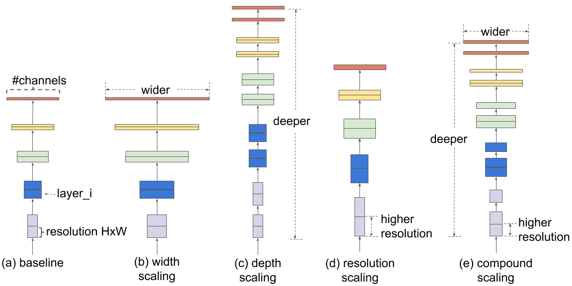
Comparison of different scaling methods. Unlike conventional scaling methods (b)-(d) that arbitrary scale a single dimension of the network, our compound scaling method uniformly scales up all dimensions in a principled way.

This compound scaling method consistently improves model accuracy and efficiency for scaling up existing models such as MobileNet (+1.4% imagenet accuracy), and ResNet (+0.7%), compared to conventional scaling methods.

EfficientNet Architecture
The effectiveness of model scaling also relies heavily on the baseline network. So, to further improve performance, we have also developed a new baseline network by performing a neural architecture search using the AutoML MNAS framework, which optimizes both accuracy and efficiency (FLOPS). The resulting architecture uses mobile inverted bottleneck convolution (MBConv), similar to MobileNetV2 and MnasNet, but is slightly larger due to an increased FLOP budget. We then scale up the baseline network to obtain a family of models, called EfficientNets.

The architecture for our baseline network EfficientNet-B0 is simple and clean, making it easier to scale and generalize.

EfficientNet Performance
We have compared our EfficientNets with other existing CNNs on ImageNet. In general, the EfficientNet models achieve both higher accuracy and better efficiency over existing CNNs, reducing parameter size and FLOPS by an order of magnitude. For example, in the high-accuracy regime, our EfficientNet-B7 reaches state-of-the-art 84.4% top-1 / 97.1% top-5 accuracy on ImageNet, while being 8.4x smaller and 6.1x faster on CPU inference than the previous Gpipe. Compared with the widely used ResNet-50, our EfficientNet-B4 uses similar FLOPS, while improving the top-1 accuracy from 76.3% of ResNet-50 to 82.6% (+6.3%).

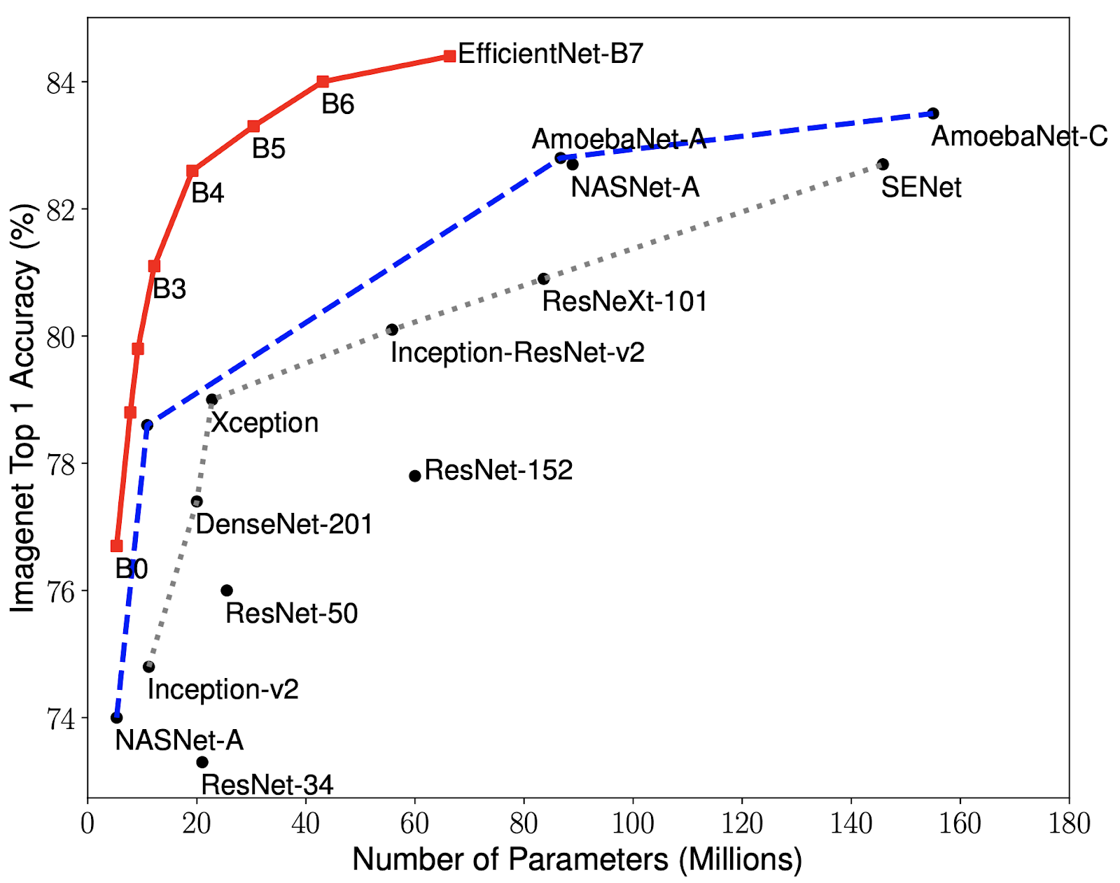
Model Size vs. Accuracy Comparison. EfficientNet-B0 is the baseline network developed by AutoML MNAS, while Efficient-B1 to B7 are obtained by scaling up the baseline network. In particular, our EfficientNet-B7 achieves new state-of-the-art 84.4% top-1 / 97.1% top-5 accuracy, while being 8.4x smaller than the best existing CNN.

Though EfficientNets perform well on ImageNet, to be most useful, they should also transfer to other datasets. To evaluate this, we tested EfficientNets on eight widely used transfer learning datasets. EfficientNets achieved state-of-the-art accuracy in 5 out of the 8 datasets, such as CIFAR-100 (91.7%) and Flowers (98.8%), with an order of magnitude fewer parameters (up to 21x parameter reduction), suggesting that our EfficientNets also transfer well.

By providing significant improvements to model efficiency, we expect EfficientNets could potentially serve as a new foundation for future computer vision tasks. Therefore, we have open-sourced all EfficientNet models, which we hope can benefit the larger machine learning community. You can find the EfficientNet source code and TPU training scripts here.

Acknowledgements:
Special thanks to Hongkun Yu, Ruoming Pang, Vijay Vasudevan, Alok Aggarwal, Barret Zoph, Xianzhi Du, Xiaodan Song, Samy Bengio, Jeff Dean, and the Google Brain team.

Source: Google AI Blog

Moving Camera, Moving People: A Deep Learning Approach to Depth Prediction

Posted by Tali Dekel, Research Scientist and Forrester Cole, Software Engineer, Machine Perception

The human visual system has a remarkable ability to make sense of our 3D world from its 2D projection. Even in complex environments with multiple moving objects, people are able to maintain a feasible interpretation of the objects’ geometry and depth ordering. The field of computer vision has long studied how to achieve similar capabilities by computationally reconstructing a scene’s geometry from 2D image data, but robust reconstruction remains difficult in many cases.

A particularly challenging case occurs when both the camera and the objects in the scene are freely moving. This confuses traditional 3D reconstruction algorithms that are based on triangulation, which assumes that the same object can be observed from at least two different viewpoints, at the same time. Satisfying this assumption requires either a multi-camera array (like Google’s Jump), or a scene that remains stationary as the single camera moves through it. As a result, most existing methods either filter out moving objects (assigning them “zero” depth values), or ignore them (resulting in incorrect depth values).

Left: The traditional stereo setup assumes that at least two viewpoints capture the scene at the same time. Right: We consider the setup where both camera and subject are moving.

In “Learning the Depths of Moving People by Watching Frozen People”, we tackle this fundamental challenge by applying a deep learning-based approach that can generate depth maps from an ordinary video, where both the camera and subjects are freely moving. The model avoids direct 3D triangulation by learning priors on human pose and shape from data. While there is a recent surge in using machine learning for depth prediction, this work is the first to tailor a learning-based approach to the case of simultaneous camera and human motion. In this work, we focus specifically on humans because they are an interesting target for augmented reality and 3D video effects.

Our model predicts the depth map (right; brighter=closer to the camera) from a regular video (left), where both the people in the scene and the camera are freely moving.

Sourcing the Training Data
We train our depth-prediction model in a supervised manner, which requires videos of natural scenes, captured by moving cameras, along with accurate depth maps. The key question is where to get such data. Generating data synthetically requires realistic modeling and rendering of a wide range of scenes and natural human actions, which is challenging. Further, a model trained on such data may have difficulty generalizing to real scenes. Another approach might be to record real scenes with an RGBD sensor (e.g., Microsoft’s Kinect), but depth sensors are typically limited to indoor environments and have their own set of 3D reconstruction issues.

Instead, we make use of an existing source of data for supervision: YouTube videos in which people imitate mannequins by freezing in a wide variety of natural poses, while a hand-held camera tours the scene. Because the entire scene is stationary (only the camera is moving), triangulation-based methods--like multi-view-stereo (MVS)--work, and we can get accurate depth maps for the entire scene including the people in it. We gathered approximately 2000 such videos, spanning a wide range of realistic scenes with people naturally posing in different group configurations.

Videos of people imitating mannequins while a camera tours the scene, which we used for training. We use traditional MVS algorithms to estimate depth, which serves as supervision during training of our depth-prediction model.

Inferring the Depth of Moving People
The Mannequin Challenge videos provide depth supervision for moving camera and “frozen” people, but our goal is to handle videos with a moving camera and moving people. We need to structure the input to the network in order to bridge that gap.

A possible approach is to infer depth separately for each frame of the video (i.e., the input to the model is just a single frame). While such a model already improves over state-of-the-art single image methods for depth prediction, we can improve the results further by considering information from multiple frames. For example, motion parallax, i.e., the relative apparent motion of static objects between two different viewpoints, provides strong depth cues. To benefit from such information, we compute the 2D optical flow between each input frame and another frame in the video, which represents the pixel displacement between the two frames. This flow field depends on both the scene’s depth and the relative position of the camera. However, because the camera positions are known, we can remove their dependency from the flow field, which results in an initial depth map. This initial depth is valid only for static scene regions. To handle moving people at test time, we apply a human-segmentation network to mask out human regions in the initial depth map. The full input to our network then includes: the RGB image, the human mask, and the masked depth map from parallax.

Depth prediction network: The input to the model includes an RGB image (Frame t), a mask of the human region, and an initial depth for the non-human regions, computed from motion parallax (optical flow) between the input frame and another frame in the video. The model outputs a full depth map for Frame t. Supervision for training is provided by the depth map, computed by MVS.

The network’s job is to “inpaint” the depth values for the regions with people, and refine the depth elsewhere. Intuitively, because humans have consistent shape and physical dimensions, the network can internally learn such priors by observing many training examples. Once trained, our model can handle natural videos with arbitrary camera and human motion.

Below are some examples of our depth-prediction model results based on videos, with comparison to recent state-of-the-art learning based methods.

Comparison of depth prediction models to a video clip with moving cameras and people. Top: Learning based monocular depth prediction methods (DORN; Chen et al.). Bottom: Learning based stereo method (DeMoN), and our result.

3D Video Effects Using Our Depth Maps
Our predicted depth maps can be used to produce a range of 3D-aware video effects. One such effect is synthetic defocus. Below is an example, produced from an ordinary video using our depth map.

Bokeh video effect produced using our estimated depth maps. Video courtesy of Wind Walk Travel Videos.

Other possible applications for our depth maps include generating a stereo video from a monocular one, and inserting synthetic CG objects into the scene. Depth maps also provide the ability to fill in holes and disoccluded regions with the content exposed in other frames of the video. In the following example, we have synthetically wiggled the camera at several frames and filled in the regions behind the actor with pixels from other frames of the video.

Acknowledgements
The research described in this post was done by Zhengqi Li, Tali Dekel, Forrester Cole, Richard Tucker, Noah Snavely, Ce Liu and Bill Freeman. We would like to thank Miki Rubinstein for his valuable feedback.

Source: Google AI Blog

Announcing Open Images V5 and the ICCV 2019 Open Images Challenge

Posted by Vittorio Ferrari, Research Scientist, Machine Perception

In 2016, we introduced Open Images, a collaborative release of ~9 million images annotated with labels spanning thousands of object categories. Since then we have rolled out several updates, culminating with Open Images V4 in 2018. In total, that release included 15.4M bounding-boxes for 600 object categories, making it the largest existing dataset with object location annotations, as well as over 300k visual relationship annotations.

Today we are happy to announce Open Images V5, which adds segmentation masks to the set of annotations, along with the second Open Images Challenge, which will feature a new instance segmentation track based on this data.

Open Images V5
Open Images V5 features segmentation masks for 2.8 million object instances in 350 categories. Unlike bounding-boxes, which only identify regions in which an object is located, segmentation masks mark the outline of objects, characterizing their spatial extent to a much higher level of detail. We have put particular effort into ensuring consistent annotations across different objects (e.g., all cat masks include their tail; bags carried by camels or persons are included in their mask). Importantly, these masks cover a broader range of object categories and a larger total number of instances than any previous dataset.

Example masks on the training set of Open Images V5. These have been produced by our interactive segmentation process. The first example also shows a bounding box, for comparison. From left to right, top to bottom: Tea and cake at the Fitzwilliam Museum by Tim Regan, Pilota II by Euskal kultur erakundea Institut culturel basque, Rheas by Dag Peak, Wuxi science park, 1995 by Gary Stevens, Cat Cafe Shinjuku calico by Ari Helminen, and Untitled by Todd Huffman. All images used under CC BY 2.0 license.

The segmentation masks on the training set (2.68M) have been produced by our state-of-the-art interactive segmentation process, where professional human annotators iteratively correct the output of a segmentation neural network. This is more efficient than manual drawing alone, while at the same time delivering accurate masks (intersection-over-union 84%). Additionally, we release 99k masks on the validation and test sets, which have been annotated manually with a strong focus on quality. These are near-perfect and capture even fine details of complex object boundaries (e.g. spiky flowers and thin structures in man-made objects). Both our training and validation+test annotations offer more accurate object boundaries than the polygon annotations provided by most existing datasets.

Example masks on the validation and test sets of Open Images V5, drawn completely manually. From left to right: thistle flowers by sophie, still life with ax by liz west, Fischkutter KOŁ-180 in Kolobrzeg (PL) by zeesenboot. All images used under CC BY 2.0 license.

In addition to the masks, we also added 6.4M new human-verified image-level labels, reaching a total of 36.5M over nearly 20,000 categories. Finally, we improved annotation density for 600 object categories on the validation and test sets, adding more than 400k bounding boxes to match the density in the training set. This ensures more precise evaluation of object detection models.

Open Images Challenge 2019
In conjunction with this release, we are also introducing the second Open Images Challenge, to be held at the 2019 International Conference on Computer Vision (ICCV 2019). This Challenge will have a new instance segmentation track based on the data above. Moreover, as in the 2018 edition, it will also feature a large-scale object detection track (500 categories with 12.2M training bounding-boxes), and a visual relationship detection track for detecting pairs of objects in particular relations (329 relationship triplets with 375k training samples, e.g., “woman playing guitar” or “beer on table”).

The training set with all annotations is available now. The test set has the same 100k images as the 2018 Challenge and will be launched again on June 3rd, 2019 by Kaggle. The evaluation servers will open on June 3rd for the object detection and visual relationship tracks, and on July 1st for the instance segmentation track. The deadline for submission of results is October 1st, 2019.

We hope that the exceptionally large and diverse training set will inspire research into more advanced instance segmentation models. The extremely accurate ground-truth masks we provide rewards subtle improvements in the output segmentations, and thus will encourage the development of higher-quality models that deliver precise boundaries. Finally, having a single dataset with unified annotations for image classification, object detection, visual relationship detection, and instance segmentation will enable researchers to study these tasks jointly and stimulate progress towards genuine scene understanding.

Source: Google AI Blog

Announcing Google-Landmarks-v2: An Improved Dataset for Landmark Recognition & Retrieval

Posted by Bingyi Cao and Tobias Weyand, Software Engineers, Google AI

Last year we released Google-Landmarks, the largest world-wide landmark recognition dataset available at that time. In order to foster advancements in research on instance-level recognition (recognizing specific instances of objects, e.g. distinguishing Niagara Falls from just any waterfall) and image retrieval (matching a specific object in an input image to all other instances of that object in a catalog of reference images), we also hosted two Kaggle challenges, Landmark Recognition 2018 and Landmark Retrieval 2018, in which more than 500 teams of researchers and machine learning (ML) enthusiasts participated. However, both instance recognition and image retrieval methods require ever larger datasets in both the number of images and the variety of landmarks in order to train better and more robust systems.

In support of this goal, this year we are releasing Google-Landmarks-v2, a completely new, even larger landmark recognition dataset that includes over 5 million images (2x that of the first release) of more than 200 thousand different landmarks (an increase of 7x). Due to the difference in scale, this dataset is much more diverse and creates even greater challenges for state-of-the-art instance recognition approaches. Based on this new dataset, we are also announcing two new Kaggle challenges—Landmark Recognition 2019 and Landmark Retrieval 2019—and releasing the source code and model for Detect-to-Retrieve, a novel image representation suitable for retrieval of specific object instances.

Heatmap of the landmark locations in Google-Landmarks-v2, which demonstrates the increase in the scale of the dataset and the improved geographic coverage compared to last year’s dataset.

Creating the Dataset
A particular problem in preparing Google-Landmarks-v2 was the generation of instance labels for the landmarks represented, since it is virtually impossible for annotators to recognize all of the hundreds of thousands of landmarks that could potentially be present in a given photo. Our solution to this problem was to crowdsource the landmark labeling through the efforts of a world-spanning community of hobby photographers, each familiar with the landmarks in their region.

Selection of images from Google-Landmarks-v2. Landmarks include (left to right, top to bottom) Neuschwanstein Castle, Golden Gate Bridge, Kiyomizu-dera, Burj khalifa, Great Sphinx of Giza, and Machu Picchu.

Another issue for research datasets is the requirement that images be shared freely and stored indefinitely, so that the dataset can be used to track the progress of research over a long period of time. As such, we sourced the Google-Landmarks-v2 images through Wikimedia Commons, capturing both world-famous and lesser-known, local landmarks while ensuring broad geographic coverage (thanks in part to Wiki Loves Monuments) and photos sourced from public institutions, including historical photographs that are valuable to test instance recognition over time.

The Kaggle Challenges
The goal of the Landmark Recognition 2019 challenge is to recognize a landmark presented in a query image, while the goal of Landmark Retrieval 2019 is to find all images showing that landmark. The challenges include cash prizes totaling $50,000 and the winning teams will be invited to present their methods at the Second Landmark Recognition Workshop at CVPR 2019.

Open Sourcing our Model
To foster research reproducibility and help push the field of instance recognition forward, we are also releasing open-source code for our new technique, called Detect-to-Retrieve (which will be presented as a paper in CVPR 2019). This new method leverages bounding boxes from an object detection model to give extra weight to image regions containing the class of interest, which significantly improves accuracy. The model we are releasing is trained on a subset of 86k images from the original Google-Landmarks dataset that were annotated with landmark bounding boxes. We are making these annotations available along with the original dataset here.

We invite researchers and ML enthusiasts to participate in the Landmark Recognition 2019 and Landmark Retrieval 2019 Kaggle challenges and to join the Second Landmark Recognition Workshop at CVPR 2019. We hope that this dataset will help advance the state-of-the-art in instance recognition and image retrieval. The data is being made available via the Common Visual Data Foundation.

Acknowledgments
The core contributors to this project are Andre Araujo, Bingyi Cao, Jack Sim and Tobias Weyand. We would like to thank our team members Daniel Kim, Emily Manoogian, Nicole Maffeo, and Hartwig Adam for their kind help. Thanks also to Marvin Teichmann and Menglong Zhu for their contribution to collecting the landmark bounding boxes and developing the Detect-to-Retrieve technique. We would like to thank Will Cukierski and Maggie Demkin for their help organizing the Kaggle challenge, Elan Hourticolon-Retzler, Yuan Gao, Qin Guo, Gang Huang, Yan Wang, Zhicheng Zheng for their help with data collection, Tsung-Yi Lin for his support with CVDF hosting, as well as our CVPR workshop co-organizers Bohyung Han, Shih-Fu Chang, Ondrej Chum, Torsten Sattler, Giorgos Tolias, and Xu Zhang. We have great appreciation for the Wikimedia Commons Community and their volunteer contributions to an invaluable photographic archive of the world’s cultural heritage. And finally, we’d like to thank the Common Visual Data Foundation for hosting the dataset.

Source: Google AI Blog

Announcing the 6th Fine-Grained Visual Categorization Workshop

Posted by Christine Kaeser-Chen, Software Engineer and Serge Belongie, Visiting Faculty, Google AI

In recent years, fine-grained visual recognition competitions (FGVCs), such as the iNaturalist species classification challenge and the iMaterialist product attribute recognition challenge, have spurred progress in the development of image classification models focused on detection of fine-grained visual details in both natural and man-made objects. Whereas traditional image classification competitions focus on distinguishing generic categories (e.g., car vs. butterfly), the FGVCs go beyond entry level categories to focus on subtle differences in object parts and attributes. For example, rather than pursuing methods that can distinguish categories, such as “bird”, we are interested in identifying subcategories such as “indigo bunting” or “lazuli bunting.”

Previous challenges attracted a large number of talented participants who developed innovative new models for image recognition, with more than 500 teams competing at FGVC5 at CVPR 2018. FGVC challenges have also inspired new methods such as domain-specific transfer learning and estimating test-time priors, which have helped fine-grained recognition tasks reach state-of-the-art performance on several benchmarking datasets.

In order to further spur progress in FGVC research, we are proud to sponsor and co-organize the 6th annual workshop on Fine-Grained Visual Categorization (FGVC6), to be held on June 17th in Long Beach, CA at CVPR 2019. This workshop brings together experts in computer vision with specialists focusing on biodiversity, botany, fashion, and the arts, to address the challenges of applying fine-grained visual categorization to real-life settings.

This Year’s Challenges
This year there will be a wide variety of competition topics, each highlighting unique challenges of fine-grained visual categorization, including an updated iNaturalist challenge, fashion & products, wildlife camera traps, food, butterflies & moths, fashion design, and cassava leaf disease. We are also delighted to introduce two new partnerships with world class institutions—The Metropolitan Museum of Art for the iMet Collection challenge and the New York Botanical Garden for the Herbarium challenge.

The FGVC workshop at CVPR focuses on subordinate categories, including (from left to right, top to bottom) animal species from wildlife camera traps, retail products, fashion attributes, cassava leaf disease, Melastomataceae species from herbarium sheets, animal species from citizen science photos, butterfly and moth species, cuisine of dishes, and fine-grained attributes for museum art objects.

In the iMet Collection challenge, participants compete to train models on artistic attributes including object presence, culture, content, theme, and geographic origin. The Metropolitan Museum of Art provided a large training dataset for this task based on subject matter experts’ descriptions of their museum collections. This dataset highlights the challenge of inferring fine-grained attributes that are grounded in the visual context indirectly (e.g., period, culture, medium).

A diverse sample of images included in the iMet Collection challenge dataset. Images were taken from the Metropolitan Museum of Art’s public domain dataset.

The iMet Collection challenge is also noteworthy for its status as the first image-based Kernels-only competition, a recently introduced option on Kaggle that levels the playing field for data scientists who might not otherwise have access to adequate computational resources. Kernel competitions provide all participants with the same hardware allowances, giving rise to a more balanced competition. Moreover, the winning models tend to be simpler than their counterparts in other competitions, since the participants must work within the compute constraints imposed by the Kernels platform. At the time of writing, the iMet Collection challenge has over 250 participating teams.

In the Herbarium challenge, researchers are invited to tackle the problem of classifying species from the flowering plant family Melastomataceae. This challenge is distinguished from the iNaturalist competition, since the included images depict dried specimens preserved on herbarium sheets, exclusively. Herbarium sheets are essential to plant science, as they not only preserve the key details of the plants for identification and DNA analysis, but also provide a rare perspective into plant ecology in a historical context. As the world’s second largest herbarium, NYBG’s Steere Herbarium collection contributed a dataset of over 46,000 specimens for this year’s challenge.

In the Herbarium challenge, participants will identify species from the flowering plant family Melastomataceae. The New York Botanical Garden (NYBG) provided a dataset of over 46,000 herbarium specimens including over 680 species. Images used with permission of the NYBG.

Every one of this year’s challenges requires deep engagement with subject matter experts, in addition to institutional coordination. By teeing up image recognition challenges in a standard format, the FGVC workshop paves the way for technology transfer from the top of the Kaggle leaderboards into the hands of everyday users via mobile apps such as Seek by iNaturalist and Merlin Bird ID. We anticipate the techniques developed by our competition participants will not only push the frontier of fine-grained recognition, but also be beneficial for applying machine vision to advance scientific exploration and curatorial studies.

Invitation to Participate
We invite teams to participate in these competitions to help advance the state-of-the-art in fine-grained image recognition. Deadlines for entry into the competitions range from May 26 to June 3, depending on the challenge. The results of these competitions will be presented at the FGVC6 workshop at CVPR 2019, and will provide broad exposure to the top performing teams. We are excited to encourage the community's development of more accurate and broadly impactful algorithms in the field of fine-grained visual categorization!

Acknowledgements
We’d like to thank our colleagues and friends on the FGVC6 organizing committee for working together to advance this important area. At Google we would like to thank Hartwig Adam, Chenyang Zhang, Yulong Liu, Kiat Chuan Tan, Mikhail Sirotenko, Denis Brulé, Cédric Deltheil, Timnit Gebru, Ernest Mwebaze, Weijun Wang, Grace Chu, Jack Sim, Andrew Howard, R.V. Guha, Srikanth Belwadi, Tanya Birch, Katherine Chou, Maggie Demkin, Elizabeth Park, and Will Cukierski.

Source: Google AI Blog

Take Your Best Selfie Automatically, with Photobooth on Pixel 3

Posted by Navid Shiee, Senior Software Engineer and Aseem Agarwala, Staff Research Scientist, Google AI

Taking a good group selfie can be tricky—you need to hover your finger above the shutter, keep everyone’s faces in the frame, look at the camera, make good expressions, try not to shake the camera and hope no one blinks when you finally press the shutter! After building the technology behind automatic photography with Google Clips, we asked ourselves: can we bring some of the magic of this automatic picture experience to the Pixel phone?

With Photobooth, a new shutter-free mode in the Pixel 3 Camera app, it’s now easier to shoot selfies—solo, couples, or even groups—that capture you at your best. Once you enter Photobooth mode and click the shutter button, it will automatically take a photo when the camera is steady and it sees that the subjects have good expressions with their eyes open. And in the newest release of Pixel Camera, we’ve added kiss detection to Photobooth! Kiss a loved one, and the camera will automatically capture it.

Photobooth automatically captures group shots, when everyone in the photo looks their best.

Photobooth joins Top Shot and Portrait mode in a suite of exciting Pixel camera features that enable you to take the best pictures possible. However, unlike Portrait mode, which takes advantage of specialized hardware in the back-facing camera to provide its most accurate results, Photobooth is optimized for the front-facing camera. To build Photobooth, we had to solve for three challenges: how to identify good content for a wide range of user groups; how to time the shutter to capture the best moment; and how to animate a visual element that helps users understand what Photobooth sees and captures.

Models for Understanding Good Content
In developing Photobooth, a main challenge was to determine when there was good content in either a typical selfie, in which the subjects are all looking at the camera, or in a shot that includes people kissing and not necessarily facing the camera. To accomplish this, Photobooth relies on two distinct models to capture good selfies—a model for facial expressions and a model to detect when people kiss.

We worked with photographers to identify five key expressions that should trigger capture: smiles, tongue-out, kissy/duck face, puffy-cheeks, and surprise. We then trained a neural network to classify these expressions. The kiss detection model used by Photobooth is a variation of the Image Content Model (ICM) trained for Google Clips, fine tuned specifically to focus on kissing. Both of these models use MobileNets in order to run efficiently on-device while continuously processing the images at high frame rate. The outputs of the models are used to evaluate the quality of each frame for the shutter control algorithm.

Shutter Control
Once you click the shutter button in Photobooth mode, a basic quality assessment based on the content score from the models above is performed. This first stage is used as a filter that avoids moments that either contain closed eyes, talking, or motion blur, or fail to detect the facial expressions or kissing actions learned by the models. Photobooth temporally analyzes the expression confidence values to detect their presence in the photo, making it robust to variations in the output of machine learning (ML) models. Once the first stage is successfully passed, each frame is subjected to a more fine-grained analysis, which outputs an overall frame score.

The frame score considers both facial expression quality and the kiss score. As the kiss detection model operates on the entire frame, its output can be used directly as a full-frame score value for kissing. The face expressions model outputs a score for each identified expression. Since a variable number of faces may be present in each frame, Photobooth applies an attention model using the detected expressions to iteratively compute an expression quality representation and weight for each face. The weighting is important, for example, to emphasize the expressions in the foreground, rather than the background. The model then calculates a single, global score for the quality of expressions in the frame.

The final image quality score used for triggering the shutter is computed by a weighted combination of the attention based facial expression score and the kiss score. In order to detect the peak quality, the shutter control algorithm maintains a short buffer of observed frames and only saves a shot if its frame score is higher than the frames that come after it in the buffer. The length of the buffer is short enough to give users a sense of real time feedback.

Intelligence Indicator
Since Photobooth uses the front-facing camera, the user can see and interact with the display while taking a photo. Photobooth mode includes a visual indicator, a bar at the top of the screen that grows in size when photo quality scores increase, to help users understand what the ML algorithms see and capture. The length of the bar is divided into four distinct ranges: (1) no faces clearly seen, (2) faces seen but not paying attention to the camera, (3) faces paying attention but not making key expressions, and (4) faces paying attention with key expressions.

In order to make this indicator more interpretable, we forced the bar into these ranges, which prevented the bar scaling from being too rapid. This resulted in smooth variability of the bar length as the quality score changes and improved the utility. When the indicator bar reaches a length representative of a high quality score, the screen flashes to signify that a photo was captured and saved.

Using ML outputs directly as intelligence feedback results in rapid variation (left), whereas specifying explicit ranges creates a smooth signal (right).

Conclusion
We’re excited by the possibilities of automatic photography on camera phones. As computer vision continues to improve, in the future we may generally trust smart cameras to select a great moment to capture. Photobooth is an example of how we can carve out a useful corner of this space—selfies and group selfies of smiles, funny faces, and kisses—and deliver a fun and useful experience.

Acknowledgments
Photobooth was a collaboration of several teams at Google. Key contributors to the project include: Kojo Acquah, Chris Breithaupt, Chun-Te Chu, Geoff Clark, Laura Culp, Aaron Donsbach, Relja Ivanovic, Pooja Jhunjhunwala, Xuhui Jia, Ting Liu, Arjun Narayanan, Eric Penner, Arushan Raj, Divya Tyam, Raviteja Vemulapalli, Julian Walker, Jun Xie, Li Zhang, Andrey Zhmoginov, Yukun Zhu.

Source: Google AI Blog

Capturing Special Video Moments with Google Photos

Posted by Sudheendra Vijayanarasimhan and David Ross, Software Engineers

Recording video of memorable moments to share with friends and loved ones has become commonplace. But as anyone with a sizable video library can tell you, it's a time consuming task to go through all that raw footage searching for the perfect clips to relive or share with family and friends. Google Photos makes this easier by automatically finding magical moments in your videos—like when your child blows out the candle or when your friend jumps into a pool—and creating animations from them that you can easily share with friends and family.

In "Rethinking the Faster R-CNN Architecture for Temporal Action Localization", we address some of the challenges behind automating this task, which are due to the complexity of identifying and categorizing actions from a highly variable array of input data, by introducing an improved method to identify the exact location within a video where a given action occurs. Our temporal action localization network (TALNet) draws inspiration from advances in region-based object detection methods such as the Faster R-CNN network. TALNet enables identification of moments with large variation in duration, achieving state-of-the-art performance compared to other methods, allowing Google Photos to recommend the best part of a video for you to share with friends and family.

An example of the detected action "blowing out candles"

Identifying Actions for Model Training
The first step in identifying magic moments in videos is to assemble a list of actions that people might wish to highlight. Some examples of actions include "blow out birthday candles", "strike (bowling)", "cat wags tail", etc. We then crowdsourced the annotation of segments within a collection of public videos where these specific actions occurred, in order to create a large training dataset. We asked the raters to find and label all moments, accommodating videos that might have several moments. This final annotated dataset was then used to train our model so that it could identify the desired actions in new, unknown videos.

Comparison to Object Detection
The challenge of recognizing these actions belongs to the field of computer vision known as temporal action localization, which, like the more familiar object detection, falls under the umbrella of visual detection problems. Given a long, untrimmed video as input, temporal action localization aims to identify the start and end times, as well as the action label (like "blowing out candles"), for each action instance in the full video. While object detection aims to produce spatial bounding boxes around an object in a 2D image, temporal action localization aims to produce temporal segments including an action in a 1D sequence of video frames.

Our approach to TALNet is inspired by the faster R-CNN object detection framework for 2D images. So, to understand TALNet, it is useful to first understand faster R-CNN. The figure below demonstrates how the faster R-CNN architecture is used for object detection. The first step is to generate a set of object proposals, regions of the image that can be used for classification. To do this, an input image is first converted into a 2D feature map by a convolutional neural network (CNN). The region proposal network then generates bounding boxes around candidate objects. These boxes are generated at multiple scales in order to capture the large variability in objects' sizes in natural images. With the object proposals now defined, the subjects in the bounding boxes are then classified by a deep neural network (DNN) into specific objects, such as "person", "bike", etc.

Faster R-CNN architecture for object detection

Temporal Action Localization
Temporal action localization is accomplished in a fashion similar to that used by R-CNN. A sequence of input frames from a video are first converted into a sequence of 1D feature maps that encode scene context. This map is passed to a segment proposal network that generates candidate segments, each defined by start and end times. A DNN then applies the representations learned from the training dataset to classify the actions in the proposed video segments (e.g., "slam dunk", "pass", etc.). The actions identified in each segment are given weights according to their learned representations, with the top scoring moment selected to share with the user.

Architecture for temporal action localization

Special Considerations for Temporal Action Localization
While temporal action localization can be viewed as the 1D counterpart of the object detection problem, care must be taken to address a number of issues unique to action localization. In particular, we address three specific issues in order to apply the Faster R-CNN approach to the action localization domain, and redesign the architecture to specifically address them.

Actions have much larger variations in durations
The temporal extent of actions varies dramatically—from a fraction of a second to minutes. For long actions, it is not important to understand each and every frame of the action. Instead, we can get a better handle on the action by skimming quickly through the video, using dilated temporal convolutions. This approach allows TALNet to search the video for temporal patterns, while skipping over alternate frames based on a given dilation rate. Analysing the video with several different rates that are selected automatically according to the anchor segment's length enables efficient identification of actions as large as the entire video or as short as a second.
The context before and after an action are important
The moments preceding and following an action instance contain critical information for localization and classification, arguably more so than the spatial context of an object. Therefore, we explicitly encode the temporal context by extending the length of proposal segments on both the left and right by a fixed percentage of the segment's length in both the proposal generation stage and the classification stage.
Actions require multi-modal input
Actions are defined by appearance, motion and sometimes even audio information. Therefore, it is important to consider multiple modalities of features for the best results. We use a late fusion scheme for both the proposal generation network and the classification network, in which each modality has a separate proposal generation network whose outputs are combined together to obtain the final set of proposals. These proposals are classified using separate classification networks for each modality, which are then averaged to obtain the final predictions.

TALNet in Action
As a consequence of these improvements, TALNet achieves state-of-the-art performance for both action proposal and action localization tasks on the THUMOS'14 detection benchmark and competitive performance on the ActivityNet challenge. Now, whenever people save videos to Google Photos, our model identifies these moments and creates animations to share. Here are a few examples shared by our initial testers.

An example of the detected action "sliding down a slide"

An example of the detected actions "jump into the pool" (left), "twirl in a dress" (center) and "feed baby a spoonful" (right).

Next steps
We are continuing work to improve the precision and recall of action localization using more data, features and models. Improvements in temporal action localization can drive progress on a large number of important topics ranging from video highlights, video summarization, search and more. We hope to continue improving the state-of-the-art in this domain and at the same time provide more ways for people to reminisce on their memories, big and small.

Acknowledgements
Special thanks Tim Novikoff and Yu-Wei Chao, as well as Bryan Seybold, Lily Kharevych, Siyu Gu, Tracy Gu, Tracy Utley, Yael Marzan, Jingyu Cui, Balakrishnan Varadarajan, Paul Natsev for their critical contributions to this project.

Source: Google AI Blog

Real-Time AR Self-Expression with Machine Learning

Posted by Artsiom Ablavatski and Ivan Grishchenko, Research Engineers, Google AI

Augmented reality (AR) helps you do more with what you see by overlaying digital content and information on top of the physical world. For example, AR features coming to Google Maps will let you find your way with directions overlaid on top of your real world. With Playground - a creative mode in the Pixel camera -- you can use AR to see the world differently. And with the latest release of YouTube Stories and ARCore's new Augmented Faces API you can add objects like animated masks, glasses, 3D hats and more to your own selfies!

One of the key challenges in making these AR features possible is proper anchoring of the virtual content to the real world; a process that requires a unique set of perceptive technologies able to track the highly dynamic surface geometry across every smile, frown or smirk.

Our 3D mesh and some of the effects it enables

To make all this possible, we employ machine learning (ML) to infer approximate 3D surface geometry to enable visual effects, requiring only a single camera input without the need for a dedicated depth sensor. This approach provides the use of AR effects at realtime speeds, using TensorFlow Lite for mobile CPU inference or its new mobile GPU functionality where available. This technology is the same as what powers YouTube Stories' new creator effects, and is also available to the broader developer community via the latest ARCore SDK release and the ML Kit Face Contour Detection API.

An ML Pipeline for Selfie AR
Our ML pipeline consists of two real-time deep neural network models that work together: A detector that operates on the full image and computes face locations, and a generic 3D mesh model that operates on those locations and predicts the approximate surface geometry via regression. Having the face accurately cropped drastically reduces the need for common data augmentations like affine transformations consisting of rotations, translation and scale changes. Instead it allows the network to dedicate most of its capacity towards coordinate prediction accuracy, which is critical to achieve proper anchoring of the virtual content.

Once the location of interest is cropped, the mesh network is only applied to a single frame at a time, using a windowed smoothing in order to reduce noise when the face is static while avoiding lagging during significant movement.

Our 3D mesh in action

For our 3D mesh we employed transfer learning and trained a network with several objectives: the network simultaneously predicts 3D mesh coordinates on synthetic, rendered data and 2D semantic contours on annotated, real world data similar to those MLKit provides. The resulting network provided us with reasonable 3D mesh predictions not just on synthetic but also on real world data. All models are trained on data sourced from a geographically diverse dataset and subsequently tested on a balanced, diverse testset for qualitative and quantitative performance.

The 3D mesh network receives as input a cropped video frame. It doesn't rely on additional depth input, so it can also be applied to pre-recorded videos. The model outputs the positions of the 3D points, as well as the probability of a face being present and reasonably aligned in the input. A common alternative approach is to predict a 2D heatmap for each landmark, but it is not amenable to depth prediction and has high computational costs for so many points.

We further improve the accuracy and robustness of our model by iteratively bootstrapping and refining predictions. That way we can grow our dataset to increasingly challenging cases, such as grimaces, oblique angle and occlusions. Dataset augmentation techniques also expanded the available ground truth data, developing model resilience to artifacts like camera imperfections or extreme lighting conditions.

Dataset expansion and improvement pipeline

Hardware-tailored Inference
We use TensorFlow Lite for on-device neural network inference. The newly introduced GPU back-end acceleration boosts performance where available, and significantly lowers the power consumption. Furthermore, to cover a wide range of consumer hardware, we designed a variety of model architectures with different performance and efficiency characteristics. The most important differences of the lighter networks are the residual block layout and the accepted input resolution (128x128 pixels in the lightest model vs. 256x256 in the most complex). We also vary the number of layers and the subsampling rate (how fast the input resolution decreases with network depth).

Inference time per frame: CPU vs. GPU

The result of these optimizations is a substantial speedup from using lighter models, with minimal degradation in AR effect quality.

Comparison of the most complex (left) and the lightest models (right). Temporal consistency as well as lip and eye tracking is slightly degraded on light models.

The end result of these efforts empowers a user experience with convincing, realistic selfie AR effects in YouTube, ARCore, and other clients by:

Simulating light reflections via environmental mapping for realistic rendering of glasses
Natural lighting by casting virtual object shadows onto the face mesh
Modelling face occlusions to hide virtual object parts behind a face, e.g. virtual glasses, as shown below.

YouTube Stories includes Creator Effects like realistic virtual glasses, based on our 3D mesh

In addition, we achieve highly realistic makeup effects by:

Modelling Specular reflections applied on lips and
Face painting by using luminance-aware material

Case study comparing real make-up against our AR make-up on 5 subjects under different lighting conditions.

We are excited to share this new technology with creators, users and developers alike, who can use this new technology immediately by downloading the latest ARCore SDK. In the future we plan to broaden this technology to more Google products.

Acknowledgements
We would like to thank Yury Kartynnik, Valentin Bazarevsky, Andrey Vakunov, Siargey Pisarchyk, Andrei Tkachenka, and Matthias Grundmann for collaboration on developing the current mesh technology; Nick Dufour, Avneesh Sud and Chris Bregler for an earlier version of the technology based on parametric models; Kanstantsin Sokal, Matsvei Zhdanovich, Gregory Karpiak, Alexander Kanaukou, Suril Shah, Buck Bourdon, Camillo Lugaresi, Siarhei Kazakou and Igor Kibalchich for building the ML pipeline to drive impressive effects; Aleksandra Volf and the annotation team for their diligence and dedication to perfection; Andrei Kulik, Juhyun Lee, Raman Sarokin, Ekaterina Ignasheva, Nikolay Chirkov, and Yury Pisarchyk for careful benchmarking and insights on mobile GPU-centric network architecture optimizations.

Source: Google AI Blog

Exploring Neural Networks with Activation Atlases

Posted by Shan Carter, Software Engineer, Google AI

Neural networks have become the de facto standard for image-related tasks in computing, currently being deployed in a multitude of scenarios, ranging from automatically tagging photos in your image library to autonomous driving systems. These machine-learned systems have become ubiquitous because they perform more accurately than any system humans were able to directly design without machine learning. But because essential details of these systems are learned during the automated training process, understanding how a network goes about its given task can sometimes remain a bit of a mystery.

Today, in collaboration with colleagues at OpenAI, we're publishing "Exploring Neural Networks with Activation Atlases", which describes a new technique aimed at helping to answer the question of what image classification neural networks "see" when provided an image. Activation atlases provide a new way to peer into convolutional vision networks, giving a global, hierarchical, and human-interpretable overview of concepts within the hidden layers of a network. We think of activation atlases as revealing a machine-learned alphabet for images — an array of simple, atomic concepts that are combined and recombined to form much more complex visual ideas. We are also releasing some jupyter notebooks to help you get you started in making your own activation atlases.

A detail view of an activation atlas from one of the layers of the InceptionV1 vision classification network. It reveals many of the visual detectors that the network uses to classify images, such as different types of fruit-like textures, honeycomb patterns and fabric-like textures.

The activation atlases shown below are built from a convolutional image classification network, Inceptionv1, that was trained on the ImageNet dataset. In general, classification networks are shown an image and then asked to give that image a label from one of 1,000 predetermined classes — such as "carbonara", "snorkel" or "frying pan". To do this, our network evaluates the image data progressively through about ten layers, each made of hundreds of neurons that each activate to varying degrees on different types of image patches. One neuron at one layer might respond positively to a dog's ear, another at an earlier layer might respond to a high-contrast vertical line.

An activation atlas is built by collecting the internal activations from each of these layers of our neural network from one million images. These activations, represented by a complex set of high-dimensional vectors, is projected into useful 2D layouts via UMAP, a dimensionality-reduction technique that preserving some of the local structure of the original high-dimensional space.

This takes care of organizing our activation vectors, but we also need to aggregate them into a more manageable number — all the activations are too many to consume at a glance. To do this, we draw a grid over the 2D layout we created. For each cell in our grid, we average all the activations that lie within the boundaries of that cell, and use feature visualization to create an iconic representation.

Left: A randomized set of one million images is fed through the network, collecting one random spatial activation per image. Center: The activations are fed through UMAP to reduce them to two dimensions. They are then plotted, with similar activations placed near each other. Right: We then draw a grid, average the activations that fall within a cell, and run feature inversion on the averaged activation.

Below we can see an activation atlas for just one layer in a neural network (remember that these classification models can have half a dozen or more layers). It reveals a universe of the visual concepts the network has learned to classify images at this layer. This atlas can be a bit overwhelming at first glance — there's a lot going on! This diversity is a reflection of the variety of visual abstractions and concepts the model has developed.

An overview of an activation atlas for one of the many layers (mixed4c) within Inception v1. It is about halfway through the network.

In this detail, we can see detectors for different types of leaves and plants.

Here we can see different detectors for water, lakes and sandbars.

Here we see different types of buildings and bridges.

As we mentioned before, there are many more layers in this network. Let's look at the layers that came before this one to see how these concepts become more refined as we go deeper into the network (Each layer builds its activations on top of the preceding layer's activations).

In an early layer, mixed4a, there is a vague "mammalian" area.

By the next layer in the network, mixed4b, animals and people have been disentangled, with some fruit and food emerging in the middle.

By layer mixed4c these concepts are further refined and differentiated into small "peninsulas".

Here we've seen the global structure evolve from layer to layer, but each of the individual concepts also become more specific and complex from layer to layer. If we focus on the areas of three layers that contribute to a specific classification, say "cabbage", we can see this clearly.

Left: This early layer is very nonspecific in comparison to the others. Center: By the middle layer, the images definitely resemble leaves, but they could be any type of plant. Right: By the last layer the images are very specific to cabbage, leaves curved into rounded balls.

There is another phenomenon worth noting: not only are concepts being refined as you move from layer to layer, but new concepts seem to be appearing out of combinations of old ones.

You can see how sand and water are distinct concepts in a middle layer, mixed4c (left and center), both with strong attributions to the classification of "sandbar". Contrast this with a later layer (right), mixed5b, where the two ideas seem to be fused into one activation.

Instead of zooming in on certain areas of the whole atlas for a specific layer, we can also create an atlas at a specific layer for just one of the 1,000 classes in ImageNet. This will show the concepts and detectors that the network most often uses to classify a specific class, say "red fox" for instance.

Here we can more clearly see what the network is focusing on to classify a "red fox". There are pointy ears, white snouts surrounded by red fur, and wooded or snowy backgrounds.

Here we can see the many different scales and angles of detectors for "tile roof".

For "ibex", we see detectors for horns and brown fur, but also environments where we might find such animals, like rocky hillsides.

Like the detectors for tile roof, "artichoke" also has many different sizes of detectors for the texture of an artichoke, but we also get some purple flower detectors. These are presumably detecting the blossoms of an artichoke plant.

These atlases not only reveal nuanced visual abstractions within a model, but they can also reveal high-level misunderstandings. For example, by looking at an activation atlas for a "great white shark" we water and triangular fins (as expected) but we also see something that looks like a baseball. This hints at a shortcut taken by this research model where it conflates the red baseball stitching with the open mouth of a great white shark.

We can test this by using a patch of an image of a baseball to switch the model's classification of a particular image from "grey whale" to "great white shark".

We hope that activation atlases will be a useful tool in the quiver of techniques that are making machine learning more accessible and interpretable. To help you get started, we've released several jupyter notebooks which can be executed immediately in your browser with one click via colab. They build upon the previously released toolkit Lucid, which includes code for many other interpretability visualization techniques included as well. We're excited to see what you discover!