Tag Archives: Computer Vision

A New Workflow for Collaborative Machine Learning Research in Biodiversity


The promise of machine learning (ML) for species identification is coming to fruition, revealing its transformative potential in biodiversity research. International workshops such as FGVC and LifeCLEF feature competitions to develop top performing classification algorithms for everything from wildlife camera trap images to pressed flower specimens on herbarium sheets. The encouraging results that have emerged from these competitions inspired us to expand the availability of biodiversity datasets and ML models from workshop-scale to global-scale.

Bringing powerful ML algorithms to the communities that need them requires more than the traditional “big data + big compute” equation. Institutions ranging from natural history museums to citizen science groups take great care to collect and annotate datasets, and the data they share have enabled numerous scientific research publications. But central to the tradition of scholarly research are the conventions of citation and attribution, and it follows that as ML extends its reach into the life sciences, it should bring with it appropriate counterparts to those conventions. More broadly, there is a growing awareness of the importance of ethics, fairness, and transparency within the ML community. As institutions develop and deploy applications of ML at scale, it is critical that they be designed with these considerations in mind.

This week at Biodiversity Next, in collaboration with the Global Biodiversity Information Facility (GBIF), iNaturalist, and Visipedia, we are announcing a new workflow for biodiversity research institutions who would like to make use of ML. With its billion+ species occurrence count contributed by thousands of institutions around the globe, GBIF is playing a vital role in enabling this workflow, whether in terms of data aggregation, collaboration across teams, or standardizing citation practices. In the short term, the most important role relates to an emerging cultural shift in accepted practices for the use of mediated data for training of ML models. In the process of data mediation, GBIF helps ensure that training datasets for ML follow standardized licensing terms, use compatible taxonomies and data formats, and provide fair and sufficient data coverage for the ML task at hand by potentially sampling from multiple source datasets.

This new workflow comprises the following two components:
  1. To assist in developing and refining machine vision models, GBIF will package datasets, taking care to ensure license and citation practice are respected. The training datasets will be issued a Digital Object Identifier (DOI), and will be linked through the DOI citation graph.
  2. To assist application developers, Google and Visipedia will train and publish publicly accessible models with documentation on TensorFlow Hub. These models can then, in turn, be deployed in biodiversity research and citizen science efforts.
Case Study: Recognizing Fungi Species from Photos with the Interactive Mushroom Recognizer
As an illustration of the above workflow, we present an example of fungi recognition. The dataset in this case is curated by the Danish Mycological Society, and formatted, packaged, and shared by GBIF. The dataset provenance, model architecture, license information, and more can be found on the TF Hub model page, along with a live, interactive demonstration of the model that can run on user-supplied images.
Illustration of live, interactive Mushroom Recognizer, powered by a publicly available model trained on a fungi dataset provided by the Danish Mycological Society.
Invitation to Participate
For more information about this initiative, please visit the project page at GBIF. We look forward to engaging with institutions around the globe to enable new and innovative uses of ML for biodiversity.

Acknowledgements
We’d like to thank our collaborators at GBIF, iNaturalist, and Visipedia for working together to develop this workflow. At Google we would like to thank Christine Kaeser-Chen, Chenyang Zhang, Yulong Liu, Kiat Chuan Tan, Christy Cui, Arvi Gjoka, Denis Brulé, Cédric Deltheil, Clément Beauseigneur, Grace Chu, Andrew Howard, Sara Beery, and Katherine Chou.

Source: Google AI Blog


Video Architecture Search

Video understanding is a challenging problem. Because a video contains spatio-temporal data, its feature representation is required to abstract both appearance and motion information. This is not only essential for automated understanding of the semantic content of videos, such as web-video classification or sport activity recognition, but is also crucial for robot perception and learning. Just like humans, an input from a robot’s camera is seldom a static snapshot of the world, but takes the form of a continuous video.

The abilities of today’s deep learning models are greatly dependent on their neural architectures. Convolutional neural networks (CNNs) for videos are normally built by manually extending known 2D architectures such as Inception and ResNet to 3D or by carefully designing two-stream CNN architectures that fuse together both appearance and motion information. However, designing an optimal video architecture to best take advantage of spatio-temporal information in videos still remains an open problem. Although neural architecture search (e.g., Zoph et al, Real et al) to discover good architectures has been widely explored for images, machine-optimized neural architectures for videos have not yet been developed. Video CNNs are typically computation- and memory-intensive, and designing an approach to efficiently search for them while capturing their unique properties has been difficult.

In response to these challenges, we have conducted a series of studies into automatic searches for more optimal network architectures for video understanding. We showcase three different neural architecture evolution algorithms: learning layers and their module configuration (EvaNet); learning multi-stream connectivity (AssembleNet); and building computationally efficient and compact networks (TinyVideoNet). The video architectures we developed outperform existing hand-made models on multiple public datasets by a significant margin, and demonstrate a 10x~100x improvement in network runtime.

EvaNet: The First Evolved Video Architectures

EvaNet, which we introduce in “Evolving Space-Time Neural Architectures for Videos” at ICCV 2019, is the very first attempt to design neural architecture search for video architectures. EvaNet is a module-level architecture search that focuses on finding types of spatio-temporal convolutional layers as well as their optimal sequential or parallel configurations. An evolutionary algorithm with mutation operators is used for the search, iteratively updating a population of architectures. This allows for parallel and more efficient exploration of the search space, which is necessary for video architecture search to consider diverse spatio-temporal layers and their combinations. EvaNet evolves multiple modules (at different locations within the network) to generate different architectures.

Our experimental results confirm the benefits of such video CNN architectures obtained by evolving heterogeneous modules. The approach often finds that non-trivial modules composed of multiple parallel layers are most effective as they are faster and exhibit superior performance to hand-designed modules. Another interesting aspect is that we obtain a number of similarly well-performing, but diverse architectures as a result of the evolution, without extra computation. Forming an ensemble with them further improves performance. Due to their parallel nature, even an ensemble of models is computationally more efficient than the other standard video networks, such as (2+1)D ResNet. We have open sourced the code.


Examples of various EvaNet architectures. Each colored box (large or small) represents a layer with the color of the box indicating its type: 3D conv. (blue), (2+1)D conv. (orange), iTGM (green), max pooling (grey), averaging (purple), and 1x1 conv. (pink). Layers are often grouped to form modules (large boxes). Digits within each box indicate the filter size.

AssembleNet: Building Stronger and Better (Multi-stream) models

In “AssembleNet: Searching for Multi-Stream Neural Connectivity in Video Architectures”, we look into a new method of fusing different sub-networks with different input modalities (e.g., RGB and optical flow) and temporal resolutions. AssembleNet is a “family” of learnable architectures that provide a generic approach to learn the “connectivity” among feature representations across input modalities, while being optimized for the target task. We introduce a general formulation that allows representation of various forms of multi-stream CNNs as directed graphs, coupled with an efficient evolutionary algorithm to explore the high-level network connectivity. The objective is to learn better feature representations across appearance and motion visual clues in videos. Unlike previous hand-designed two-stream models that use late fusion or fixed intermediate fusion, AssembleNet evolves a population of overly-connected, multi-stream, multi-resolution architectures while guiding their mutations by connection weight learning. We are looking at four-stream architectures with various intermediate connections for the first time — 2 streams per RGB and optical flow, each one at different temporal resolutions.

The figure below shows an example of an AssembleNet architecture, found by evolving a pool of random initial multi-stream architectures over 50~150 rounds. We tested AssembleNet on two very popular video recognition datasets: Charades and Moments-in-Time (MiT). Its performance on MiT is the first above 34%. The performances on Charades is even more impressive at 58.6% mean Average Precision (mAP), whereas previous best known results are 42.5 and 45.2.


The representative AssembleNet model evolved using the Moments-in-Time dataset. A node corresponds to a block of spatio-temporal convolutional layers, and each edge specifies their connectivity. Darker edges mean stronger connections. AssembleNet is a family of learnable multi-stream architectures, optimized for the target task.


A figure comparing AssembleNet with state-of-the-art, hand-designed models on Charades (left) and Moments-in-Time (right) datasets. AssembleNet-50 or AssembleNet-101 has an equivalent number of parameters to a two-stream ResNet-50 or ResNet-101.

Tiny Video Networks: The fastest video understanding networks

In order for a video CNN model to be useful for devices operating in a real-world environment, such as that needed by robots, real-time, efficient computation is necessary. However, achieving state-of-the-art results on video recognition tasks currently requires extremely large networks, often with tens to hundreds of convolutional layers, that are applied to many input frames. As a result, these networks often suffer from very slow runtimes, requiring at least 500+ ms per 1-second video snippet on a contemporary GPU and 2000+ ms on a CPU. In Tiny Video Networks, we address this by automatically designing networks that provide comparable performance at a fraction of the computational cost. Our Tiny Video Networks (TinyVideoNets) achieve competitive accuracy and run efficiently, at real-time or better speeds, within 37 to 100 ms on a CPU and 10 ms on a GPU per ~1 second video clip, achieving hundreds of times faster speeds than the other human-designed contemporary models.

These performance gains are achieved by explicitly considering the model run-time during the architecture evolution and forcing the algorithm to explore the search space while including spatial or temporal resolution and channel size to reduce computations. The below figure illustrates two simple, but very effective architectures, found by TinyVideoNet. Interestingly the learned model architectures have fewer convolutional layers than typical video architectures: Tiny Video Networks prefers lightweight elements, such as 2D pooling, gating layers, and squeeze-and-excitation layers. Further, TinyVideoNet is able to jointly optimize parameters and runtime to provide efficient networks that can be used by future network exploration.


TinyVideoNet (TVN) architectures evolved to maximize the recognition performance while keeping its computation time within the desired limit. For instance, TVN-1 (top) runs at 37 ms on a CPU and 10ms on a GPU. TVN-2 (bottom) runs at 65ms on a CPU and 13ms on a GPU.


CPU runtime of TinyVideoNet models compared to prior models (left) and runtime vs. model accuracy of TinyVideoNets compared to (2+1)D ResNet models (right). Note that TinyVideoNets take a part of this time-accuracy space where no other models exist, i.e., extremely fast but still accurate.

Conclusion

To our knowledge, this is the very first work on neural architecture search for video understanding. The video architectures we generate with our new evolutionary algorithms outperform the best known hand-designed CNN architectures on public datasets, by a significant margin. We also show that learning computationally efficient video models, TinyVideoNets, is possible with architecture evolution. This research opens new directions and demonstrates the promise of machine-evolved CNNs for video understanding.

Acknowledgements

This research was conducted by Michael S. Ryoo, AJ Piergiovanni, and Anelia Angelova. Alex Toshev and Mingxing Tan also contributed to this work. We thank Vincent Vanhoucke, Juhana Kangaspunta, Esteban Real, Ping Yu, Sarah Sirajuddin, and the Robotics at Google team for discussion and support.

Video Architecture Search


Video understanding is a challenging problem. Because a video contains spatio-temporal data, its feature representation is required to abstract both appearance and motion information. This is not only essential for automated understanding of the semantic content of videos, such as web-video classification or sport activity recognition, but is also crucial for robot perception and learning. Just like humans, an input from a robot’s camera is seldom a static snapshot of the world, but takes the form of a continuous video.

The abilities of today’s deep learning models are greatly dependent on their neural architectures. Convolutional neural networks (CNNs) for videos are normally built by manually extending known 2D architectures such as Inception and ResNet to 3D or by carefully designing two-stream CNN architectures that fuse together both appearance and motion information. However, designing an optimal video architecture to best take advantage of spatio-temporal information in videos still remains an open problem. Although neural architecture search (e.g., Zoph et al, Real et al) to discover good architectures has been widely explored for images, machine-optimized neural architectures for videos have not yet been developed. Video CNNs are typically computation- and memory-intensive, and designing an approach to efficiently search for them while capturing their unique properties has been difficult.

In response to these challenges, we have conducted a series of studies into automatic searches for more optimal network architectures for video understanding. We showcase three different neural architecture evolution algorithms: learning layers and their module configuration (EvaNet); learning multi-stream connectivity (AssembleNet); and building computationally efficient and compact networks (TinyVideoNet). The video architectures we developed outperform existing hand-made models on multiple public datasets by a significant margin, and demonstrate a 10x~100x improvement in network runtime.

EvaNet: The first evolved video architectures
EvaNet, which we introduce in “Evolving Space-Time Neural Architectures for Videos” at ICCV 2019, is the very first attempt to design neural architecture search for video architectures. EvaNet is a module-level architecture search that focuses on finding types of spatio-temporal convolutional layers as well as their optimal sequential or parallel configurations. An evolutionary algorithm with mutation operators is used for the search, iteratively updating a population of architectures. This allows for parallel and more efficient exploration of the search space, which is necessary for video architecture search to consider diverse spatio-temporal layers and their combinations. EvaNet evolves multiple modules (at different locations within the network) to generate different architectures.

Our experimental results confirm the benefits of such video CNN architectures obtained by evolving heterogeneous modules. The approach often finds that non-trivial modules composed of multiple parallel layers are most effective as they are faster and exhibit superior performance to hand-designed modules. Another interesting aspect is that we obtain a number of similarly well-performing, but diverse architectures as a result of the evolution, without extra computation. Forming an ensemble with them further improves performance. Due to their parallel nature, even an ensemble of models is computationally more efficient than the other standard video networks, such as (2+1)D ResNet. We have open sourced the code.
Examples of various EvaNet architectures. Each colored box (large or small) represents a layer with the color of the box indicating its type: 3D conv. (blue), (2+1)D conv. (orange), iTGM (green), max pooling (grey), averaging (purple), and 1x1 conv. (pink). Layers are often grouped to form modules (large boxes). Digits within each box indicate the filter size.
AssembleNet: Building stronger and better (multi-stream) models
In “AssembleNet: Searching for Multi-Stream Neural Connectivity in Video Architectures”, we look into a new method of fusing different sub-networks with different input modalities (e.g., RGB and optical flow) and temporal resolutions. AssembleNet is a “family” of learnable architectures that provide a generic approach to learn the “connectivity” among feature representations across input modalities, while being optimized for the target task. We introduce a general formulation that allows representation of various forms of multi-stream CNNs as directed graphs, coupled with an efficient evolutionary algorithm to explore the high-level network connectivity. The objective is to learn better feature representations across appearance and motion visual clues in videos. Unlike previous hand-designed two-stream models that use late fusion or fixed intermediate fusion, AssembleNet evolves a population of overly-connected, multi-stream, multi-resolution architectures while guiding their mutations by connection weight learning. We are looking at four-stream architectures with various intermediate connections for the first time — 2 streams per RGB and optical flow, each one at different temporal resolutions.

The figure below shows an example of an AssembleNet architecture, found by evolving a pool of random initial multi-stream architectures over 50~150 rounds. We tested AssembleNet on two very popular video recognition datasets: Charades and Moments-in-Time (MiT). Its performance on MiT is the first above 34%. The performances on Charades is even more impressive at 58.6% mean Average Precision (mAP), whereas previous best known results are 42.5 and 45.2.
The representative AssembleNet model evolved using the Moments-in-Time dataset. A node corresponds to a block of spatio-temporal convolutional layers, and each edge specifies their connectivity. Darker edges mean stronger connections. AssembleNet is a family of learnable multi-stream architectures, optimized for the target task.
A figure comparing AssembleNet with state-of-the-art, hand-designed models on Charades (left) and Moments-in-Time (right) datasets. AssembleNet-50 or AssembleNet-101 has an equivalent number of parameters to a two-stream ResNet-50 or ResNet-101.
Tiny Video Networks: The fastest video understanding networks
In order for a video CNN model to be useful for devices operating in a real-world environment, such as that needed by robots, real-time, efficient computation is necessary. However, achieving state-of-the-art results on video recognition tasks currently requires extremely large networks, often with tens to hundreds of convolutional layers, that are applied to many input frames. As a result, these networks often suffer from very slow runtimes, requiring at least 500+ ms per 1-second video snippet on a contemporary GPU and 2000+ ms on a CPU. In Tiny Video Networks, we address this by automatically designing networks that provide comparable performance at a fraction of the computational cost. Our Tiny Video Networks (TinyVideoNets) achieve competitive accuracy and run efficiently, at real-time or better speeds, within 37 to 100 ms on a CPU and 10 ms on a GPU per ~1 second video clip, achieving hundreds of times faster speeds than the other human-designed contemporary models.

These performance gains are achieved by explicitly considering the model run-time during the architecture evolution and forcing the algorithm to explore the search space while including spatial or temporal resolution and channel size to reduce computations. The below figure illustrates two simple, but very effective architectures, found by TinyVideoNet. Interestingly the learned model architectures have fewer convolutional layers than typical video architectures: Tiny Video Networks prefers lightweight elements, such as 2D pooling, gating layers, and squeeze-and-excitation layers. Further, TinyVideoNet is able to jointly optimize parameters and runtime to provide efficient networks that can be used by future network exploration.
TinyVideoNet (TVN) architectures evolved to maximize the recognition performance while keeping its computation time within the desired limit. For instance, TVN-1 (top) runs at 37 ms on a CPU and 10ms on a GPU. TVN-2 (bottom) runs at 65ms on a CPU and 13ms on a GPU.
CPU runtime of TinyVideoNet models compared to prior models (left) and runtime vs. model accuracy of TinyVideoNets compared to (2+1)D ResNet models (right). Note that TinyVideoNets take a part of this time-accuracy space where no other models exist, i.e., extremely fast but still accurate.
Conclusion
To our knowledge, this is the very first work on neural architecture search for video understanding. The video architectures we generate with our new evolutionary algorithms outperform the best known hand-designed CNN architectures on public datasets, by a significant margin. We also show that learning computationally efficient video models, TinyVideoNets, is possible with architecture evolution. This research opens new directions and demonstrates the promise of machine-evolved CNNs for video understanding.

Acknowledgements
This research was conducted by Michael S. Ryoo, AJ Piergiovanni, and Anelia Angelova. Alex Toshev and Mingxing Tan also contributed to this work. We thank Vincent Vanhoucke, Juhana Kangaspunta, Esteban Real, Ping Yu, Sarah Sirajuddin, and the Robotics at Google team for discussion and support.

Source: Google AI Blog


Contributing Data to Deepfake Detection Research


Deep learning has given rise to technologies that would have been thought impossible only a handful of years ago. Modern generative models are one example of these, capable of synthesizing hyperrealistic images, speech, music, and even video. These models have found use in a wide variety of applications, including making the world more accessible through text-to-speech, and helping generate training data for medical imaging.

Like any transformative technology, this has created new challenges. So-called "deepfakes"—produced by deep generative models that can manipulate video and audio clips—are one of these. Since their first appearance in late 2017, many open-source deepfake generation methods have emerged, leading to a growing number of synthesized media clips. While many are likely intended to be humorous, others could be harmful to individuals and society.

Google considers these issues seriously. As we published in our AI Principles last year, we are committed to developing AI best practices to mitigate the potential for harm and abuse. Last January, we announced our release of a dataset of synthetic speech in support of an international challenge to develop high-performance fake audio detectors. The dataset was downloaded by more than 150 research and industry organizations as part of the challenge, and is now freely available to the public.

Today, in collaboration with Jigsaw, we're announcing the release of a large dataset of visual deepfakes we've produced that has been incorporated into the Technical University of Munich and the University Federico II of Naples’ new FaceForensics benchmark, an effort that Google co-sponsors. The incorporation of these data into the FaceForensics video benchmark is in partnership with leading researchers, including Prof. Matthias Niessner, Prof. Luisa Verdoliva and the FaceForensics team. You can download the data on the FaceForensics github page.
A sample of videos from Google’s contribution to the FaceForensics benchmark. To generate these, pairs of actors were selected randomly and deep neural networks swapped the face of one actor onto the head of another.
To make this dataset, over the past year we worked with paid and consenting actors to record hundreds of videos. Using publicly available deepfake generation methods, we then created thousands of deepfakes from these videos. The resulting videos, real and fake, comprise our contribution, which we created to directly support deepfake detection efforts. As part of the FaceForensics benchmark, this dataset is now available, free to the research community, for use in developing synthetic video detection methods.
Actors were filmed in a variety of scenes. Some of these actors are pictured here (top) with an example deepfake (bottom), which can be a subtle or drastic change, depending on the other actor used to create them.
Since the field is moving quickly, we'll add to this dataset as deepfake technology evolves over time, and we’ll continue to work with partners in this space. We firmly believe in supporting a thriving research community around mitigating potential harms from misuses of synthetic media, and today's release of our deepfake dataset in the FaceForensics benchmark is an important step in that direction.

Acknowledgements
Special thanks to all our team members and collaborators who work on this project with us: Daisy Stanton, Per Karlsson, Alexey Victor Vorobyov, Thomas Leung, Jeremiah "Spudde" Childs, Christoph Bregler, Andreas Roessler, Davide Cozzolino, Justus Thies, Luisa Verdoliva, Matthias Niessner, and the hard-working actors and film crew who helped make this dataset possible.

Source: Google AI Blog


Learning Cross-Modal Temporal Representations from Unlabeled Videos


While people can easily recognize what activities are taking place in videos and anticipate what events may happen next, it is much more difficult for machines. Yet, increasingly, it is important for machines to understand the contents and dynamics of videos for applications, such as temporal localization, action detection and navigation for self-driving cars. In order to train neural networks to perform such tasks, it is common to use supervised training, in which the training data consists of videos that have been meticulously labeled by people on a frame-by-frame basis. Such annotations are hard to acquire at scale. Consequently, there is much interest in self-supervised learning, in which models are trained on various proxy tasks, and the supervision of those tasks naturally resides in the data itself.

In “VideoBERT: A Joint Model for Video and Language Representation Learning” (VideoBERT) and “Contrastive Bidirectional Transformer for Temporal Representation Learning” (CBT), we propose to learn temporal representations from unlabeled videos. The goal is to discover high-level semantic features that correspond to actions and events that unfold over longer time scales. To accomplish this, we exploit the key insight that human language has evolved words to describe high-level objects and events. In videos, speech tends to be temporally aligned with the visual signals, and can be extracted by using off-the-shelf automatic speech recognition (ASR) systems, and thus provides a natural source of self-supervision. Our model is an example of cross-modal learning, as it jointly utilizes the signals from visual and audio (speech) modalities during training.
Image frames and human speech from the same video locations are often semantically aligned. The alignment is non-exhaustive and sometimes noisy, which we hope to mitigate by pretraining on larger datasets. For the left example, the ASR output is, “Keep rolling tight and squeeze the air out to its side and you can kind of pull a little bit.”, where the actions are captured by speech but the objects are not. For the right example, the ASR output is, “This is where you need to be patient patient patient,” which is not related to the visual content at all.
A BERT Model for Videos
The first step of representation learning is to define a proxy task that leads the model to learn temporal dynamics and cross-modal semantic correspondence from long, unlabeled videos. To this end, we generalize the Bidirectional Encoder Representations from Transformers (BERT) model. The BERT model has shown state-of-the-art performance on various natural language processing tasks, by applying the Transformer architecture to encode long sequences, and pretraining on a corpus containing a large amount of text. BERT uses the cloze test as its proxy task, in which the BERT model is forced to predict missing words from context bidirectionally, instead of just predicting the next word in a sequence.

To do this, we generalize the BERT training objective, using image frames combined with the ASR sentence output at the same locations to compose cross-modal “sentences”. The image frames are converted into visual tokens with durations of 1.5 seconds, based on visual feature similarities. They are then concatenated with the ASR word tokens. We train the VideoBERT model to fill out the missing tokens from the visual-text sentences. Our hypothesis, which our experiments support, is that by pretraining on this proxy task, the model learns to reason about longer-range temporal dynamics (visual cloze) and high-level semantics (visual-text cloze).
Illustration of VideoBERT in the context of a video and text masked token prediction, or cloze, task. Bottom: visual and text (ASR) tokens from the same locations of videos are concatenated to form the inputs to VideoBERT. Some visual and text tokens are masked out. Middle: VideoBERT applies the Transformer architecture to jointly encode bidirectional visual-text context. Yellow and pink boxes correspond to the input and output embeddings, respectively. Top: the training objective is to recover the correct tokens for the masked locations.
Inspecting the VideoBERT Model
We trained VideoBERT on over one million instructional videos, such as cooking, gardening and vehicle repair. Once trained, one can inspect what the VideoBERT model learns on a number of tasks to verify that the output accurately reflects the video content. For example, text-to-video prediction can be used to automatically generate a set of instructions (such as a recipe) from video, yielding video segments (tokens) that reflect what is described at each step. In addition, video-to-video prediction can be used to visualize possible future content based on an initial video token.
Qualitative results from VideoBERT, pretrained on cooking videos. Top: Given some recipe text, we generate a sequence of visual tokens. Bottom: Given a visual token, we show the top three future tokens forecast by VideoBERT at different time scales. In this case, the model predicts that a bowl of flour and cocoa powder may be baked in an oven, and may become a brownie or cupcake. We visualize the visual tokens using the images from the training set closest to the tokens in feature space.
To verify if VideoBERT learns semantic correspondences between videos and text, we tested its “zero-shot” classification accuracy on a cooking video dataset in which neither the videos nor annotations were used during pre-training. To perform classification, the video tokens were concatenated with a template sentence “now let me show you how to [MASK] the [MASK]” and the predicted verb and noun tokens were extracted. The VideoBERT model matched the top-5 accuracy of a fully-supervised baseline, indicating that the model is able to perform competitively in this “zero-shot” setting.

Transfer Learning with Contrastive Bidirectional Transformers
While VideoBERT showed impressive results in learning how to automatically label and predict video content, we noticed that the visual tokens used by VideoBERT can lose fine-grained visual information, such as smaller objects and subtle motions. To explore this, we propose the Contrastive Bidirectional Transformers (CBT) model which removes this tokenization step, and further evaluated the quality of learned representations by transfer learning on downstream tasks. CBT applies a different loss function, the contrastive loss, in order to maximize the mutual information between the masked positions and the rest of cross-modal sentences. We evaluated the learned representations for a diverse set of tasks (e.g., action segmentation, action anticipation and video captioning) and on various video datasets. The CBT approach outperforms previous state-of-the-art by significant margins on most benchmarks. We observe that: (1) the cross-modal objective is important for transfer learning performance; (2) a bigger and more diverse pre-training set leads to better representations; (3) compared with baseline methods such as average pooling or LSTMs, the CBT model is much better at utilizing long temporal context.
Action anticipation accuracy with the CBT approach from untrimmed videos with 200 activity classes. We compare with AvgPool and LSTM, and report performance when the observation time is 15, 30, 45 and 72 seconds.
Conclusion & future work
Our results demonstrate the power of the BERT model for learning visual-linguistic and visual representations from unlabeled videos. We find that our models are not only useful for zero-shot action classification and recipe generation, but the learned temporal representations also transfer well to various downstream tasks, such as action anticipation. Future work includes learning low-level visual features jointly with long-term temporal representations, which enables better adaptation to the video context. Furthermore, we plan to expand the number of pre-training videos to be larger and more diverse.

Acknowledgements
The core team includes Chen Sun, Fabien Baradel, Austin Myers, Carl Vondrick, Kevin Murphy and Cordelia Schmid. We would like to thank Jack Hessel, Bo Pang, Radu Soricut, Baris Sumengen, Zhenhai Zhu, and the BERT team for sharing amazing tools that greatly facilitated our experiments. We also thank Justin Gilmer, Abhishek Kumar, Ben Poole, David Ross, and Rahul Sukthankar for helpful discussions.

Source: Google AI Blog


On-Device, Real-Time Hand Tracking with MediaPipe


The ability to perceive the shape and motion of hands can be a vital component in improving the user experience across a variety of technological domains and platforms. For example, it can form the basis for sign language understanding and hand gesture control, and can also enable the overlay of digital content and information on top of the physical world in augmented reality. While coming naturally to people, robust real-time hand perception is a decidedly challenging computer vision task, as hands often occlude themselves or each other (e.g. finger/palm occlusions and hand shakes) and lack high contrast patterns.

Today we are announcing the release of a new approach to hand perception, which we previewed CVPR 2019 in June, implemented in MediaPipe—an open source cross platform framework for building pipelines to process perceptual data of different modalities, such as video and audio. This approach provides high-fidelity hand and finger tracking by employing machine learning (ML) to infer 21 3D keypoints of a hand from just a single frame. Whereas current state-of-the-art approaches rely primarily on powerful desktop environments for inference, our method achieves real-time performance on a mobile phone, and even scales to multiple hands. We hope that providing this hand perception functionality to the wider research and development community will result in an emergence of creative use cases, stimulating new applications and new research avenues.
3D hand perception in real-time on a mobile phone via MediaPipe. Our solution uses machine learning to compute 21 3D keypoints of a hand from a video frame. Depth is indicated in grayscale.
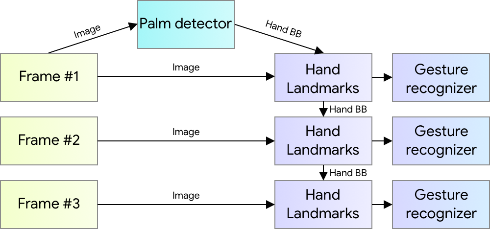
An ML Pipeline for Hand Tracking and Gesture Recognition
Our hand tracking solution utilizes an ML pipeline consisting of several models working together:
  • A palm detector model (called BlazePalm) that operates on the full image and returns an oriented hand bounding box.
  • A hand landmark model that operates on the cropped image region defined by the palm detector and returns high fidelity 3D hand keypoints.
  • A gesture recognizer that classifies the previously computed keypoint configuration into a discrete set of gestures.
This architecture is similar to that employed by our recently published face mesh ML pipeline and that others have used for pose estimation. Providing the accurately cropped palm image to the hand landmark model drastically reduces the need for data augmentation (e.g. rotations, translation and scale) and instead allows the network to dedicate most of its capacity towards coordinate prediction accuracy.
Hand perception pipeline overview.
BlazePalm: Realtime Hand/Palm Detection
To detect initial hand locations, we employ a single-shot detector model called BlazePalm, optimized for mobile real-time uses in a manner similar to BlazeFace, which is also available in MediaPipe. Detecting hands is a decidedly complex task: our model has to work across a variety of hand sizes with a large scale span (~20x) relative to the image frame and be able to detect occluded and self-occluded hands. Whereas faces have high contrast patterns, e.g., in the eye and mouth region, the lack of such features in hands makes it comparatively difficult to detect them reliably from their visual features alone. Instead, providing additional context, like arm, body, or person features, aids accurate hand localization.

Our solution addresses the above challenges using different strategies. First, we train a palm detector instead of a hand detector, since estimating bounding boxes of rigid objects like palms and fists is significantly simpler than detecting hands with articulated fingers. In addition, as palms are smaller objects, the non-maximum suppression algorithm works well even for two-hand self-occlusion cases, like handshakes. Moreover, palms can be modelled using square bounding boxes (anchors in ML terminology) ignoring other aspect ratios, and therefore reducing the number of anchors by a factor of 3-5. Second, an encoder-decoder feature extractor is used for bigger scene context awareness even for small objects (similar to the RetinaNet approach). Lastly, we minimize the focal loss during training to support a large amount of anchors resulting from the high scale variance.

With the above techniques, we achieve an average precision of 95.7% in palm detection. Using a regular cross entropy loss and no decoder gives a baseline of just 86.22%.

Hand Landmark Model
After the palm detection over the whole image our subsequent hand landmark model performs precise keypoint localization of 21 3D hand-knuckle coordinates inside the detected hand regions via regression, that is direct coordinate prediction. The model learns a consistent internal hand pose representation and is robust even to partially visible hands and self-occlusions.

To obtain ground truth data, we have manually annotated ~30K real-world images with 21 3D coordinates, as shown below (we take Z-value from image depth map, if it exists per corresponding coordinate). To better cover the possible hand poses and provide additional supervision on the nature of hand geometry, we also render a high-quality synthetic hand model over various backgrounds and map it to the corresponding 3D coordinates.
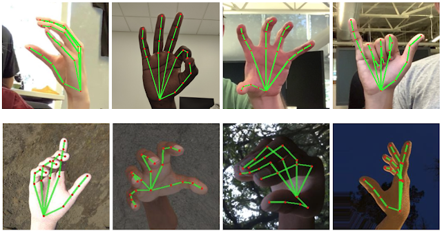
Top: Aligned hand crops passed to the tracking network with ground truth annotation. Bottom: Rendered synthetic hand images with ground truth annotation
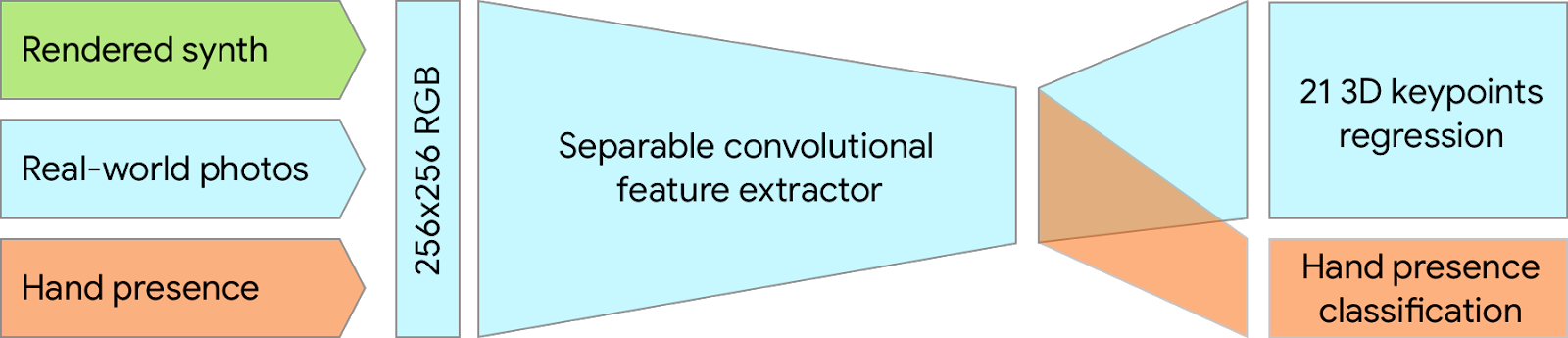
However, purely synthetic data poorly generalizes to the in-the-wild domain. To overcome this problem, we utilize a mixed training schema. A high-level model training diagram is presented in the following figure.
Mixed training schema for hand tracking network. Cropped real-world photos and rendered synthetic images are used as input to predict 21 3D keypoints.
The table below summarizes regression accuracy depending on the nature of the training data. Using both synthetic and real world data results in a significant performance boost.

Mean regression error
Dataset normalized by palm size
Only real-world 16.1 %
Only rendered synthetic 25.7 %
Mixed real-world + synthetic 13.4 %

Gesture Recognition
On top of the predicted hand skeleton, we apply a simple algorithm to derive the gestures. First, the state of each finger, e.g. bent or straight, is determined by the accumulated angles of joints. Then we map the set of finger states to a set of pre-defined gestures. This straightforward yet effective technique allows us to estimate basic static gestures with reasonable quality. The existing pipeline supports counting gestures from multiple cultures, e.g. American, European, and Chinese, and various hand signs including “Thumb up”, closed fist, “OK”, “Rock”, and “Spiderman”.

Implementation via MediaPipe
With MediaPipe, this perception pipeline can be built as a directed graph of modular components, called Calculators. Mediapipe comes with an extendable set of Calculators to solve tasks like model inference, media processing algorithms, and data transformations across a wide variety of devices and platforms. Individual calculators like cropping, rendering and neural network computations can be performed exclusively on the GPU. For example, we employ TFLite GPU inference on most modern phones.

Our MediaPipe graph for hand tracking is shown below. The graph consists of two subgraphs—one for hand detection and one for hand keypoints (i.e., landmark) computation. One key optimization MediaPipe provides is that the palm detector is only run as necessary (fairly infrequently), saving significant computation time. We achieve this by inferring the hand location in the subsequent video frames from the computed hand key points in the current frame, eliminating the need to run the palm detector over each frame. For robustness, the hand tracker model outputs an additional scalar capturing the confidence that a hand is present and reasonably aligned in the input crop. Only when the confidence falls below a certain threshold is the hand detection model reapplied to the whole frame.
The hand landmark model’s output (REJECT_HAND_FLAG) controls when the hand detection model is triggered. This behavior is achieved by MediaPipe’s powerful synchronization building blocks, resulting in high performance and optimal throughput of the ML pipeline.
A highly efficient ML solution that runs in real-time and across a variety of different platforms and form factors involves significantly more complexities than what the above simplified description captures. To this end, we are open sourcing the above hand tracking and gesture recognition pipeline in the MediaPipe framework, accompanied with the relevant end-to-end usage scenario and source code, here. This provides researchers and developers with a complete stack for experimentation and prototyping of novel ideas based on our model.

Future Directions
We plan to extend this technology with more robust and stable tracking, enlarge the amount of gestures we can reliably detect, and support dynamic gestures unfolding in time. We believe that publishing this technology can give an impulse to new creative ideas and applications by the members of the research and developer community at large. We are excited to see what you can build with it!
Acknowledgements
Special thanks to all our team members who worked on the tech with us: Andrey Vakunov, Andrei Tkachenka, Yury Kartynnik, Artsiom Ablavatski, Ivan Grishchenko, Kanstantsin Sokal‎, Mogan Shieh, Ming Guang Yong, Anastasia Tkach, Jonathan Taylor, Sean Fanello, Sofien Bouaziz, Juhyun Lee‎, Chris McClanahan, Jiuqiang Tang‎, Esha Uboweja‎, Hadon Nash‎, Camillo Lugaresi, Michael Hays, Chuo-Ling Chang, Matsvei Zhdanovich and Matthias Grundmann.

Source: Google AI Blog


Video Understanding Using Temporal Cycle-Consistency Learning


In the last few years there has been great progress in the field of video understanding. For example, supervised learning and powerful deep learning models can be used to classify a number of possible actions in videos, summarizing the entire clip with a single label. However, there exist many scenarios in which we need more than just one label for the entire clip. For example, if a robot is pouring water into a cup, simply recognizing the action of “pouring a liquid” is insufficient to predict when the water will overflow. For that, it is necessary to track frame-by-frame the amount of water in the cup as it is being filled. Similarly, a baseball coach who is comparing stances of pitchers may want to retrieve video frames from the precise moment that the ball leaves the pitchers’ hands. Such applications require models to understand each frame of a video.

However, applying supervised learning to understand each individual frame in a video is expensive, since per-frame labels in videos of the action of interest are needed. This requires that annotators apply fine-grained labels to videos by manually adding unambiguous labels to every frame in each video. Only then can the model be trained, and only on a single action. Training on new actions requires the process to be repeated. With the increasing demand for fine-grained labeling, necessary for applications ranging from robotics to sports analytics, this makes the need for scalable learning algorithms that can understand videos without the tedious labeling process increasingly pertinent.

We propose a potential solution using a self-supervised learning method called Temporal Cycle-Consistency Learning (TCC). This novel approach uses correspondences between examples of similar sequential processes to learn representations particularly well-suited for fine-grained temporal understanding of videos. We are also releasing our TCC codebase to enable end-users to apply our self-supervised learning algorithm to new and novel applications.

Representation Learning Using TCC
A plant growing from a seedling to a tree; the daily routine of getting up, going to work and coming back home; or a person pouring themselves a glass of water are all examples of events that happen in a particular order. Videos capturing such processes provide temporal correspondences across multiple instances of the same process. For example, when pouring a drink one could be reaching for a teapot, a bottle of wine, or a glass of water to pour from. Key moments are common to all pouring videos (e.g., the first touch to the container or the container being lifted from the ground) and exist independent of many varying factors, such as visual changes in viewpoint, scale, container style, or the speed of the event. TCC attempts to find such correspondences across videos of the same action by leveraging the principle of cycle-consistency, which has been applied successfully in many problems in computer vision, to learn useful visual representations by aligning videos.

The objective of this training algorithm is to learn a frame encoder, using any network architecture that processes images, such as ResNet. To do so, we pass all frames of the videos to be aligned through the encoder to produce their corresponding embeddings. We then select two videos for TCC learning, say video 1 (the reference video) and video 2. A reference frame is chosen from video 1 and its nearest neighbor frame (NN2) from video 2 is found in the embedding space (not pixel space). We then cycle back by finding the nearest neighbor of NN2 in video 1, which we call NN1. If the representations are cycle-consistent, then the nearest neighbor frame in video 1 (NN1) should refer back to the starting reference frame.
We train the embedder using the distance between the starting reference frame and NN1 as the training signal. As training proceeds, the embeddings improve and reduce the cycle-consistency loss by developing a semantic understanding of each video frame in the context of the action being performed.
Using TCC, we learn embeddings with temporally fine-grained understanding of an action by aligning related videos.
What Does TCC Learn?
In the following figure, we show a model trained using TCC on videos from the Penn Action Dataset of people performing squat exercises. Each point on the left corresponds to frame embeddings, with the highlighted points tracking the embedding of the current video frame. Notice how the embeddings move collectively in spite of many differences in pose, lighting, body and object type. TCC embeddings encode the different phases of squatting without being provided explicit labels.
Right: Input videos of people performing a squat exercise. The video on the top left is the reference. The other videos show nearest neighbor frames (in the TCC embedding space) from other videos of people doing squats. Left: The corresponding frame embeddings move as the action is performed.
Applications of TCC
The learned per-frame embeddings enable an array of interesting applications:
  • Few-shot action phase classification
    When few labeled videos are available for training, the few-shot scenario, TCC performs very well. In fact, TCC can classify the phases of different actions with as few as a single labeled video. In the next figure we compare to other supervised and self-supervised learning approaches in the few-shot setting. We find that supervised learning requires about 50 videos with each frame labeled to achieve the same accuracy that self-supervised methods achieve with just one fully labeled video.
    Comparison of self-supervised and supervised learning for few-shot action phase classification.
  • Unsupervised video alignment
    Aligning or synchronizing videos manually becomes prohibitively difficult as the number of videos increases. Using TCC, many videos can be aligned by selecting the nearest neighbor to each frame in a reference video, without the need for additional labels, as demonstrated in the figure below.
    Results of unsupervised video alignment on videos of people pitching baseball using the distance between frames in the TCC space. The reference video used for alignment is shown in the upper left panel.
  • Label/modality transfer between videos
    Just as TCC finds similar frames by using a nearest neighbor search in the embedding space, it can transfer metadata associated with any frame in one video to its matching frame in another video. This metadata can be in the form of temporal semantic labels or other modalities, such as sound or text. In the video below we show two examples where we can transfer the sound of liquid being poured into a cup from one video to another.
  • Per-frame Retrieval
    With TCC, each frame in a video can be used as a query for retrieval of similar frames by looking up the nearest neighbors in the learned embedding space. The embeddings are powerful enough to differentiate between frames that look quite similar, such as frames just before or after the release of a bowling ball.
    We can perform retrieval from videos on a per-frame basis, i.e., any frame can be used to look up similar frames in a large collection of videos. The retrieved nearest neighbors show that the model captures fine-grained differences in the scene.
Release
We are releasing our codebase, which includes implementations of a number of state-of-the-art self-supervised learning methods, including TCC. This codebase will be useful for researchers working on video understanding, as well as artists looking to use machine learning to align videos to create mosaics of people, animals, and objects moving synchronously.

Acknowledgements
This is joint work with Yusuf Aytar, Jonathan Tompson, Pierre Sermanet, and Andrew Zisserman. The authors would like to thank Alexandre Passos, Allen Lavoie, Anelia Angelova, Bryan Seybold, Priya Gupta, Relja Arandjelović, Sergio Guadarrama, Sourish Chaudhuri, and Vincent Vanhoucke for their help with this project. The videos used in this project come from the PennAction dataset. We thank the creators of PennAction for curating such an interesting dataset.

Source: Google AI Blog


An Interactive, Automated 3D Reconstruction of a Fly Brain


The goal of connectomics research is to map the brain’s "wiring diagram" in order to understand how the nervous system works. A primary target of recent work is the brain of the fruit fly (Drosophila melanogaster), which is a well-established research animal in biology. Eight Nobel Prizes have been awarded for fruit fly research that has led to advances in molecular biology, genetics, and neuroscience. An important advantage of flies is their size: Drosophila brains are relatively small (one hundred thousand neurons) compared to, for example, a mouse brain (one hundred million neurons) or a human brain (one hundred billion neurons). This makes fly brains easier to study as a complete circuit.

Today, in collaboration with the Howard Hughes Medical Institute (HHMI) Janelia Research Campus and Cambridge University, we are excited to publish “Automated Reconstruction of a Serial-Section EM Drosophila Brain with Flood-Filling Networks and Local Realignment”, a new research paper that presents the automated reconstruction of an entire fruit fly brain. We are also making the full results available for anyone to download or to browse online using an interactive, 3D interface we developed called Neuroglancer.
A 40-trillion pixel fly brain reconstruction, open to anyone for interactive viewing. Bottom right: smaller datasets that Google AI analyzed in publications in 2016 and 2018.
Automated Reconstruction of 40 Trillion Pixels
Our collaborators at HHMI sectioned a fly brain into thousands of ultra-thin 40-nanometer slices, imaged each slice using a transmission electron microscope (resulting in over forty trillion pixels of brain imagery), and then aligned the 2D images into a coherent, 3D image volume of the entire fly brain. Using thousands of Cloud TPUs we then applied Flood-Filling Networks (FFNs), which automatically traced each individual neuron in the fly brain.

While the algorithm generally performed well, we found performance degraded when the alignment was imperfect (image content in consecutive sections was not stable) or when occasionally there were multiple consecutive slices missing due to difficulties associated with the sectioning and imaging process. In order to compensate for these issues we combined FFNs with two new procedures. First, we estimated the slice-to-slice consistency everywhere in the 3D image and then locally stabilized the image content as the FFN traced each neuron. Second, we used a “Segmentation-Enhanced CycleGAN” (SECGAN) to computationally “hallucinate” missing slices in the image volume. SECGANs are a type of generative adversarial network specialized for image segmentation. We found that the FFN was able to trace through locations with multiple missing slices much more robustly when using the SECGAN-hallucinated image data.
Interactive Visualization of the Fly Brain with Neuroglancer
When working with 3D images that contain trillions of pixels and objects with complicated shapes, visualization is both essential and difficult. Inspired by Google’s history of developing new visualization technologies, we designed a new tool that was scalable and powerful, but also accessible to anybody with a web browser that supports WebGL. The result is Neuroglancer, an open-source project (github) that enables viewing of petabyte-scale 3D volumes, and supports many advanced features such as arbitrary-axis cross-sectional reslicing, multi-resolution meshes, and the powerful ability to develop custom analysis workflows via integration with Python. This tool has become heavily used by collaborators at the Allen Institute for Brain Science, Harvard University, HHMI, Max Planck Institute, MIT, Princeton University, and elsewhere.
A recorded demonstration of Neuroglancer. Interactive version available here.
Next Steps
Our collaborators at HHMI and Cambridge University have already begun using this reconstruction to accelerate their studies of learning, memory, and perception in the fly brain. However, the results described above are not yet a true connectome since establishing a connectome requires the identification of synapses. We are working closely with the FlyEM team at Janelia Research Campus to create a highly verified and exhaustive connectome of the fly brain using images acquired with “FIB-SEM” technology.

Acknowledgements
We would like to acknowledge core contributions from Tim Blakely, Viren Jain, Michal Januszewski, Laramie Leavitt, Larry Lindsey, Mike Tyka (Google), as well as Alex Bates, Davi Bock, Greg Jefferis, Feng Li, Mathew Nichols, Eric Perlman, Istvan Taisz, and Zhihao Zheng (Cambridge University, HHMI Janelia, Johns Hopkins University, and University of Vermont).

Source: Google AI Blog


Advancing Semi-supervised Learning with Unsupervised Data Augmentation


Success in deep learning has largely been enabled by key factors such as algorithmic advancements, parallel processing hardware (GPU / TPU), and the availability of large-scale labeled datasets, like ImageNet. However, when labeled data is scarce, it can be difficult to train neural networks to perform well. In this case, one can apply data augmentation methods, e.g., paraphrasing a sentence or rotating an image, to effectively increase the amount of labeled training data. Recently, there has been significant progress in the design of data augmentation approaches for a variety of areas such as natural language processing (NLP), vision, and speech. Unfortunately, data augmentation is often limited to supervised learning only, in which labels are required to transfer from original examples to augmented ones.
Example augmentation operations for text-based (top) or image-based (bottom) training data.
In our recent work, “Unsupervised Data Augmentation (UDA) for Consistency Training”, we demonstrate that one can also perform data augmentation on unlabeled data to significantly improve semi-supervised learning (SSL). Our results support the recent revival of semi-supervised learning, showing that: (1) SSL can match and even outperform purely supervised learning that uses orders of magnitude more labeled data, (2) SSL works well across domains in both text and vision and (3) SSL combines well with transfer learning, e.g., when fine-tuning from BERT. We have also open-sourced our code (github) for the community to replicate and build upon.

Unsupervised Data Augmentation Explained
Unsupervised Data Augmentation (UDA) makes use of both labeled data and unlabeled data. To use labeled data, it computes the loss function using standard methods for supervised learning to train the model, as shown in the left part of the graph below. For unlabeled data, consistency training is applied to enforce the predictions to be similar for an unlabeled example and the augmented unlabeled example, as shown in the right part of the graph. Here, the same model is applied to both the unlabeled example and its augmented counterpart to produce two model predictions, from which a consistency loss is computed (i.e., the distance between the two prediction distributions). UDA then computes the final loss by jointly optimizing both the supervised loss from the labeled data and the unsupervised consistency loss from the unlabeled data.

An overview of Unsupervised Data Augmentation (UDA). Left: Standard supervised loss is computed when labeled data is available. Right: With unlabeled data, a consistency loss is computed between an example and its augmented version.
By minimizing the consistency loss, UDA allows for label information to propagate smoothly from labeled examples to unlabeled ones. Intuitively, one can think of UDA as an implicit iterative process. First, the model relies on a small amount of labeled examples to make correct predictions for some unlabeled examples, from which the label information is propagated to augmented counterparts through the consistency loss. Over time, more and more unlabeled examples will be predicted correctly which reflects the improved generalization of the model. Various other types of noise have been tested for consistency training (e.g., Gaussian noise, adversarial noise, and others), yet we found that data augmentation outperforms all of them, leading to state-of-the-art performance on a wide variety of tasks from language to vision. UDA applies different existing augmentation methods depending on the task at hand, including back translation, AutoAugment, and TF-IDF word replacement.

Benchmarks in NLP and Computer Vision
UDA is surprisingly effective in the low-data regime. With only 20 labeled examples, UDA achieves an error rate of 4.20 on the IMDb sentiment analysis task by leveraging 50,000 unlabeled examples. This result outperforms the previous state-of-the-art model trained on 25,000 labeled examples with an error rate of 4.32. In the large-data regime, with the full training set, UDA also provides robust gains.
Benchmark on IMDb, a sentiment analysis task. UDA surpasses state-of-the-art results in supervised learning across different training sizes.
On the CIFAR-10 semi-supervised learning benchmark, UDA outperforms all existing SSL methods, such as VAT, ICT, and MixMatch by significant margins. With 4k examples, UDA achieves an error rate of 5.27, matching the performance of the fully supervised model that uses 50k examples. Furthermore, with a more advanced architecture, PyramidNet+ShakeDrop, UDA achieves a new state-of-the-art error rate of 2.7, a more than 45% reduction in error rate compared to the previous best semi-supervised result. On SVHN, UDA achieves an error rate of 2.85 with only 250 labeled examples, matching the performance of the fully supervised model trained with ~70k labeled examples.
SSL benchmark on CIFAR-10, an image classification task. UDA surpases all existing semi-supervised learning methods, all of which use the Wide-ResNet-28-2 architecture. At 4000 examples, UDA matches the performance of the fully supervised setting with 50,000 examples.
On ImageNet with 10% labeled examples, UDA improves the top-1 accuracy from 55.1% to 68.7%. In the high-data regime with the fully labeled set and 1.3M extra unlabeled examples, UDA continues to provide gains from 78.3% to 79.0% for top-1 accuracy.

Release
We have released the codebase of UDA, together with all data augmentation methods, e.g., back-translation with pre-trained translation models, to replicate our results. We hope that this release will further advance the progress in semi-supervised learning.

Acknowledgements
Special thanks to the co-authors of the paper Zihang Dai, Eduard Hovy, and Quoc V. Le. We’d also like to thank Hieu Pham, Adams Wei Yu, Zhilin Yang, Colin Raffel, Olga Wichrowska, Ekin Dogus Cubuk, Guokun Lai, Jiateng Xie, Yulun Du, Trieu Trinh, Ran Zhao, Ola Spyra, Brandon Yang, Daiyi Peng, Andrew Dai, Samy Bengio and Jeff Dean for their help with this project. A preprint is available online.

Source: Google AI Blog


Announcing the YouTube-8M Segments Dataset


Over the last two years, the First and Second YouTube-8M Large-Scale Video Understanding Challenge and Workshop have collectively drawn 1000+ teams from 60+ countries to further advance large-scale video understanding research. While these events have enabled great progress in video classification, the YouTube dataset on which they were based only used machine-generated video-level labels, and lacked fine-grained temporally localized information, which limited the ability of machine learning models to predict video content.

To accelerate the research of temporal concept localization, we are excited to announce the release of YouTube-8M Segments, a new extension of the YouTube-8M dataset that includes human-verified labels at the 5-second segment level on a subset of YouTube-8M videos. With the additional temporal annotations, YouTube-8M is now both a large-scale classification dataset as well as a temporal localization dataset. In addition, we are hosting another Kaggle video understanding challenge focused on temporal localization, as well as an affiliated 3rd Workshop on YouTube-8M Large-Scale Video Understanding at the 2019 International Conference on Computer Vision (ICCV’19).


YouTube-8M Segments
Video segment labels provide a valuable resource for temporal localization not possible with video-level labels, and enable novel applications, such as capturing special video moments. Instead of exhaustively labeling all segments in a video, to create the YouTube-8M Segments extension, we manually labeled 5 segments (on average) per randomly selected video on the YouTube-8M validation dataset, totalling ~237k segments covering 1000 categories.

This dataset, combined with the previous YouTube-8M release containing a very large number of machine generated video-level labels, should allow learning temporal localization models in novel ways. Evaluating such classifiers is of course very challenging if only noisy video-level labels are available. We hope that the newly added human-labeled annotations will help ensure that researchers can more accurately evaluate their algorithms.

The 3rd YouTube-8M Video Understanding Challenge
This year the YouTube-8M Video Understanding Challenge focuses on temporal localization. Participants are encouraged to leverage noisy video-level labels together with a small segment-level validation set in order to better annotate and temporally localize concepts of interest. Unlike last year, there is no model size restriction. Each of the top 10 teams will be awarded $2,500 to support their travel to Seoul to attend ICCV’19. For details, please visit the Kaggle competition page.

The 3rd Workshop on YouTube-8M Large-Scale Video Understanding
Continuing in the tradition of the previous two years, the 3rd workshop will feature four invited talks by distinguished researchers as well as presentations by top-performing challenge participants. We encourage those who wish to attend to submit papers describing their research, experiments, or applications based on the YouTube-8M dataset, including papers summarizing their participation in the challenge above. Please refer to the workshop page for more details.

It is our hope that this newest extension will serve as a unique playground for temporal localization that mimics real world scenarios. We also look forward to the new challenge and workshop, which we believe will continue to advance research in large-scale video understanding. We hope you will join us again!

Acknowledgements
This post reflects the work of many machine perception researchers including Ke Chen, Nisarg Kothari, Joonseok Lee, Hanhan Li, Paul Natsev, Joe Yue-Hei Ng, Naderi Parizi, David Ross, Cordelia Schmid, Javier Snaider, Rahul Sukthankar, George Toderici, Balakrishnan Varadarajan, Sudheendra Vijayanarasimhan, Yexin Wang, Zheng Xu, as well as Julia Elliott and Walter Reade from Kaggle. We are also grateful for the support and advice from our partners at YouTube.

Source: Google AI Blog