Tag Archives: Computer Vision

Leveraging Temporal Context for Object Detection


Ecological monitoring helps researchers to understand the dynamics of global ecosystems, quantify biodiversity, and measure the effects of climate change and human activity, including the efficacy of conservation and remediation efforts. In order to monitor effectively, ecologists need high-quality data, often expending significant efforts to place monitoring sensors, such as static cameras, in the field. While it is increasingly cost effective to build and operate networks of such sensors, the manual data analysis of global biodiversity data remains a bottleneck to accurate, global, real-time ecological monitoring. While there are ways to automate this analysis via machine learning, the data from static cameras, widely used to monitor the world around us for purposes ranging from mountain pass road conditions to ecosystem phenology, still pose a strong challenge for traditional computer vision systems — due to power and storage constraints, sampling frequencies are low, often no faster than one frame per second, and sometimes are irregular due to the use of a motion trigger.

In order to perform well in this setting, computer vision models must be robust to objects of interest that are often off-center, out of focus, poorly lit, or at a variety of scales. In addition, a static camera will always take images of the same scene unless it is moved, which causes the data from any one camera to be highly repetitive. Without sufficient data variability, machine learning models may learn to focus on correlations in the background, leading to poor generalization to novel deployments. The machine learning and ecological communities have been working together through venues like LILA BC and Wildlife Insights to curate expert-labeled training data from many research groups, each of which may operate anywhere from one to hundreds of camera traps, in order to increase data variability. This process of data collection and annotation is slow, and is confounded by the need to have diverse, representative data across geographic regions and taxonomic groups.
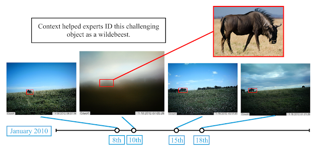
What’s in this image? Objects in images from static cameras can be very challenging to detect and categorize. Here, a foggy morning has made it very difficult to see a herd of wildebeest walking along the crest of a hill. [Image from Snapshot Serengeti]
In Context R-CNN: Long Term Temporal Context for Per-Camera Object Detection, we present a complementary approach that increases global scalability by improving generalization to novel camera deployments algorithmically. This new object detection architecture leverages contextual clues across time for each camera deployment in a network, improving recognition of objects in novel camera deployments without relying on additional training data from a large number of cameras. Echoing the approach a person might use when faced with challenging images, Context R-CNN leverages up to a month’s worth of images from the same camera for context to determine what objects might be present and identify them. Using this method, the model outperforms a single-frame Faster R-CNN baseline by significant margins across multiple domains, including wildlife camera traps. We have open sourced the code and models for this work as part of the TF Object Detection API to make it easy to train and test Context R-CNN models on new static camera datasets.
Here, we can see how additional examples from the same scene help experts determine that the object is an animal and not background. Context such as the shape & size of the object, its attachment to a herd, and habitual grazing at certain times of day help determine that the species is a wildebeest. Useful examples occur throughout the month.
The Context R-CNN Model
Context R-CNN is designed to take advantage of the high degree of correlation within images taken by a static camera to boost performance on challenging data and improve generalization to new camera deployments without additional human data labeling. It is an adaptation of Faster R-CNN, a popular two-stage object detection architecture. To extract context for a camera, we first use a frozen feature extractor to build up a contextual memory bank from images across a large time horizon (up to a month or more). Next, objects are detected in each image using Context R-CNN which aggregates relevant context from the memory bank to help detect objects under challenging conditions (such as the heavy fog obscuring the wildebeests in our previous example). This aggregation is performed using attention, which is robust to the sparse and irregular sampling rates often seen in static monitoring cameras.
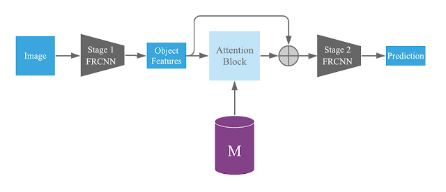
High-level architecture diagram, showing how Context R-CNN incorporates long-term context within the Faster R-CNN model architecture.
The first stage of Faster R-CNN proposes potential objects, and the second stage categorizes each proposal as either background or one of the target classes. In Context R-CNN, we take the proposed objects from the first stage of Faster R-CNN, and for each one we use similarity-based attention to determine how relevant each of the features in our memory bank (M) is to the current object, and construct a per-object context feature by taking a relevance-weighted sum over M and adding it back to the original object features. Then each object, now with added contextual information, is finally categorized using the second stage of Faster R-CNN.
Context R-CNN is able to leverage context (spanning up to 1 month) to correctly categorize the challenging wildebeest example we saw above. The green values are the corresponding attention weights for each boxed object.
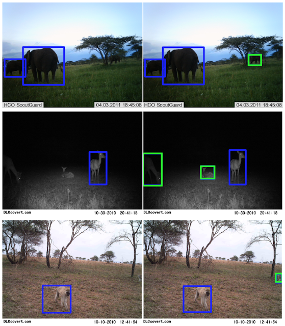
Compared to a Faster R-CNN baseline (left), Context R-CNN (right) is able to capture challenging objects such as an elephant occluded by a tree, two poorly-lit impala, and a vervet monkey leaving the frame. [Images from Snapshot Serengeti]
Results
We have tested Context R-CNN on Snapshot Serengeti (SS) and Caltech Camera Traps (CCT), both ecological datasets of animal species in camera traps but from highly different geographic regions (Tanzania vs. the Southwestern United States). Improvements over the Faster R-CNN baseline for each dataset can be seen in the table below. Notably, we see a 47.5% relative increase in mean average precision (mAP) on SS, and a 34.3% relative mAP increase on CCT. We also compare Context R-CNN to S3D (a 3D convolution based baseline) and see performance improve from 44.7% mAP to 55.9% mAP (a 25.1% relative increase). Finally, we find that the performance increases as the contextual time horizon increases, from a minute of context to a month.
Comparison to a single frame Faster R-CNN baseline, showing both mean average precision (mAP) and average recall (AR) detection metrics.
Ongoing and Future Work
We are working to implement Context R-CNN within the Wildlife Insights platform, to facilitate large-scale, global ecological monitoring via camera traps. We also host competitions such as the yearly iWildCam species identification competition at the CVPR Fine-Grained Visual Recognition Workshop to help bring these challenges to the attention of the computer vision community. The challenges seen in automatic species identification in static cameras are shared by numerous applications of static cameras outside of the ecological monitoring domain, as well as other static sensors used to monitor biodiversity, such as audio and sonar devices. Our method is general, and we anticipate the per-sensor context approach taken by Context R-CNN would be beneficial for any static sensor.

Acknowledgements
This post reflects the work of the authors as well as the following group of core contributors: Vivek Rathod, Guanhang Wu, Ronny Votel. We are also grateful to Zhichao Lu, David Ross, Tanya Birch and the Wildlife Insights AI team, and Pietro Perona and the Caltech Computational Vision Lab.
Source: Google AI Blog


RepNet: Counting Repetitions in Videos


Repeating processes ranging from natural cycles, such as phases of the moon or heartbeats and breathing, to artificial repetitive processes, like those found on manufacturing lines or in traffic patterns, are commonplace in our daily lives. Beyond just their prevalence, repeating processes are of interest to researchers for the variety of insights one can tease out of them. It may be that there is an underlying cause behind something that happens multiple times, or there may be gradual changes in a scene that may be useful for understanding. Sometimes, repeating processes provide us with unambiguous “action units”, semantically meaningful segments that make up an action. For example, if a person is chopping an onion, the action unit is the manipulation action that is repeated to produce additional slices. These units may be indicative of more complex activity and may allow us to analyze more such actions automatically at a finer time-scale without having a person annotate these units. For the above reasons, perceptual systems that aim to observe and understand our world for an extended period of time will benefit from a system that understands general repetitions.

In “Counting Out Time: Class Agnostic Video Repetition Counting in the Wild”, we present RepNet, a single model that can understand a broad range of repeating processes, ranging from people exercising or using tools, to animals running and birds flapping their wings, pendulums swinging, and a wide variety of others. In contrast to our previous work, which used cycle-consistency constraints across different videos of the same action to understand them at a fine-grained level, in this work we present a system that can recognize repetitions within a single video. Along with this model, we are releasing a dataset to benchmark class-agnostic counting in videos and a Colab notebook to run RepNet.

RepNet
RepNet is a model that takes as input a video that contains periodic action of a variety of classes (including those unseen during training) and returns the period of repetitions found therein. In the past the problem of repetition counting has been addressed by directly comparing pixel intensities in frames, but real world videos have camera motion, occlusion by objects in the field, drastic scale difference and changes in form, which necessitates learning of features invariant to such noise. To accomplish this we train a machine learning model in an end-to-end manner to directly estimate the period of the repetitions. The model consists of three parts: a frame encoder, an intermediate representation, called a temporal self-similarity matrix (which we will describe below), and a period predictor.

First, the frame encoder uses the ResNet architecture as a per-frame model to generate embeddings of each frame of the video The ResNet architecture was chosen since it has been successful for a number of image and video tasks. Passing each frame of a video through a ResNet-based encoder yields a sequence of embeddings.

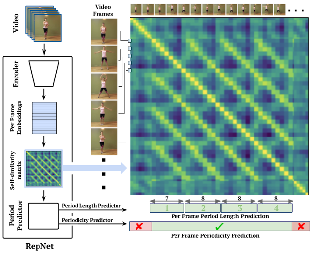
At this point we calculate a temporal self-similarity matrix (TSM) by comparing each frame’s embedding with every other frame in the video, returning a matrix that is easy for subsequent modules to analyze for counting repetitions. This process surfaces self-similarities in the stream of video frames that enable period estimation, as demonstrated in the video below.
Demonstration of how the TSM processes images of the Earth’s day-night cycle.
For each frame, we then use Transformers to predict the period of repetition and the periodicity (i.e., whether or not a frame is part of the periodic process) directly from the sequence of similarities in the TSM. Once we have the period, we obtain the per-frame count by dividing the number of frames captured in a periodic segment by the period length. We sum this up to predict the number of repetitions in the video.
Overview of the RepNet model.
Temporal Self-Similarity Matrix
The example of the TSM from the day-night cycle, shown above, is derived from an idealized scenario with fixed period repetitions. TSMs from real videos often reveal fascinating structures in the world, as demonstrated in the three examples below. Jumping jacks are close to the ideal periodic action with a fixed period, while in contrast, the period of a bouncing ball declines as the ball loses energy through repeated bounces. The video of someone mixing concrete demonstrates repetitive action that is preceded and followed by a period without motion. These three behaviors are clearly distinguished in the learned TSM, which requires that the model pay attention to fine changes in the scene.
Jumping Jacks (constant period; video from Kinetics), Bouncing ball (decreasing period; Kinetics), Mixing concrete (aperiodic segments present in video; PERTUBE dataset).
One advantage of using the TSM as an intermediate layer in RepNet is that the subsequent processing by the transformers is done in the self-similarity space and not in the feature space. This encourages generalization to unseen classes. For example, the TSMs produced by actions as different as jumping jacks or swimming are similar as long as the action was repeated at a similar pace. This allows us to train on some classes and yet expect generalization to unseen classes.

Data
One way to train the above model would be to collect a large dataset of videos that capture repetitive activities and label them with the repetition count. The challenge in this is two-fold. First, it requires one to examine a large number of videos to identify those with repeated actions. Following that, each video must be annotated with the number of times an action was repeated. While for certain tasks annotators can skip frames (for example, to classify a video as showing jumping jacks), they still need to see the entire video in order to count how many jumping jacks were performed.

We overcome this challenge by introducing a process for synthetic data generation that produces videos with repetitions using videos that may not contain repeating actions at all. This is accomplished by randomly selecting a segment of the video to repeat an arbitrary number of times, bookended by the original video context.
Our synthetic data generation pipeline that produces videos with repetitions from any video.
While this process generates a video that resembles a natural-looking video with repeating processes, it is still too simple for deep learning methods, which can learn to cheat by looking for artifacts, instead of learning to recognize repetitions. To address this, we perform extreme data augmentation, which we call camera motion augmentation. In this method, we modify the video to simulate a camera that smoothly moves around using 2D affine motion as the video progresses.
Left: An example of a synthetic repeating video generated from a random video. Right: An example of a video with camera motion augmentation, which is tougher for the model, but results in better generalization to real repeating videos (both from Kinetics).
Evaluation
Even though we can train a model on synthetic repeating videos, the resulting models must be able to generalize to real video of repeating processes. In order to evaluate the performance of the trained models on real videos, we collect a dataset of ~9000 videos from the Kinetics dataset. These videos span many action classes and capture diverse scenes, arising from the diversity of data seen on Youtube. We annotate these videos with the count of the action being repeated in the video. To encourage further research in this field, we are releasing the count annotations for this dataset, which we call Countix.

Applications
A class-agnostic counting model has many useful applications. RepNet serves as a single model that can count repetitions from many different domains:
RepNet can count repeated activities from a range of domains, such as slicing onions (left; video from Kinetics dataset), Earth’s diurnal cycle (middle; Himawari satellite data), or even a cheetah in motion (right; video from imgur.com).
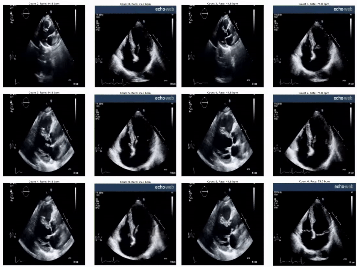
RepNet could be used to estimate heartbeat rates from echocardiogram videos even though it has not seen such videos in training:
Predicted heart rates: 45 bpm (left) and 75 bpm (right). True heart rates 46-50 bpm and 78-79 bpm, respectively. RepNet’s prediction of the heart rate across different devices is encouragingly close to the rate measured by the device. (Source for left and right)
RepNet can also be used to monitor repeating activities for any changes in speed. Below we show how the Such changes in speed can also be used in other settings for quality or process control.
In this video, we see RepNet counting accelerating cellular oscillations observed under a laser microscope even though it has never seen such a video during training, (from Nature article).
Left: Person performing a “mountain climber” exercise. Right: The 1D projection of the RepNet embeddings using principal component analysis, capturing the moment that the person changes their speed during the exercise. (Video from Kinetics)
Release
We are releasing Countix annotations for the community to work on the problem of repetition counting. We are also releasing a Colab notebook for running RepNet. Using this you can run RepNet on your videos or even using your webcam to detect periodic activities in video and count repetitions automatically in videos.

Acknowledgements
This is joint work with Yusuf Aytar, Jonathan Tompson, Pierre Sermanet, and Andrew Zisserman. Special thanks to Tom Small for designing the visual explanation of TSM. The authors thank Anelia Angelova, Relja Arandjelović, Sourish Chaudhuri, Aishwarya Gomatam, Meghana Thotakuri, and Vincent Vanhoucke for their help with this project.

Source: Google AI Blog


Google at CVPR 2020


This week marks the start of the fully virtual 2020 Conference on Computer Vision and Pattern Recognition (CVPR 2020), the premier annual computer vision event consisting of the main conference, workshops and tutorials. As a leader in computer vision research and a Supporter Level Virtual Sponsor, Google will have a strong presence at CVPR 2020, with nearly 70 publications accepted, along with the organization of, and participation in, multiple workshops/tutorials.

If you are participating in CVPR this year, please visit our virtual booth to learn about what Google is actively pursuing for the next generation of intelligent systems that utilize the latest machine learning techniques applied to various areas of machine perception.

You can also learn more about our research being presented at CVPR 2020 in the list below (Google affiliations are bolded).

Organizing Committee

General Chairs: Terry Boult, Gerard Medioni, Ramin Zabih
Program Chairs: Ce Liu, Greg Mori, Kate Saenko, Silvio Savarese
Workshop Chairs: Tal Hassner, Tali Dekel
Website Chairs: Tianfan Xue, Tian Lan
Technical Chair: Daniel Vlasic
Area Chairs include: Alexander Toshev, Alexey Dosovitskiy, Boqing Gong, Caroline Pantofaru, Chen Sun, Deqing Sun, Dilip Krishnan, Feng Yang, Liang-Chieh Chen, Michael Rubinstein, Rodrigo Benenson, Timnit Gebru, Thomas Funkhouser, Varun Jampani, Vittorio Ferrari, William Freeman

Oral Presentations

Evolving Losses for Unsupervised Video Representation Learning
AJ Piergiovanni, Anelia Angelova, Michael Ryoo

CvxNet: Learnable Convex Decomposition
Boyang Deng, Kyle Genova, Soroosh Yazdani, Sofien Bouaziz, Geoffrey Hinton, Andrea Tagliasacchi

Neural SDE: Stabilizing Neural ODE Networks with Stochastic Noise
Xuanqing Liu, Tesi Xiao, Si Si, Qin Cao, Sanjiv Kumar, Cho-Jui Hsieh

Scalability in Perception for Autonomous Driving: Waymo Open Dataset
Pei Sun, Henrik Kretzschmar, Xerxes Dotiwalla‎, Aurélien Chouard, Vijaysai Patnaik, Paul Tsui, James Guo, Yin Zhou, Yuning Chai, Benjamin Caine, Vijay Vasudevan, Wei Han, Jiquan Ngiam, Hang Zhao, Aleksei Timofeev‎, Scott Ettinger, Maxim Krivokon, Amy Gao, Aditya Joshi‎, Sheng Zhao, Shuyang Chen, Yu Zhang, Jon Shlens, Zhifeng Chen, Dragomir Anguelov

Deep Implicit Volume Compression
Saurabh Singh, Danhang Tang, Cem Keskin, Philip Chou, Christian Haene, Mingsong Dou, Sean Fanello, Jonathan Taylor, Andrea Tagliasacchi, Philip Davidson, Yinda Zhang, Onur Guleryuz, Shahram Izadi, Sofien Bouaziz

Neural Networks Are More Productive Teachers Than Human Raters: Active Mixup for Data-Efficient Knowledge Distillation from a Blackbox Model
Dongdong Wan, Yandong Li, Liqiang Wang, and Boqing Gong

Google Landmarks Dataset v2 - A Large-Scale Benchmark for Instance-Level Recognition and Retrieval (see the blog post)
Tobias Weyand, Andre Araujo, Jack Sim, Bingyi Cao

CycleISP: Real Image Restoration via Improved Data Synthesis
Syed Waqas Zamir, Aditya Arora, Salman Khan, Munawar Hayat, Fahad Shahbaz Khan, Ming-Hsuan Yang, Ling Shao

Dynamic Graph Message Passing Networks
Li Zhang, Dan Xu, Anurag Arnab, Philip Torr

Local Deep Implicit Functions for 3D Shape
Kyle Genova, Forrester Cole, Avneesh Sud, Aaron Sarna, Thomas Funkhouser

GHUM & GHUML: Generative 3D Human Shape and Articulated Pose Models
Hongyi Xu, Eduard Gabriel Bazavan, Andrei Zanfir, William Freeman, Rahul Sukthankar, Cristian Sminchisescu

Search to Distill: Pearls are Everywhere but not the Eyes
Yu Liu, Xuhui Jia, Mingxing Tan, Raviteja Vemulapalli, Yukun Zhu, Bradley Green, Xiaogang Wang

Semantic Pyramid for Image Generation
Assaf Shocher, Yossi Gandelsman, Inbar Mosseri, Michal Yarom, Michal Irani, William Freeman, Tali Dekel

Flow Contrastive Estimation of Energy-Based Models
Ruiqi Gao, Erik Nijkamp, Diederik Kingma, Zhen Xu, Andrew Dai, Ying Nian Wu

Rethinking Class-Balanced Methods for Long-Tailed Visual Recognition from A Domain Adaptation Perspective
Muhammad Abdullah Jamal, Matthew Brown, Ming-Hsuan Yang, Liqiang Wang, Boqing Gong

Category-Level Articulated Object Pose Estimation
Xiaolong Li, He Wang, Li Yi, Leonidas Guibas, Amos Abbott, Shuran Song

AdaCoSeg: Adaptive Shape Co-Segmentation with Group Consistency Loss
Chenyang Zhu, Kai Xu, Siddhartha Chaudhuri, Li Yi, Leonidas Guibas, Hao Zhang

SpeedNet: Learning the Speediness in Videos
Sagie Benaim, Ariel Ephrat, Oran Lang, Inbar Mosseri, William Freeman, Michael Rubinstein, Michal Irani, Tali Dekel

BSP-Net: Generating Compact Meshes via Binary Space Partitioning
Zhiqin Chen, Andrea Tagliasacchi, Hao Zhang

SAPIEN: A SimulAted Part-based Interactive ENvironment
Fanbo Xiang, Yuzhe Qin, Kaichun Mo, Yikuan Xia, Hao Zhu, Fangchen Liu, Minghua Liu, Hanxiao Jiang, Yifu Yuan, He Wang, Li Yi, Angel Chang, Leonidas Guibas, Hao Su

SurfelGAN: Synthesizing Realistic Sensor Data for Autonomous Driving
Zhenpei Yang, Yuning Chai, Dragomir Anguelov, Yin Zhou, Pei Sun, Dumitru Erhan, Sean Rafferty, Henrik Kretzschmar

Filter Response Normalization Layer: Eliminating Batch Dependence in the Training of Deep Neural Networks
Saurabh Singh, Shankar Krishnan

RL-CycleGAN: Reinforcement Learning Aware Simulation-To-Real
Kanishka Rao, Chris Harris, Alex Irpan, Sergey Levine, Julian Ibarz, Mohi Khansari

Open Compound Domain Adaptation
Ziwei Liu, Zhongqi Miao, Xingang Pan, Xiaohang Zhan, Dahua Lin, Stella X.Yu, and Boqing Gong

Posters
Single-view view synthesis with multiplane images
Richard Tucker, Noah Snavely

Adversarial Examples Improve Image Recognition
Cihang Xie, Mingxing Tan, Boqing Gong, Jiang Wang, Alan Yuille, Quoc V. Le

Adversarial Texture Optimization from RGB-D Scans
Jingwei Huang, Justus Thies, Angela Dai, Abhijit Kundu, Chiyu “Max” Jiang,Leonidas Guibas, Matthias Niessner, Thomas Funkhouser

Single-Image HDR Reconstruction by Learning to Reverse the Camera Pipeline
Yu-Lun Liu, Wei-Sheng Lai, Yu-Sheng Chen, Yi-Lung Kao, Ming-Hsuan Yang,Yung-Yu Chuang, Jia-Bin Huang

Collaborative Distillation for Ultra-Resolution Universal Style Transfer
Huan Wang, Yijun Li, Yuehai Wang, Haoji Hu, Ming-Hsuan Yang

Learning to Autofocus
Charles Herrmann, Richard Strong Bowen, Neal Wadhwa, Rahul Garg, Qiurui He, Jonathan T. Barron, Ramin Zabih

Multi-Scale Boosted Dehazing Network with Dense Feature Fusion
Hang Dong, Jinshan Pan, Lei Xiang, Zhe Hu, Xinyi Zhang, Fei Wang, Ming-Hsuan Yang

Composing Good Shots by Exploiting Mutual Relations
Debang Li, Junge Zhang, Kaiqi Huang, Ming-Hsuan Yang

PatchVAE: Learning Local Latent Codes for Recognition
Kamal Gupta, Saurabh Singh, Abhinav Shrivastava

Neural Voxel Renderer: Learning an Accurate and Controllable Rendering Tool
Konstantinos Rematas, Vittorio Ferrari

Local Implicit Grid Representations for 3D Scenes
Chiyu “Max” Jiang, Avneesh Sud, Ameesh Makadia, Jingwei Huang, Matthias Niessner, Thomas Funkhouser

Large Scale Video Representation Learning via Relational Graph Clustering
Hyodong Lee, Joonseok Lee, Joe Yue-Hei Ng, Apostol (Paul) Natsev

Deep Homography Estimation for Dynamic Scenes
Hoang Le, Feng Liu, Shu Zhang, Aseem Agarwala

C-Flow: Conditional Generative Flow Models for Images and 3D Point Clouds
Albert Pumarola, Stefan Popov, Francesc Moreno-Noguer, Vittorio Ferrari

Lighthouse: Predicting Lighting Volumes for Spatially-Coherent Illumination
Pratul Srinivasan, Ben Mildenhall, Matthew Tancik, Jonathan T. Barron, Richard Tucker, Noah Snavely

Scale-space flow for end-to-end optimized video compression
Eirikur Agustsson, David Minnen, Nick Johnston, Johannes Ballé, Sung Jin Hwang, George Toderici

StructEdit: Learning Structural Shape Variations
Kaichun Mo, Paul Guerrero, Li Yi, Hao Su, Peter Wonka, Niloy Mitra, Leonidas Guibas

3D-MPA: Multi Proposal Aggregation for 3D Semantic Instance Segmentation
Francis Engelmann, Martin Bokeloh, Alireza Fathi, Bastian Leibe, Matthias Niessner

Sequential mastery of multiple tasks: Networks naturally learn to learn and forget to forget
Guy Davidson, Michael C. Mozer

Distilling Effective Supervision from Severe Label Noise
Zizhao Zhang, Han Zhang, Sercan Ö. Arik, Honglak Lee, Tomas Pfister

ViewAL: Active Learning With Viewpoint Entropy for Semantic Segmentation
Yawar Siddiqui, Julien Valentin, Matthias Niessner

Attribution in Scale and Space
Shawn Xu, Subhashini Venugopalan, Mukund Sundararajan

Weakly-Supervised Semantic Segmentation via Sub-category Exploration
Yu-Ting Chang, Qiaosong Wang, Wei-Chih Hung, Robinson Piramuthu, Yi-Hsuan Tsai, Ming-Hsuan Yang

Speech2Action: Cross-modal Supervision for Action Recognition
Arsha Nagrani, Chen Sun, David Ross, Rahul Sukthankar, Cordelia Schmid, Andrew Zisserman

Counting Out Time: Class Agnostic Video Repetition Counting in the Wild
Debidatta Dwibedi, Yusuf Aytar, Jonathan Tompson, Pierre Sermanet, Andrew Zisserman

The Garden of Forking Paths: Towards Multi-Future Trajectory Prediction
Junwei Liang, Lu Jiang, Kevin Murphy, Ting Yu, Alexander Hauptmann

Self-training with Noisy Student improves ImageNet classification
Qizhe Xie, Minh-Thang Luong, Eduard Hovy, Quoc V. Le

EfficientDet: Scalable and Efficient Object Detection (see the blog post)
Mingxing Tan, Ruoming Pang, Quoc Le

ACNe: Attentive Context Normalization for Robust Permutation-Equivariant Learning
Weiwei Sun, Wei Jiang, Eduard Trulls, Andrea Tagliasacchi, Kwang Moo Yi

VectorNet: Encoding HD Maps and Agent Dynamics from Vectorized Representation
Jiyang Gao, Chen Sun, Hang Zhao, Yi Shen, Dragomir Anguelov, Cordelia Schmid, Congcong Li

SpineNet: Learning Scale-Permuted Backbone for Recognition and Localization
Xianzhi Du, Tsung-Yi Lin, Pengchong Jin, Golnaz Ghiasi, Mingxing Tan, Yin Cui, Quoc Le, Xiaodan Song

KeyPose: Multi-View 3D Labeling and Keypoint Estimation for Transparent Objects
Xingyu Liu, Rico Jonschkowski, Anelia Angelova, Kurt Konolige

Structured Multi-Hashing for Model Compression
Elad Eban, Yair Movshovitz-Attias, Hao Wu, Mark Sandler, Andrew Poon, Yerlan Idelbayev, Miguel A. Carreira-Perpinan

DOPS: Learning to Detect 3D Objects and Predict their 3D Shapes
Mahyar Najibi, Guangda Lai, Abhijit Kundu, Zhichao Lu, Vivek Rathod, Tom Funkhouser, Caroline Pantofaru, David Ross, Larry Davis, Alireza Fathi

Panoptic-DeepLab: A Simple, Strong, and Fast Baseline for Bottom-Up Panoptic Segmentation
Bowen Cheng, Maxwell Collins, Yukun Zhu, Ting Liu, Thomas S. Huang, Hartwig Adam, Liang-Chieh Chen

Context R-CNN: Long Term Temporal Context for Per-Camera Object Detection
Sara Beery, Guanhang Wu, Vivek Rathod, Ronny Votel, Jonathan Huang

Distortion Agnostic Deep Watermarking
Xiyang Luo, Ruohan Zhan, Huiwen Chang, Feng Yang, Peyman Milanfar

Can weight sharing outperform random architecture search? An investigation with TuNAS
Gabriel Bender, Hanxiao Liu, Bo Chen, Grace Chu, Shuyang Cheng, Pieter-Jan Kindermans, Quoc Le

GIFnets: Differentiable GIF Encoding Framework
Innfarn Yoo, Xiyang Luo, Yilin Wang, Feng Yang, Peyman Milanfar

Your Local GAN: Designing Two Dimensional Local Attention Mechanisms for Generative Models
Giannis Daras, Augustus Odena, Han Zhang, Alex Dimakis

Fast Sparse ConvNets
Erich Elsen, Marat Dukhan, Trevor Gale, Karen Simonyan

RetinaTrack: Online Single Stage Joint Detection and Tracking
Zhichao Lu, Vivek Rathod, Ronny Votel, Jonathan Huang

Learning to See Through Obstructions
Yu-Lun Liu, Wei-Sheng Lai, Ming-Hsuan Yang,Yung-Yu Chuang, Jia-Bin Huang

Self-Supervised Learning of Video-Induced Visual Invariances
Michael Tschannen, Josip Djolonga, Marvin Ritter, Aravindh Mahendran, Neil Houlsby, Sylvain Gelly, Mario Lucic

Workshops

3rd Workshop and Challenge on Learned Image Compression
Organizers include: George Toderici, Eirikur Agustsson, Lucas Theis, Johannes Ballé, Nick Johnston

CLVISION 1st Workshop on Continual Learning in Computer Vision
Organizers include: Zhiyuan (Brett) Chen, Marc Pickett

Embodied AI
Organizers include: Alexander Toshev, Jie Tan, Aleksandra Faust, Anelia Angelova

The 1st International Workshop and Prize Challenge on Agriculture-Vision: Challenges & Opportunities for Computer Vision in Agriculture
Organizers include: Zhen Li, Jim Yuan

Embodied AI
Organizers include: Alexander Toshev, Jie Tan, Aleksandra Faust, Anelia Angelova

New Trends in Image Restoration and Enhancement workshop and challenges on image and video restoration and enhancement (NTIRE)
Talk: “Sky Optimization: Semantically aware image processing of skies in low-light photography”
Orly Liba, Longqi Cai, Yun-Ta Tsai, Elad Eban, Yair Movshovitz-Attias, Yael Pritch, Huizhong Chen, Jonathan Barron

The End-of-End-to-End A Video Understanding Pentathlon
Organizers include: Rahul Sukthankar

4th Workshop on Media Forensics
Organizers include: Christoph Bregler

4th Workshop on Visual Understanding by Learning from Web Data
Organizers include: Jesse Berent, Rahul Sukthankar

AI for Content Creation
Organizers include: Deqing Sun, Lu Jiang, Weilong Yang

Fourth Workshop on Computer Vision for AR/VR
Organizers include: Sofien Bouaziz

Low-Power Computer Vision Competition (LPCVC)
Organizers include: Bo Chen, Andrew Howard, Jaeyoun Kim

Sight and Sound
Organizers include: William Freeman

Workshop on Efficient Deep Learning for Computer Vision
Organizers include: Pete Warden

Extreme classification in computer vision
Organizers include: Ramin Zabih, Zhen Li

Image Matching: Local Features and Beyond (see the blog post)
Organizers include: Eduard Trulls

The DAVIS Challenge on Video Object Segmentation
Organizers include: Alberto Montes, Jordi Pont-Tuset, Kevis-Kokitsi Maninis

2nd Workshop on Precognition: Seeing through the Future
Organizers include: Utsav Prabhu

Computational Cameras and Displays (CCD)
Talk: Orly Liba

2nd Workshop on Learning from Unlabeled Videos (LUV)
Organizers include:Honglak Lee, Rahul Sukthankar

7th Workshop on Fine Grained Visual Categorization (FGVC7) (see the blog post)
Organizers include: Christine Kaeser-Chen, Serge Belongie

Language & Vision with applications to Video Understanding
Organizers include: Lu Jiang

Neural Architecture Search and Beyond for Representation Learning
Organizers include: Barret Zoph

Tutorials

Disentangled 3D Representations for Relightable Performance Capture of Humans
Organizers include: Sean Fanello, Christoph Rhemann, Jonathan Taylor, Sofien Bouaziz, Adarsh Kowdle, Rohit Pandey, Sergio Orts-Escolano, Paul Debevec, Shahram Izadi

Learning Representations via Graph-Structured Networks
Organizers include:Chen Sun, Ming-Hsuan Yang

Novel View Synthesis: From Depth-Based Warping to Multi-Plane Images and Beyond
Organizers include:Varun Jampani

How to Write a Good Review
Talks by:Vittorio Ferrari, Bill Freeman, Jordi Pont-Tuset

Neural Rendering
Organizers include:Ricardo Martin-Brualla, Rohit K. Pandey, Sean Fanello,Maneesh Agrawala, Dan B. Goldman

Fairness Accountability Transparency and Ethics and Computer Vision
Organizers: Timnit Gebru, Emily Denton

Source: Google AI Blog


Open-Sourcing BiT: Exploring Large-Scale Pre-training for Computer Vision


A common refrain for computer vision researchers is that modern deep neural networks are always hungry for more labeled data — current state-of-the-art CNNs need to be trained on datasets such as OpenImages or Places, which consist of over 1M labelled images. However, for many applications, collecting this amount of labeled data can be prohibitive to the average practitioner.

A common approach to mitigate the lack of labeled data for computer vision tasks is to use models that have been pre-trained on generic data (e.g., ImageNet). The idea is that visual features learned on the generic data can be re-used for the task of interest. Even though this pre-training works reasonably well in practice, it still falls short of the ability to both quickly grasp new concepts and understand them in different contexts. In a similar spirit to how BERT and T5 have shown advances in the language domain, we believe that large-scale pre-training can advance the performance of computer vision models.

In “Big Transfer (BiT): General Visual Representation Learning” we devise an approach for effective pre-training of general features using image datasets at a scale beyond the de-facto standard (ILSVRC-2012). In particular, we highlight the importance of appropriately choosing normalization layers and scaling the architecture capacity as the amount of pre-training data increases. Our approach exhibits unprecedented performance adapting to a wide range of new visual tasks, including the few-shot recognition setting and the recently introduced “real-world” ObjectNet benchmark. We are excited to share the best BiT models pre-trained on public datasets, along with code in TF2, Jax, and PyTorch. This will allow anyone to reach state-of-the-art performance on their task of interest, even with just a handful of labeled images per class.

Pre-training
In order to investigate the effect of data scale, we revisit common design choices of the pre-training setup (such as normalizations of activations and weights, model width/depth and training schedules) using three datasets: ILSVRC-2012 (1.28M images with 1000 classes), ImageNet-21k (14M images with ~21k classes) and JFT (300M images with ~18k classes). Importantly, with these datasets we concentrate on the previously underexplored large data regime.

We first investigate the interplay between dataset size and model capacity. To do this we train classical ResNet architectures, which perform well, while being simple and reproducible. We train variants from the standard 50-layer deep “R50x1” up to the 4x wider and 152-layer deep “R152x4” on each of the above-mentioned datasets. A key observation is that in order to profit from more data, one also needs to increase model capacity. This is exemplified by the red arrows in the left-hand panel of the figure below
Left: In order to make effective use of a larger dataset for pre-training, one needs to increase model capacity. The red arrows exemplify this: small architectures (smaller point) become worse when pre-trained on the larger ImageNet-21k, whereas the larger architectures (larger points) improve. Right: Pre-training on a larger dataset alone does not necessarily result in improved performance, e.g., when going from ILSVRC-2012 to the relatively larger ImageNet-21k. However, by also increasing the computational budget and training for longer, the performance improvement is pronounced.
A second, even more important observation, is that the training duration becomes crucial. If one pre-trains on a larger dataset without adjusting the computational budget and training longer, performance is likely to become worse. However, by adapting the schedule to the new dataset, the improvements can be significant.

During our exploration phase, we discovered another modification crucial to improving performance. We show that replacing batch normalization (BN, a commonly used layer that stabilizes training by normalizing activations) with group normalization (GN) is beneficial for pre-training at large scale. First, BN’s state (mean and variance of neural activations) needs adjustment between pre-training and transfer, whereas GN is stateless, thus side-stepping this difficulty. Second, BN uses batch-level statistics, which become unreliable with small per-device batch sizes that are inevitable for large models. Since GN does not compute batch-level statistics, it also side-steps this issue. For more technical details, including the use of a weight standardization technique to ensure stable behavior, please see our paper.
Summary of our pre-training strategy: take a standard ResNet, increase depth and width, replace BatchNorm (BN) with GroupNorm and Weight Standardization (GNWS), and train on a very large and generic dataset for many more iterations.
Transfer Learning
Following the methods established in the language domain by BERT, we fine-tune the pre-trained BiT model on data from a variety of “downstream” tasks of interest, which may come with very little labeled data. Because the pre-trained model already comes with a good understanding of the visual world, this simple strategy works remarkably well.

Fine-tuning comes with a lot of hyper-parameters to be chosen, such as learning-rate, weight-decay, etc. We propose a heuristic for selecting these hyper-parameters that we call “BiT-HyperRule”, which is based only on high-level dataset characteristics, such as image resolution and the number of labeled examples. We successfully apply the BiT-HyperRule on more than 20 diverse tasks, ranging from natural to medical images.
Once the BiT model is pre-trained, it can be fine-tuned on any task, even if only few labeled examples are available.
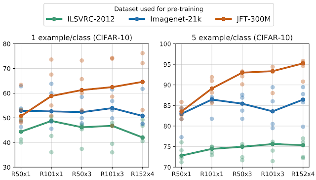
When transfering BiT to tasks with very few examples, we observe that as we simultaneously increase the amount of generic data used for pre-training and the architecture capacity, the ability of the resulting model to adapt to novel data drastically improves. On both 1-shot and 5-shot CIFAR (see Fig below) increasing model capacity yields limited returns when pre-training on ILSVRC (green curves). Yet, with large-scale pre-training on JFT, each step-up in model capacity yields massive returns (brown curves), up to BiT-L which attains 64% 1-shot and 95% 5-shot.
The curves depict median accuracy over 5 independent runs (light points) when transferring to CIFAR-10 with only 1 or 5 images per class (10 or 50 images total). It is evident that large architectures pre-trained on large datasets are significantly more data-efficient.
In order to verify that this result holds more generally, we also evaluate BiT on VTAB-1k, which is a suite of 19 diverse tasks with only 1000 labeled examples per task. We transfer the BiT-L model to all these tasks and achieve a score of 76.3% overall, which is a 5.8% absolute improvement over the previous state-of-the-art.

We show that this strategy of large-scale pre-training and simple transfer is effective even when a moderate amount of data is available by evaluating BiT-L on several standard computer vision benchmarks such as Oxford Pets and Flowers, CIFAR, etc. On all of these, BiT-L matches or surpasses state-of-the-art results. Finally, we use BiT as a backbone for RetinaNet on the MSCOCO-2017 detection task and confirm that even for such a structured output task, using large-scale pre-training helps considerably.
Left: Accuracy of BiT-L compared to the previous state-of-the-art general model on various standard computer vision benchmarks. Right: Results in average precision (AP) of using BiT as backbone for RetinaNet on MSCOCO-2017.
It is important to emphasize that across all the different downstream tasks we consider, we do not perform per-task hyper-parameter tuning and rely on the BiT-HyperRule. As we show in the paper, even better results can be achieved by tuning hyperparameters on sufficiently large validation data.

Evaluation on “Real-World” Images (ObjectNet)
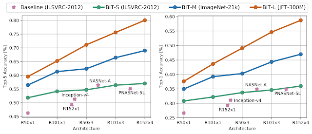
To further assess the robustness of BiT in a more challenging scenario, we evaluate BiT models that were fine-tuned on ILSVRC-2012 on the recently introduced ObjectNet dataset. This dataset closely resembles real-world scenarios, where objects may appear in atypical context, viewpoint, rotation, etc. Interestingly, the benefit from data and architecture scale is even more pronounced with the BiT-L model achieving unprecedented top-5 accuracy of 80.0%, an almost 25% absolute improvement over the previous state-of-the-art.
Results of BiT on the ObjectNet evaluation dataset. Left: top-5 accuracy, right: top-1 accuracy.
Conclusion
We show that given pre-training on large amounts of generic data, a simple transfer strategy leads to impressive results, both on large datasets as well as tasks with very little data, down to a single image per class. We release the BiT-M model, a R152x4 pre-trained on ImageNet-21k, along with colabs for transfer in Jax, TensorFlow2, and PyTorch. We hope that practitioners and researchers find it a useful alternative to commonly used ImageNet pre-trained models.

Acknowledgements
We would like to thank Xiaohua Zhai, Joan Puigcerver, Jessica Yung, Sylvain Gelly, and Neil Houlsby who have co-authored the BiT paper and been involved in all aspects of its development, as well as the Brain team in Zürich. We also would like to thank Andrei Giurgiu for his help in debugging input pipelines. We thank Tom Small for creating the animations used in this blogpost. Finally, we refer the interested reader to the related approaches in this direction by our colleagues in Google Research, Noisy Student, as well as Facebook Research’s highly relevant Exploring the Limits of Weakly Supervised Pretraining.

Source: Google AI Blog


Announcing the 7th Fine-Grained Visual Categorization Workshop


Fine-grained visual categorization refers to the problem of distinguishing between images of closely related entities, e.g., a monarch butterfly (Danaus plexippus) from a viceroy (Limenitis archippus). At the time of the first FGVC workshop in 2011, very few fine-grained datasets existed, and the ones that were available (e.g., the CUB dataset of 200 bird species, launched at that workshop) presented a formidable challenge to the leading classification algorithms of the time. Fast forward to 2020, and the computer vision landscape has undergone breathtaking changes. Deep learning based methods helped CUB-200-2011 accuracy rocket from 17% to 90% and fine-grained datasets have proliferated, with data arriving from a diverse array of institutions, such as art museums, apparel retailers, and cassava farms.

In order to help support even further progress in this field, we are excited to sponsor and co-organize the 7th Workshop on Fine-Grained Visual Categorization (FGVC7), which will take place as a virtual gathering on June 19, 2020, in conjunction with the IEEE conference on Computer Vision and Pattern Recognition (CVPR). We’re excited to highlight this year’s world-class lineup of fine-grained challenges, ranging from fruit tree disease prediction to fashion attributes, and we invite computer vision researchers from across the world to participate in the workshop.
The FGVC workshop at CVPR 2020 focuses on subordinate categories, including (from left to right) wildlife camera traps, plant pathology, birds, herbarium sheets, apparel, and museum artifacts.
Real-World Impact of the FGVC Challenges
In addition to pushing the frontier of fine-grained recognition on ever more challenging datasets, each FGVC workshop cycle provides opportunities for fostering new collaborations between researchers and practitioners. Some of the efforts from the FGVC workshop have made the leap into the hands of real world users.

The 2018 FGVC workshop hosted a Fungi challenge with data for 1,500 mushroom species provided by the Danish Mycological Society. When the competition concluded, the leaderboard was topped by a team from Czech Technical University and the University of West Bohemia.

The mycologists subsequently invited the Czech researchers for a visit to Copenhagen to explore further collaboration and field test a new workflow for collaborative machine learning research in biodiversity. This resulted in a jointly authored conference paper, a mushroom recognition app for Android and iOS, and an open access model published on TensorFlow Hub.
The Svampeatlas app for mushroom recognition is a result of a Danish-Czech collaboration spun out of the FGVC 2018 Fungi challenge. The underlying model is now published on TF Hub. Images used with permission of the Danish Mycological Society.
The iCassava Disease Challenge from 2019 mentioned above is another example of an FGVC team effort finding its way into the real world. In this challenge, Google researchers in Ghana collaborated with Makerere University and the National Crops Resources Research Institute (NaCRRI) to produce an annotated dataset of five cassava disease categories.
Examples of cassava leaf disease represented in the 2019 iCassava challenge.
The teams are testing a new model in the fields in Uganda with local farmers, and the model will be published on TFHub soon.

This Year’s Challenges
FGVC7 will feature six challenges, four of which represent sequels to past offerings, and two of which are brand new.

In iWildCam, the challenge is to identify different species of animals in camera trap images. Like its predecessors in 2018 and 2019, this year’s competition makes use of data from static, motion-triggered cameras used by biologists to study animals in the wild. Participants compete to build models that address diverse regions from around the globe, with a focus on generalization to held-out camera deployments within those regions, which exhibit differences in device model, image quality, local environment, lighting conditions, and species distributions, making generalization difficult.

It has been shown that species classification performance can be dramatically improved by using information beyond the image itself. In addition, since an ecosystem can be monitored in a variety of ways (e.g., camera traps, citizen scientists, remote sensing), each of which has its own strengths and limitations, it is important to facilitate the exploration of techniques for combining these complementary modalities. To this end, the competition provides a time series of remote sensing imagery for each camera trap location, as well as images from the iNaturalist competition datasets for species in the camera trap data.
Side-by-side comparison of image quality from iWildcam, captured from wildlife camera traps, (left) and iNaturalist (right), captured by conventional cameras. Images are from the 2020 iWildCam Challenge, and the iNaturalist competition datasets from 2017 and 2018.
The Herbarium Challenge, now in its second year, entails plant species identification, based on a large, long-tailed collection of herbarium specimens. Developed in collaboration with the New York Botanical Garden (NYBG), this challenge features over 1 million images representing over 32,000 plant species. Last year’s challenge was based on 46,000 specimens for 680 species. Being able to recognize species from historical herbarium collections can not only help botanists better understand changes in plant life on our planet, but also offers a unique opportunity to identify previously undescribed new species in the collection.
Representative examples of specimens from the 2020 Herbarium challenge. Images used with permission of the New York Botanical Garden.
In this year’s iMat Fashion challenge, participants compete to perform apparel instance segmentation and fine-grained attribute classification. The goal of this competition is to push the state of the art in fine-grained segmentation by joining forces between the fashion and computer vision communities. This challenge is in its third iteration, growing both in size and level of detail over past years’ offerings.

The last of the sequels is iMet, in which participants are challenged with building algorithms for fine-grained attribute classification on works of art. Developed in collaboration with the Metropolitan Museum of Art, the dataset has grown significantly since the 2019 edition, with a wide array of new cataloguing information generated by subject matter experts including multiple object classifications, artist, title, period, date, medium, culture, size, provenance, geographic location, and other related museum objects within the Met’s collection.

Semi-Supervised Aves is one of the new challenges at this year’s workshop. While avian data from iNaturalist has featured prominently in past FGVC challenges, this challenge focuses on the problem of learning from partially labeled data, a form of semi-supervised learning. The dataset is designed to expose some of the challenges encountered in realistic settings, such as the fine-grained similarity between classes, significant class imbalance, and domain mismatch between the labeled and unlabeled data.

Rounding out the set of challenges is Plant Pathology. In this challenge, the participants attempt to spot foliar diseases of apples using a reference dataset of expert-annotated diseased specimens. While this particular challenge is new to the FGVC community, it is the second such challenge to involve plant disease, the first being iCassava at last year’s FGVC.

Invitation to Participate
The results of these competitions will be presented at the FGVC7 workshop by top performing teams. We invite researchers, practitioners, and domain experts to participate in the FGVC workshop to learn more about state-of-the-art advances in fine-grained image recognition. We are excited to encourage the community's development of cutting edge algorithms for fine-grained visual categorization and foster new collaborations with global impact!

Acknowledgements
We’d like to thank our colleagues and friends on the FGVC7 organizing committee for working together to advance this important area. At Google we would like to thank Hartwig Adam, Kiat Chuan Tan, Arvi Gjoka, Kimberly Wilber, Sara Beery, Mikhail Sirotenko, Denis Brulé, Timnit Gebru, Ernest Mwebaze, Wojciech Sirko, Maggie Demkin.

Source: Google AI Blog


EfficientDet: Towards Scalable and Efficient Object Detection


As one of the core applications in computer vision, object detection has become increasingly important in scenarios that demand high accuracy, but have limited computational resources, such as robotics and driverless cars. Unfortunately, many current high-accuracy detectors do not fit these constraints. More importantly, real-world applications of object detection are run on a variety of platforms, which often demand different resources. A natural question, then, is how to design accurate and efficient object detectors that can also adapt to a wide range of resource constraints?

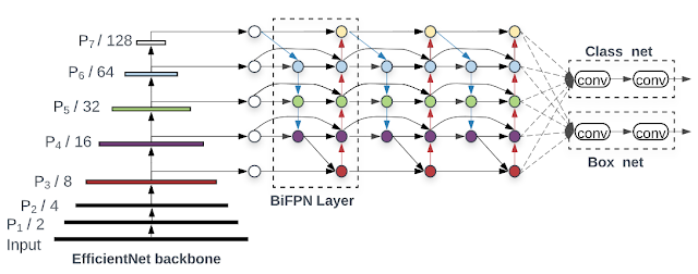
In “EfficientDet: Scalable and Efficient Object Detection”, accepted at CVPR 2020, we introduce a new family of scalable and efficient object detectors. Building upon our previous work on scaling neural networks (EfficientNet), and incorporating a novel bi-directional feature network (BiFPN) and new scaling rules, EfficientDet achieves state-of-the-art accuracy while being up to 9x smaller and using significantly less computation compared to prior state-of-the-art detectors. The following figure shows the overall network architecture of our models.
EfficientDet architecture. EfficientDet uses EfficientNet as the backbone network and a newly proposed BiFPN feature network.
Model Architecture Optimizations
The idea behind EfficientDet arose from our effort to find solutions to improve computational efficiency by conducting a systematic study of prior state-of-the-art detection models. In general, object detectors have three main components: a backbone that extracts features from the given image; a feature network that takes multiple levels of features from the backbone as input and outputs a list of fused features that represent salient characteristics of the image; and the final class/box network that uses the fused features to predict the class and location of each object. By examining the design choices for these components, we identified several key optimizations to improve performance and efficiency:

Previous detectors mainly rely on ResNets, ResNeXt, or AmoebaNet as backbone networks, which are all either less powerful or have lower efficiency than EfficientNets. By first implementing an EfficientNet backbone, it is possible to achieve much better efficiency. For example, starting from a RetinaNet baseline that employs ResNet-50 backbone, our ablation study shows that simply replacing ResNet-50 with EfficientNet-B3 can improve accuracy by 3% while reducing computation by 20%.

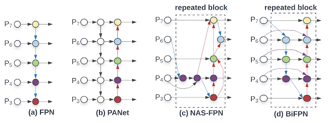
Another optimization is to improve the efficiency of the feature networks. While most previous detectors simply employ a top-down feature pyramid network (FPN), we find top-down FPN is inherently limited by the one-way information flow. Alternative FPNs, such as PANet, add an additional bottom-up flow at the cost of more computation. Recent efforts to leverage neural architecture search (NAS) discovered the more complex NAS-FPN architecture. However, while this network structure is effective, it is also irregular and highly optimized for a specific task, which makes it difficult to adapt to other tasks.

To address these issues, we propose a new bi-directional feature network, BiFPN, which incorporates the multi-level feature fusion idea from FPN/PANet/NAS-FPN that enables information to flow in both the top-down and bottom-up directions, while using regular and efficient connections.
A comparison between our BiFPN and previous feature networks. Our BiFPN allows features (from the low resolution P3 levels to high-resolution P7 levels) to repeatedly flow in both top-down and bottom-up ways.
To improve the efficiency even more, we propose a new fast normalized fusion technique. Traditional approaches usually treat all features input to the FPN equally, even those with different resolutions. However, we observe that input features at different resolutions often have unequal contributions to the output features. Thus, we add an additional weight for each input feature and allow the network to learn the importance of each. We also replace all regular convolutions with less expensive depthwise separable convolutions. With these optimizations, our BiFPN further improves the accuracy by 4%, while reducing the computation cost by 50%.

A third optimization involves achieving better accuracy and efficiency trade-offs under different resource constraints. Our previous work has shown that jointly scaling the depth, width and resolution of a network can significantly improve efficiency for image recognition. Inspired by this idea, we propose a new compound scaling method for object detectors, which jointly scales up the resolution/depth/width. Each network component, i.e., backbone, feature, and box/class prediction network, will have a single compound scaling factor that controls all scaling dimensions using heuristic-based rules. This approach enables one to easily determine how to scale the model by computing the scaling factor for the given target resource constraints.

Combining the new backbone and BiFPN, we first develop a small-size EfficientDet-D0 baseline, and then apply a compound scaling to obtain EfficientDet-D1 to D7. Each consecutive model has a higher compute cost, covering a wide range of resource constraints from 3 billion FLOPs to 300 billion FLOPS, and provides higher accuracy.

Model Performance
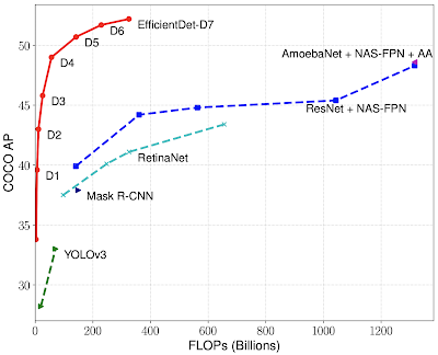
We evaluate EfficientDet on the COCO dataset, a widely used benchmark dataset for object detection. EfficientDet-D7 achieves a mean average precision (mAP) of 52.2, exceeding the prior state-of-the-art model by 1.5 points, while using 4x fewer parameters and 9.4x less computation.
EfficientDet achieves state-of-the-art 52.2 mAP, up 1.5 points from the prior state of the art (not shown since it is at 3045B FLOPs) on COCO test-dev under the same setting. Under the same accuracy constraint, EfficientDet models are 4x-9x smaller and use 13x-42x less computation than previous detectors.
We have also compared the parameter size and CPU/GPU latency between EfficientDet and previous models. Under similar accuracy constraints, EfficientDet models are 2x-4x faster on GPU, and 5x-11x faster on CPU than other detectors.

While the EfficientDet models are mainly designed for object detection, we also examine their performance on other tasks, such as semantic segmentation. To perform segmentation tasks, we slightly modify EfficientDet-D4 by replacing the detection head and loss function with a segmentation head and loss, while keeping the same scaled backbone and BiFPN. We compare this model with prior state-of-the-art segmentation models for Pascal VOC 2012, a widely used dataset for segmentation benchmark.
EfficientDet achieves better quality on Pascal VOC 2012 val than DeepLabV3+ with 9.8x less computation, under the same setting without COCO pre-training.
Open Source
Given their exceptional performance, we expect EfficientDet could serve as a new foundation of future object detection related research, and potentially make high-accuracy object detection models practically useful for many real-world applications. Therefore, we have open sourced all the code and pretrained model checkpoints on this github link.

Acknowledgements
Thanks to the paper co-authors Ruoming Pang and Quoc V. Le. We thank Daiyi Peng, Golnaz Ghiasi, Tianjian Meng for their help on infrastructure and discussion. We also thank Adam Kraft, Barret Zoph, Ekin D. Cubuk, Hongkun Yu, Jeff Dean, Pengchong Jin, Samy Bengio, Tsung-Yi Lin, Xianzhi Du, Xiaodan Song, and the Google Brain team.

Source: Google AI Blog


uDepth: Real-time 3D Depth Sensing on the Pixel 4


The ability to determine 3D information about the scene, called depth sensing, is a valuable tool for developers and users alike. Depth sensing is a very active area of computer vision research with recent innovations ranging from applications like portrait mode and AR to fundamental sensing innovations such as transparent object detection. Typical RGB-based stereo depth sensing techniques can be computationally expensive, suffer in regions with low texture, and fail completely in extreme low light conditions.

Because the Face Unlock feature on Pixel 4 must work at high speed and in darkness, it called for a different approach. To this end, the front of the Pixel 4 contains a real-time infrared (IR) active stereo depth sensor, called uDepth. A key computer vision capability on the Pixel 4, this technology helps the authentication system identify the user while also protecting against spoof attacks. It also supports a number of novel capabilities, such as after-the-fact photo retouching, depth-based segmentation of a scene, background blur, portrait effects and 3D photos.

Recently, we provided access to uDepth as an API on Camera2, using the Pixel Neural Core, two IR cameras, and an IR pattern projector to provide time-synchronized depth frames (in DEPTH16) at 30Hz. The Google Camera App uses this API to bring improved depth capabilities to selfies taken on the Pixel 4. In this post, we explain broadly how uDepth works, elaborate on the underlying algorithms, and discuss applications with example results for the Pixel 4.

Overview of Stereo Depth Sensing
All stereo camera systems reconstruct depth using parallax. To observe this effect, look at an object, close one eye, then switch which eye is closed. The apparent position of the object will shift, with closer objects appearing to move more. uDepth is part of the family of dense local stereo matching techniques, which estimate parallax computationally for each pixel. These techniques evaluate a region surrounding each pixel in the image formed by one camera, and try to find a similar region in the corresponding image from the second camera. When calibrated properly, the reconstructions generated are metric, meaning that they express real physical distances.
Pixel 4 front sensor setup, an example of an active stereo system.
To deal with textureless regions and cope with low-light conditions, we make use of an “active stereo” setup, which projects an IR pattern into the scene that is detected by stereo IR cameras. This approach makes low-texture regions easier to identify, improving results and reducing the computational requirements of the system.

What Makes uDepth Distinct?
Stereo sensing systems can be extremely computationally intensive, and it’s critical that a sensor running at 30Hz is low power while remaining high quality. uDepth leverages a number of key insights to accomplish this.

One such insight is that given a pair of regions that are similar to each other, most corresponding subsets of those regions are also similar. For example, given two 8x8 patches of pixels that are similar, it is very likely that the top-left 4x4 sub-region of each member of the pair is also similar. This informs the uDepth pipeline’s initialization procedure, which builds a pyramid of depth proposals by comparison of non-overlapping tiles in each image and selecting those most similar. This process starts with 1x1 tiles, and accumulates support hierarchically until an initial low-resolution depth map is generated.

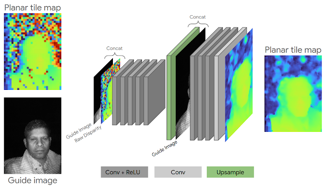
After initialization, we apply a novel technique for neural depth refinement to support the regular grid pattern illuminator on the Pixel 4. Typical active stereo systems project a pseudo-random grid pattern to help disambiguate matches in the scene, but uDepth is capable of supporting repeating grid patterns as well. Repeating structure in such patterns produces regions that look similar across stereo pairs, which can lead to incorrect matches. We mitigate this issue using a lightweight (75k parameter) convolutional architecture, using IR brightness and neighbor information to adjust incorrect matches — in less than 1.5ms per frame.
Neural depth refinement architecture.
Following neural depth refinement, good depth estimates are iteratively propagated from neighboring tiles. This and following pipeline steps leverage another insight key to the success of uDepth — natural scenes are typically locally planar with only small nonplanar deviations. This permits us to find planar tiles that cover the scene, and only later refine individual depths for each pixel in a tile, greatly reducing computational load.

Finally, the best match from among neighboring plane hypotheses is selected, with subpixel refinement and invalidation if no good match could be found.
Simplified depth architecture. Green components run on the GPU, yellow on the CPU, and blue on the Pixel Neural Core.
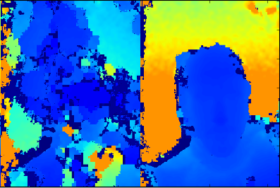
When a phone experiences a severe drop, it can result in the factory calibration of the stereo cameras diverging from the actual position of the cameras. To ensure high-quality results during real-world use, the uDepth system is self-calibrating. A scoring routine evaluates every depth image for signs of miscalibration, and builds up confidence in the state of the device. If miscalibration is detected, calibration parameters are regenerated from the current scene. This follows a pipeline consisting of feature detection and correspondence, subpixel refinement (taking advantage of the dot profile), and bundle adjustment.
Left: Stereo depth with inaccurate calibration. Right: After autocalibration.
For more details, please refer to Slanted O(1) Stereo, upon which uDepth is based.

Depth for Computational Photography
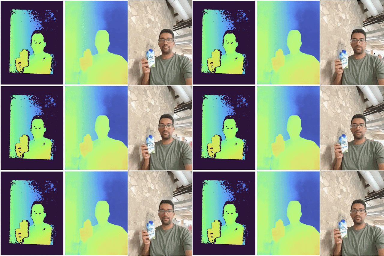
The raw data from the uDepth sensor is designed to be accurate and metric, which is a fundamental requirement for Face Unlock. Computational photography applications such as portrait mode and 3D photos have very different needs. In these use cases, it is not critical to achieve video frame rates, but the depth should be smooth, edge-aligned and complete in the whole field-of-view of the color camera.
Left to right: raw depth sensing result, predicted depth, 3D photo. Notice the smooth rotation of the wall, demonstrating a continuous depth gradient rather than a single focal plane.
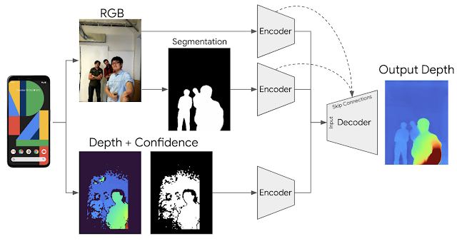
To achieve this we trained an end-to-end deep learning architecture that enhances the raw uDepth data, inferring a complete, dense 3D depth map. We use a combination of RGB images, people segmentation, and raw depth, with a dropout scheme forcing use of information for each of the inputs.
Architecture for computational photography depth enhancement.
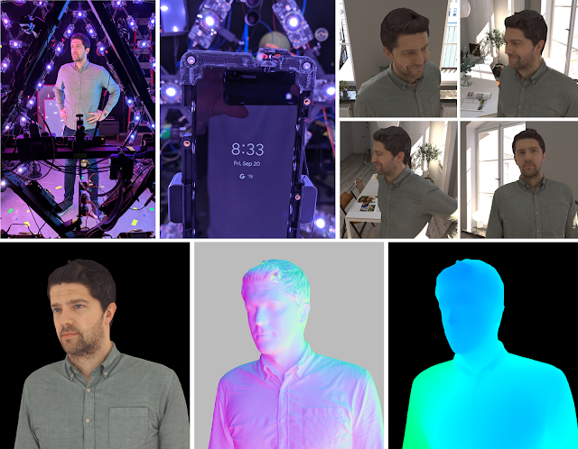
To acquire ground truth, we leveraged a volumetric capture system that can produce near-photorealistic models of people using a geodesic sphere outfitted with 331 custom color LED lights, an array of high-resolution cameras, and a set of custom high-resolution depth sensors. We added Pixel 4 phones to the setup and synchronized them with the rest of the hardware (lights and cameras). The generated training data consists of a combination of real images as well as synthetic renderings from the Pixel 4 camera viewpoint.
Data acquisition overview.
Putting It All Together
With all of these components in place, uDepth produces both a depth stream at 30Hz (exposed via Camera2), and smooth, post-processed depth maps for photography (exposed via Google Camera App when you take a depth-enabled selfie). The smooth, dense, per-pixel depth that our system produces is available on every Pixel 4 selfie with Social Media Depth features enabled, and can be used for post-capture effects such as bokeh and 3D photos for social media.
Example applications. Notice the multiple focal planes in the 3D photo on the right.
Finally, we are happy to provide a demo application for you to play with that visualizes a real-time point cloud from uDepth — download it here (this app is for demonstration and research purposes only and not intended for commercial use; Google will not provide any support or updates). This demo app visualizes 3D point clouds from your Pixel 4 device. Because the depth maps are time-synchronized and in the same coordinate system as the RGB images, a textured view of the 3D scene can be shown, as in the example visualization below:
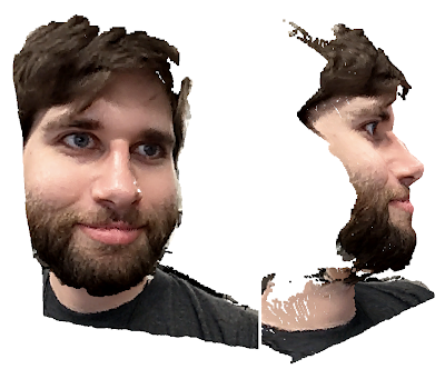
Example single-frame, RGB point cloud from uDepth on the Pixel 4.
Acknowledgements
This work would not have been possible without the contributions of many, many people, including but not limited to Peter Barnum, Cheng Wang, Matthias Kramm, Jack Arendt, Scott Chung, Vaibhav Gupta, Clayton Kimber, Jeremy Swerdlow, Vladimir Tankovich, Christian Haene, Yinda Zhang, Sergio Orts Escolano, Sean Ryan Fanello, Anton Mikhailov, Philippe Bouchilloux, Mirko Schmidt, Ruofei Du, Karen Zhu, Charlie Wang, Jonathan Taylor, Katrina Passarella, Eric Meisner, Vitalii Dziuba, Ed Chang, Phil Davidson, Rohit Pandey, Pavel Podlipensky, David Kim, Jay Busch, Cynthia Socorro Herrera, Matt Whalen, Peter Lincoln, Geoff Harvey, Christoph Rhemann, Zhijie Deng, Daniel Finchelstein, Jing Pu, Chih-Chung Chang, Eddy Hsu, Tian-yi Lin, Sam Chang, Isaac Christensen, Donghui Han, Speth Chang, Zhijun He, Gabriel Nava, Jana Ehmann, Yichang Shih, Chia-Kai Liang, Isaac Reynolds, Dillon Sharlet, Steven Johnson, Zalman Stern, Jiawen Chen, Ricardo Martin Brualla, Supreeth Achar, Mike Mehlman, Brandon Barbello, Chris Breithaupt, Michael Rosenfield, Gopal Parupudi, Steve Goldberg, Tim Knight, Raj Singh, Shahram Izadi, as well as many other colleagues across Devices and Services, Google Research, Android and X. 

Source: Google AI Blog


Announcing the 2020 Image Matching Benchmark and Challenge


Reconstructing 3D objects and buildings from a series of images is a well-known problem in computer vision, known as Structure-from-Motion (SfM). It has diverse applications in photography and cultural heritage preservation (e.g., allowing people to explore the sculptures of Rapa Nui in a browser) and powers many services across Google Maps, such as the 3D models created from StreetView and aerial imagery. In these examples, images are usually captured by operators under controlled conditions. While this ensures homogeneous data with a uniform, high-quality appearance in the images and the final reconstruction, it also limits the diversity of sites captured and the viewpoints from which they are seen. What if, instead of using images from tightly controlled conditions, one could apply SfM techniques to better capture the richness of the world using the vast amounts of unstructured image collections freely available on the internet?

In order to accelerate research into this topic, and how to better leverage the volume of data already publicly available, we present, “Image Matching across Wide Baselines: From Paper to Practice”, a collaboration with UVIC, CTU and EPFL, that presents a new public benchmark to evaluate methods for 3D reconstruction. Following on the results of the first Image Matching: Local Features and Beyond workshop held at CVPR 2019, this project now includes more than 25k images, each of which includes accurate pose information (location and orientation). This data is publicly available, along with the open-sourced benchmark, and is the foundation of the 2020 Image Matching Challenge to be held at CVPR 20201.

Recovering 3D Structure In the Wild
Google Maps already uses images donated by users to inform visitors about popular locations or to update business hours. However, using this type of data to build 3D models is much more difficult, since donated photos have a wide variety of viewpoints, lighting and weather conditions, occlusions from people and vehicles, and the occasional user-applied filters. The examples below highlight the diversity of images for the Trevi Fountain in Rome.
Some example images sampled from the Image Matching Challenge dataset, showing different perspectives of the Trevi Fountain.
In general, the use of SfM to reconstruct 3D scenes starts by identifying which parts of the images capture the same physical points of a scene, the corners of a window, for instance. This is achieved using local features, i.e., salient locations in an image that can be reliably identified across different views. They contain short description vectors (model representations) that capture the appearance around the point of interest. By comparing these descriptors, one can establish likely correspondences between the pixel coordinates of image locations across two or more images, and recover the 3D location of the point by triangulation. Both the pose from where the images were captured as well as the 3D location of the physical points observed (for example, identifying where the corner of the window is relative to the camera location) can then be jointly estimated. Doing this over many images and points allows one to obtain very detailed reconstructions.
A 3D reconstruction generated from over 3000 images, including those from the previous figure.
The challenge for this approach is the risk of having incorrect correspondences due, for example, to repeated structure such as the windows of the building, that may be very similar to each other, or transient elements that do not persist across images, such as the crowds admiring the Trevi Fountain. One way to filter these out is by reasoning about relations between correspondences using multiple images. An additional, even more powerful approach is to design better methods for identifying and isolating local features, for instance, by ignoring points on transient elements such as people. But to better understand the shortcomings of existing local feature algorithms for SfM and to provide insight into promising directions for future research, it is necessary to have a reliable benchmark to measure performance.

A Benchmark for Evaluating Local Features for 3D Reconstruction
Local features power many Google services, such as Image Search and product recognition in Google Lens, and are also used in mixed reality applications, like Google Maps' Live View, which relies on traditional, handcrafted local features. Designing better algorithms to identify and describe local features will lead to better performance overall.

Comparing the performance of local feature algorithms, however, has been difficult, because it is not obvious how to collect "ground-truth" data for this purpose. Some computer vision tasks rely on crowdsourcing: Google's OpenImages dataset labels "objects" with bounding boxes or pixel masks, by combining machine learning techniques with human annotators. This is not possible in this case, as it is not known what constitutes a "good" local feature a priori, making labelling infeasible. Additionally, existing benchmarks such as HPatches, are often small or limited to a narrow range of transformations, which can bias the evaluation.

What matters is the quality of the reconstruction, and that benchmarks reflect real-world scale and challenges in order to highlight opportunities for developing new approaches. To this end, we have created the Image Matching Benchmark, the first benchmark to include a large dataset of images for training and evaluation. The dataset includes more than 25k images (sourced from the public YFCC100m dataset), each of which has been augmented with accurate pose information (location and orientation). We obtain this "pseudo" ground-truth from large-scale SfM (100s-1000s of images, for each scene), which provides accurate and stable poses, and then run our evaluation on smaller subsets (10s of images), a much more difficult problem. This approach does not require expensive sensors or human labelling, and it provides better proxy metrics than previous benchmarks, which were restricted to small and homogenous datasets.
Visualizations from our benchmark. We show point-to-point matches generated by different local feature algorithms. Left to right: SIFT, HardNet, LogPolarDesc, R2D2. For details, please refer to our website.
We hope this benchmark, dataset and challenge helps advance the state of the art in 3D reconstruction with heterogeneous images. If you’re interested in participating in the challenge, please see the 2020 Image Matching Challenge website for more details.

Acknowledgements
The benchmark is joint work by Yuhe Jin and Kwang Moo Yi (University of Victoria), Anastasiia Mishchuk and Pascal Fua (EPFL), Dmytro Mishkin and Jiří Matas (Czech Technical University), and Eduard Trulls (Google). The CVPR workshop is co-organized by Vassileios Balntas (Scape Technologies/Facebook), Vincent Lepetit (Ecole des Ponts ParisTech), Dmytro Mishkin and Jiří Matas (Czech Technical University), Johannes Schönberger (Microsoft), Eduard Trulls (Google), and Kwang Moo Yi (University of Victoria).

1 Please note that as of April 2, 2020, CVPR is currently on track, despite the COVID-19 pandemic. Challenge information will be updated as the situation develops. Please see the 2020 Image Matching Challenge website for details.

Source: Google AI Blog


Visual Transfer Learning for Robotic Manipulation


The idea that robots can learn to directly perceive the affordances of actions on objects (i.e., what the robot can or cannot do with an object) is called affordance-based manipulation, explored in research on learning complex vision-based manipulation skills including grasping, pushing, and throwing. In these systems, affordances are represented as dense pixel-wise action-value maps that estimate how good it is for the robot to execute one of several predefined motions at each location. For example, given an RGB-D image, an affordance-based grasping model might infer grasping affordances per pixel with a convolutional neural network. The grasping affordance value at each pixel would represent the success rate of performing a corresponding motion primitive (e.g. grasping action), which would then be executed by the robot at the position with the highest value.
Overview of affordance-based manipulation.
For methods such as this, the ability to do more with less data is incredibly important, since data collection through physical trial and error can be both time consuming and expensive. However, recent discoveries in transfer learning have shown that visual feature representations learned from large-scale computer vision datasets can be reused for deep learning agents, enabling them to learn faster and generalize better in video games and simulated environments. If end-to-end affordance-based robot learning models that map from pixels to actions could similarly benefit from these visual representations, one could begin to leverage the vast amounts of labeled visual data that are now available in order to more efficiently learn useful skills for real-world interaction with less training.

In “Learning to See before Learning to Act: Visual Pre-training for Manipulation”, a collaboration with researchers from MIT to be presented at ICRA 2020, we investigate whether existing pre-trained deep learning visual feature representations can improve the efficiency of learning robotic manipulation tasks, like grasping objects. By studying how we can intelligently transfer neural network weights between vision models and affordance-based manipulation models, we can evaluate how different visual feature representations benefit the exploration process and enable robots to quickly acquire manipulation skills using different grippers. We present practical techniques to pre-train deep learning models, which enable robots to learn to pick and grasp arbitrary objects in unstructured settings in less than 10 minutes of trial and error.
Does first learning to see, improve the speed at which a robot can learn to act? In this project, we study ways in which we can transfer knowledge learned from computer vision tasks (left) to robot manipulation tasks (right).
Transfer Learning for Affordance-Based Manipulation
Affordance-based manipulation is essentially a way to reframe a manipulation task as a computer vision task, but rather than referencing pixels to object labels, we instead associate pixels to the value of actions. Since the structure of computer vision models and affordance models are so similar, one can leverage techniques from transfer learning in computer vision to enable affordance models to learn faster with less data. This approach re-purposes pre-trained neural network weights (i.e., feature representations) learned from large-scale vision datasets to initialize network weights of affordance models for robotic grasping.

In computer vision, many deep model architectures are composed of two parts: a “backbone” and a “head”. The backbone consists of weights that are responsible for early-stage image processing, e.g., filtering edges, detecting corners, and distinguishing between colors, while the head consists of network weights that are used in latter-stage processing, such as identifying high-level features, recognizing contextual cues, and executing spatial reasoning. The head is often much smaller than the backbone and is also more task specific. Hence, it is common practice in transfer learning to pre-train (e.g., on ResNet) and share backbone weights between tasks, while randomly initializing the weights of the model head for each new task.

Following this recipe, we initialized our affordance-based manipulation models with backbones based on the ResNet-50 architecture and pre-trained on different vision tasks, including a classification model from ImageNet and a segmentation model from COCO. With different initializations, the robot was then tasked with learning to grasp a diverse set of objects through trial and error.

Initially, we did not see any significant gains in performance compared with training from scratch – grasping success rates on training objects were only able to rise to 77% after 1,000 trial and error grasp attempts, outperforming training from scratch by 2%. However, upon transferring network weights from both the backbone and the head of the pre-trained COCO vision model, we saw a substantial improvement in training speed – grasping success rates reached 73% in just 500 trial and error grasp attempts, and jumped to 86% by 1,000 attempts. In addition, we tested our model on new objects unseen during training and found that models with the pre-trained backbone from COCO generalize better. The grasping success rates reach 83% with pre-trained backbone alone and further improve to 90% with both pre-trained backbone and head, outperforming the 46% reached by a model trained from scratch.
Affordance-based grasping models trained from scratch can struggle to pick up new objects after 60 minutes of training (left). With pre-training from visual tasks, our affordance-based grasping models can easily generalize to picking up new objects with less than 10 minutes of training, even when evaluated with different hardware (middle: suction, right: gripper).
Transfer Learning Can Improve Exploration
In our experiments with the grasping robot, we observed that the distribution of successful grasps versus failures in the generated datasets was far more balanced when network weights from both the backbone and head of pre-trained vision models were transferred to the affordance models, as opposed to only transferring the backbone.
Number of successful grasps out of the first 50 attempts using: a random initialization of weights, backbone and head pre-trained on ImageNet, COCO pre-trained backbone only, and backbone and head trained on COCO.
These results suggest that reusing network weights from vision tasks that require object localization (e.g., instance segmentation, like COCO) has the potential to significantly improve the exploration process when learning manipulation tasks. Pre-trained weights from these tasks encourage the robot to sample actions on things that look more like objects, thereby quickly generating a more balanced dataset from which the system can learn the differences between good and bad grasps. In contrast, pre-trained weights from vision tasks that potentially discard objects’ spatial information (e.g., image classification, like ImageNet) can only improve the performance slightly compared to random initialization.

To better understand this, we visualize the neural activations that are triggered by different pre-trained models and a converged affordance model trained from scratch using a suction gripper. Interestingly, we find that the intermediate network representations learned from the head of vision models used for segmentation from the COCO dataset activate on objects in ways that are similar to the converged affordance model. This aligns with the idea that transferring as much of the vision model as possible (both backbone and head) can lead to more object-centric exploration by leveraging model weights that are better at picking up visual features and localizing objects.
Affordances predicted by different models from images of cluttered objects (a). (b) Random refers to a randomly initialized model. (c) ImageNet is a model with backbone pre-trained on ImageNet and a randomly initialized head. (d) Normal refers to a model pre-trained to detect pixels with surface normals close to the anti-gravity axis. (e) COCO is the modified segmentation model (MaskRCNN) trained on the COCO dataset. (f) Suction is a converged model learned from robot-environment interactions using the suction gripper.
Limitations and Future Work
Many of the methods that we use today for end-to-end robot learning are effectively the same as those being used for computer vision tasks. Our work here on visual pre-training illuminates this connection and demonstrates that it is possible to leverage techniques from visual pre-training to improve the learning efficiency of affordance-base manipulation applied to robotic grasping tasks. While our experiments point to a better understanding of deep learning for robots, there are still many interesting questions that have yet to be explored. For example, how do we leverage large-scale pre-training for additional modes of sensing (e.g. force-torque or tactile)? How do we extend these pre-training techniques towards more complex manipulation tasks that may not be as object-centric as grasping? These areas are promising directions for future research.

You can learn more about this work in the summary video below.
Acknowledgements
This research was done by Yen-Chen Lin (Ph.D. student at MIT), Andy Zeng, Shuran Song, Phillip Isola (faculty at MIT), and Tsung-Yi Lin, with special thanks to Johnny Lee and Ivan Krasin for valuable managerial support, Chad Richards for helpful feedback on writing, and Jonathan Thompson for fruitful technical discussions.

Source: Google AI Blog


Real-Time 3D Object Detection on Mobile Devices with MediaPipe


Object detection is an extensively studied computer vision problem, but most of the research has focused on 2D object prediction. While 2D prediction only provides 2D bounding boxes, by extending prediction to 3D, one can capture an object’s size, position and orientation in the world, leading to a variety of applications in robotics, self-driving vehicles, image retrieval, and augmented reality. Although 2D object detection is relatively mature and has been widely used in the industry, 3D object detection from 2D imagery is a challenging problem, due to the lack of data and diversity of appearances and shapes of objects within a category.

Today, we are announcing the release of MediaPipe Objectron, a mobile real-time 3D object detection pipeline for everyday objects. This pipeline detects objects in 2D images, and estimates their poses and sizes through a machine learning (ML) model, trained on a newly created 3D dataset. Implemented in MediaPipe, an open-source cross-platform framework for building pipelines to process perceptual data of different modalities, Objectron computes oriented 3D bounding boxes of objects in real-time on mobile devices.
 
3D Object Detection from a single image. MediaPipe Objectron determines the position, orientation and size of everyday objects in real-time on mobile devices.
Obtaining Real-World 3D Training Data
While there are ample amounts of 3D data for street scenes, due to the popularity of research into self-driving cars that rely on 3D capture sensors like LIDAR, datasets with ground truth 3D annotations for more granular everyday objects are extremely limited. To overcome this problem, we developed a novel data pipeline using mobile augmented reality (AR) session data. With the arrival of ARCore and ARKit, hundreds of millions of smartphones now have AR capabilities and the ability to capture additional information during an AR session, including the camera pose, sparse 3D point clouds, estimated lighting, and planar surfaces.

In order to label ground truth data, we built a novel annotation tool for use with AR session data, which allows annotators to quickly label 3D bounding boxes for objects. This tool uses a split-screen view to display 2D video frames on which are overlaid 3D bounding boxes on the left, alongside a view showing 3D point clouds, camera positions and detected planes on the right. Annotators draw 3D bounding boxes in the 3D view, and verify its location by reviewing the projections in 2D video frames. For static objects, we only need to annotate an object in a single frame and propagate its location to all frames using the ground truth camera pose information from the AR session data, which makes the procedure highly efficient.
Real-world data annotation for 3D object detection. Right: 3D bounding boxes are annotated in the 3D world with detected surfaces and point clouds. Left: Projections of annotated 3D bounding boxes are overlaid on top of video frames making it easy to validate the annotation.
AR Synthetic Data Generation
A popular approach is to complement real-world data with synthetic data in order to increase the accuracy of prediction. However, attempts to do so often yield poor, unrealistic data or, in the case of photorealistic rendering, require significant effort and compute. Our novel approach, called AR Synthetic Data Generation, places virtual objects into scenes that have AR session data, which allows us to leverage camera poses, detected planar surfaces, and estimated lighting to generate placements that are physically probable and with lighting that matches the scene. This approach results in high-quality synthetic data with rendered objects that respect the scene geometry and fit seamlessly into real backgrounds. By combining real-world data and AR synthetic data, we are able to increase the accuracy by about 10%.
An example of AR synthetic data generation. The virtual white-brown cereal box is rendered into the real scene, next to the real blue book.
An ML Pipeline for 3D Object Detection
We built a single-stage model to predict the pose and physical size of an object from a single RGB image. The model backbone has an encoder-decoder architecture, built upon MobileNetv2. We employ a multi-task learning approach, jointly predicting an object's shape with detection and regression. The shape task predicts the object's shape signals depending on what ground truth annotation is available, e.g. segmentation. This is optional if there is no shape annotation in training data. For the detection task, we use the annotated bounding boxes and fit a Gaussian to the box, with center at the box centroid, and standard deviations proportional to the box size. The goal for detection is then to predict this distribution with its peak representing the object’s center location. The regression task estimates the 2D projections of the eight bounding box vertices. To obtain the final 3D coordinates for the bounding box, we leverage a well established pose estimation algorithm (EPnP). It can recover the 3D bounding box of an object, without a priori knowledge of the object dimensions. Given the 3D bounding box, we can easily compute pose and size of the object. The diagram below shows our network architecture and post-processing. The model is light enough to run real-time on mobile devices (at 26 FPS on an Adreno 650 mobile GPU).
Network architecture and post-processing for 3D object detection.
Sample results of our network — [left] original 2D image with estimated bounding boxes, [middle] object detection by Gaussian distribution, [right] predicted segmentation mask.
Detection and Tracking in MediaPipe
When the model is applied to every frame captured by the mobile device, it can suffer from jitter due to the ambiguity of the 3D bounding box estimated in each frame. To mitigate this, we adopt the detection+tracking framework recently released in our 2D object detection and tracking solution. This framework mitigates the need to run the network on every frame, allowing the use of heavier and therefore more accurate models, while keeping the pipeline real-time on mobile devices. It also retains object identity across frames and ensures that the prediction is temporally consistent, reducing the jitter.

For further efficiency in our mobile pipeline, we run our model inference only once every few frames. Next, we take the prediction and track it over time using the approach described in our previous blogs for instant motion tracking and Motion Stills. When a new prediction is made, we consolidate the detection result with the tracking result based on the area of overlap.

To encourage researchers and developers to experiment and prototype based on our pipeline, we are releasing our on-device ML pipeline in MediaPipe, including an end-to-end demo mobile application and our trained models for two categories: shoes and chairs. We hope that sharing our solution with the wide research and development community will stimulate new use cases, new applications, and new research efforts. In the future, we plan to scale our model to many more categories, and further improve our on-device performance.
   
Examples of our 3D object detection in the wild.
Acknowledgements
The research described in this post was done by Adel Ahmadyan, Tingbo Hou, Jianing Wei, Matthias Grundmann, Liangkai Zhang, Jiuqiang Tang, Chris McClanahan, Tyler Mullen, Buck Bourdon, Esha Uboweja, Mogan Shieh, Siarhei Kazakou, Ming Guang Yong, Chuo-Ling Chang, and James Bruce. We thank Aliaksandr Shyrokau and the annotation team for their diligence to high quality annotations.

Source: Google AI Blog