Tag Archives: Computer Vision

MediaPipe Holistic — Simultaneous Face, Hand and Pose Prediction, on Device

Real-time, simultaneous perception of human pose, face landmarks and hand tracking on mobile devices can enable a variety of impactful applications, such as fitness and sport analysis, gesture control and sign language recognition, augmented reality effects and more. MediaPipe, an open-source framework designed specifically for complex perception pipelines leveraging accelerated inference (e.g., GPU or CPU), already offers fast and accurate, yet separate, solutions for these tasks. Combining them all in real-time into a semantically consistent end-to-end solution is a uniquely difficult problem requiring simultaneous inference of multiple, dependent neural networks.

Today, we are excited to announce MediaPipe Holistic, a solution to this challenge that provides a novel state-of-the-art human pose topology that unlocks novel use cases. MediaPipe Holistic consists of a new pipeline with optimized pose, face and hand components that each run in real-time, with minimum memory transfer between their inference backends, and added support for interchangeability of the three components, depending on the quality/speed tradeoffs. When including all three components, MediaPipe Holistic provides a unified topology for a groundbreaking 540+ keypoints (33 pose, 21 per-hand and 468 facial landmarks) and achieves near real-time performance on mobile devices. MediaPipe Holistic is being released as part of MediaPipe and is available on-device for mobile (Android, iOS) and desktop. We are also introducing MediaPipe’s new ready-to-use APIs for research (Python) and web (JavaScript) to ease access to the technology.

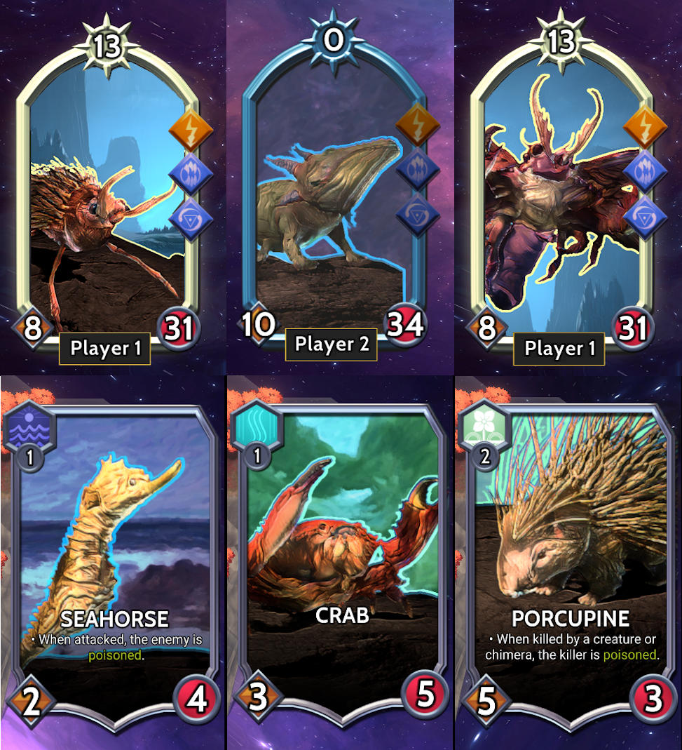
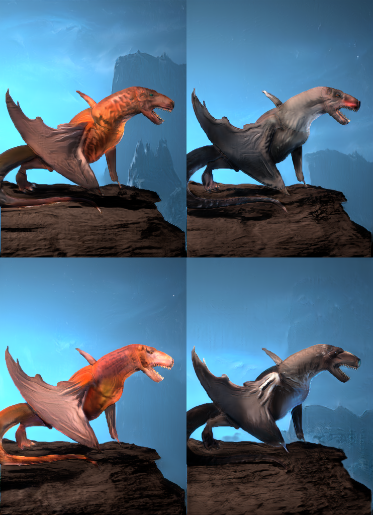
Top: MediaPipe Holistic results on sport and dance use-cases. Bottom: “Silence” and “Hello” gestures. Note, that our solution consistently identifies a hand as either right (blue color) or left (orange color).

Pipeline and Quality
The MediaPipe Holistic pipeline integrates separate models for pose, face and hand components, each of which are optimized for their particular domain. However, because of their different specializations, the input to one component is not well-suited for the others. The pose estimation model, for example, takes a lower, fixed resolution video frame (256x256) as input. But if one were to crop the hand and face regions from that image to pass to their respective models, the image resolution would be too low for accurate articulation. Therefore, we designed MediaPipe Holistic as a multi-stage pipeline, which treats the different regions using a region appropriate image resolution.

First, MediaPipe Holistic estimates the human pose with BlazePose’s pose detector and subsequent keypoint model. Then, using the inferred pose key points, it derives three regions of interest (ROI) crops for each hand (2x) and the face, and employs a re-crop model to improve the ROI (details below). The pipeline then crops the full-resolution input frame to these ROIs and applies task-specific face and hand models to estimate their corresponding keypoints. Finally, all key points are merged with those of the pose model to yield the full 540+ keypoints.

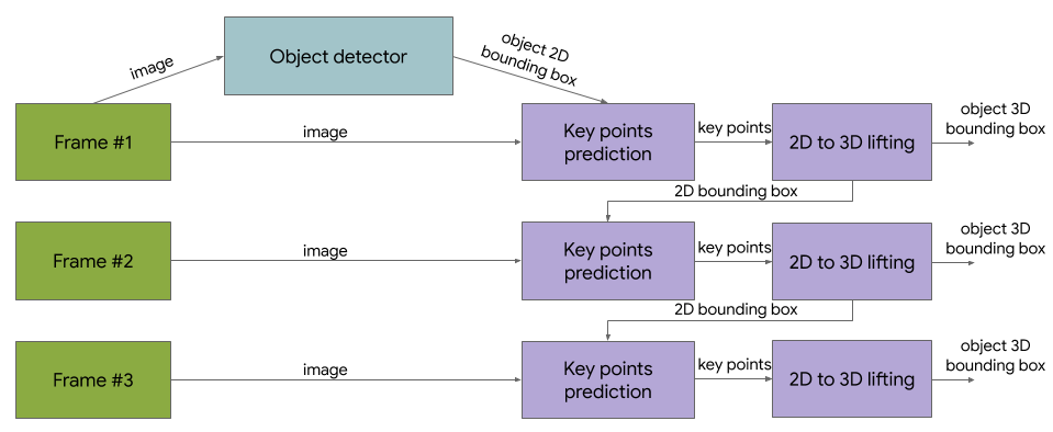
MediaPipe Holistic pipeline overview.

To streamline the identification of ROIs, a tracking approach similar to the one used for the standalone face and hand pipelines is utilized. This approach assumes that the object doesn't move significantly between frames, using an estimation from the previous frame as a guide to the object region in the current one. However, during fast movements, the tracker can lose the target, which requires the detector to re-localize it in the image. MediaPipe Holistic uses pose prediction (on every frame) as an additional ROI prior to reduce the response time of the pipeline when reacting to fast movements. This also enables the model to retain semantic consistency across the body and its parts by preventing a mixup between left and right hands or body parts of one person in the frame with another.

In addition, the resolution of the input frame to the pose model is low enough that the resulting ROIs for face and hands are still too inaccurate to guide the re-cropping of those regions, which require a precise input crop to remain lightweight. To close this accuracy gap we use lightweight face and hand re-crop models that play the role of spatial transformers and cost only ~10% of the corresponding model's inference time.

 MEH   FLE 
 Tracking pipeline (baseline)   9.8%   3.1% 
 Pipeline without re-crops   11.8%   3.5% 
 Pipeline with re-crops   9.7%   3.1% 
Hand prediction quality.The mean error per hand (MEH) is normalized by the hand size. The face landmarks error (FLE) is normalized by the inter-pupillary distance.

Performance
MediaPipe Holistic requires coordination between up to 8 models per frame — 1 pose detector, 1 pose landmark model, 3 re-crop models and 3 keypoint models for hands and face. While building this solution, we optimized not only machine learning models, but also pre- and post-processing algorithms (e.g., affine transformations), which take significant time on most devices due to pipeline complexity. In this case, moving all the pre-processing computations to GPU resulted in ~1.5 times overall pipeline speedup depending on the device. As a result, MediaPipe Holistic runs in near real-time performance even on mid-tier devices and in the browser.

 Phone   FPS 
 Google Pixel 2 XL   18 
 Samsung S9+   20 
 15-inch MacBook Pro 2017   15 
Performance on various mid-tier devices, measured in frames per second (FPS) using TFLite GPU.

The multi-stage nature of the pipeline provides two more performance benefits. As models are mostly independent, they can be replaced with lighter or heavier versions (or turned off completely) depending on the performance and accuracy requirements. Also, once pose is inferred, one knows precisely whether hands and face are within the frame bounds, allowing the pipeline to skip inference on those body parts.

Applications
MediaPipe Holistic, with its 540+ key points, aims to enable a holistic, simultaneous perception of body language, gesture and facial expressions. Its blended approach enables remote gesture interfaces, as well as full-body AR, sports analytics, and sign language recognition. To demonstrate the quality and performance of the MediaPipe Holistic, we built a simple remote control interface that runs locally in the browser and enables a compelling user interaction, no mouse or keyboard required. The user can manipulate objects on the screen, type on a virtual keyboard while sitting on the sofa, and point to or touch specific face regions (e.g., mute or turn off the camera). Underneath it relies on accurate hand detection with subsequent gesture recognition mapped to a "trackpad" space anchored to the user’s shoulder, enabling remote control from up to 4 meters.

This technique for gesture control can unlock various novel use-cases when other human-computer interaction modalities are not convenient. Try it out in our web demo and prototype your own ideas with it.

In-browser touchless control demos. Left: Palm picker, touch interface, keyboard. Right: Distant touchless keyboard. Try it out!

MediaPipe for Research and Web
To accelerate ML research as well as its adoption in the web developer community, MediaPipe now offers ready-to-use, yet customizable ML solutions in Python and in JavaScript. We are starting with those in our previous publications: Face Mesh, Hands and Pose, including MediaPipe Holistic, with many more to come. Try them directly in the web browser: for Python using the notebooks in MediaPipe on Google Colab, and for JavaScript with your own webcam input in MediaPipe on CodePen!

Conclusion
We hope the release of MediaPipe Holistic will inspire the research and development community members to build new unique applications. We anticipate that these pipelines will open up avenues for future research into challenging domains, such as sign-language recognition, touchless control interfaces, or other complex use cases. We are looking forward to seeing what you can build with it!

Complex and dynamic hand gestures. Videos by Dr. Bill Vicars, used with permission.

Acknowledgments
Special thanks to all our team members who worked on the tech with us: Fan Zhang, Gregory Karpiak, Kanstantsin Sokal, Juhyun Lee, Hadon Nash, Chuo-Ling Chang, Jiuqiang Tang, Nikolay Chirkov, Camillo Lugaresi, George Sung, Michael Hays, Tyler Mullen, Chris McClanahan, Ekaterina Ignasheva, Marat Dukhan, Artsiom Ablavatski, Yury Kartynnik, Karthik Raveendran, Andrei Vakunov, Andrei Tkachenka, Suril Shah, Buck Bourdon, Ming Guang Yong, Esha Uboweja, Siarhei Kazakou, Andrei Kulik, Matsvei Zhdanovich, and Matthias Grundmann.

Source: Google AI Blog


Transformers for Image Recognition at Scale

While convolutional neural networks (CNNs) have been used in computer vision since the 1980s, they were not at the forefront until 2012 when AlexNet surpassed the performance of contemporary state-of-the-art image recognition methods by a large margin. Two factors helped enable this breakthrough: (i) the availability of training sets like ImageNet, and (ii) the use of commoditized GPU hardware, which provided significantly more compute for training. As such, since 2012, CNNs have become the go-to model for vision tasks.

The benefit of using CNNs was that they avoided the need for hand-designed visual features, instead learning to perform tasks directly from data “end to end”. However, while CNNs avoid hand-crafted feature-extraction, the architecture itself is designed specifically for images and can be computationally demanding. Looking forward to the next generation of scalable vision models, one might ask whether this domain-specific design is necessary, or if one could successfully leverage more domain agnostic and computationally efficient architectures to achieve state-of-the-art results.

As a first step in this direction, we present the Vision Transformer (ViT), a vision model based as closely as possible on the Transformer architecture originally designed for text-based tasks. ViT represents an input image as a sequence of image patches, similar to the sequence of word embeddings used when applying Transformers to text, and directly predicts class labels for the image. ViT demonstrates excellent performance when trained on sufficient data, outperforming a comparable state-of-the-art CNN with four times fewer computational resources. To foster additional research in this area, we have open-sourced both the code and models.

The Vision Transformer treats an input image as a sequence of patches, akin to a series of word embeddings generated by a natural language processing (NLP) Transformer.

The Vision Transformer
The original text Transformer takes as input a sequence of words, which it then uses for classification, translation, or other NLP tasks. For ViT, we make the fewest possible modifications to the Transformer design to make it operate directly on images instead of words, and observe how much about image structure the model can learn on its own.

ViT divides an image into a grid of square patches. Each patch is flattened into a single vector by concatenating the channels of all pixels in a patch and then linearly projecting it to the desired input dimension. Because Transformers are agnostic to the structure of the input elements we add learnable position embeddings to each patch, which allow the model to learn about the structure of the images. A priori, ViT does not know about the relative location of patches in the image, or even that the image has a 2D structure — it must learn such relevant information from the training data and encode structural information in the position embeddings.

Scaling Up

We first train ViT on ImageNet, where it achieves a best score of 77.9% top-1 accuracy. While this is decent for a first attempt, it falls far short of the state of the art — the current best CNN trained on ImageNet with no extra data reaches 85.8%. Despite mitigation strategies (e.g., regularization), ViT overfits the ImageNet task due to its lack of inbuilt knowledge about images.

To investigate the impact of dataset size on model performance, we train ViT on ImageNet-21k (14M images, 21k classes) and JFT (300M images, 18k classes), and compare the results to a state-of-the-art CNN, Big Transfer (BiT), trained on the same datasets. As previously observed, ViT performs significantly worse than the CNN equivalent (BiT) when trained on ImageNet (1M images). However, on ImageNet-21k (14M images) performance is comparable, and on JFT (300M images), ViT now outperforms BiT.

Finally, we investigate the impact of the amount of computation involved in training the models. For this, we train several different ViT models and CNNs on JFT. These models span a range of model sizes and training durations. As a result, they require varying amounts of compute for training. We observe that, for a given amount of compute, ViT yields better performance than the equivalent CNNs.

Left: Performance of ViT when pre-trained on different datasets. Right: ViT yields a good performance/compute trade-off.

High-Performing Large-Scale Image Recognition
Our data suggest that (1) with sufficient training ViT can perform very well, and (2) ViT yields an excellent performance/compute trade-off at both smaller and larger compute scales. Therefore, to see if performance improvements carried over to even larger scales, we trained a 600M-parameter ViT model.

This large ViT model attains state-of-the-art performance on multiple popular benchmarks, including 88.55% top-1 accuracy on ImageNet and 99.50% on CIFAR-10. ViT also performs well on the cleaned-up version of the ImageNet evaluations set “ImageNet-Real”, attaining 90.72% top-1 accuracy. Finally, ViT works well on diverse tasks, even with few training data points. For example, on the VTAB-1k suite (19 tasks with 1,000 data points each), ViT attains 77.63%, significantly ahead of the single-model state of the art (SOTA) (76.3%), and even matching SOTA attained by an ensemble of multiple models (77.6%). Most importantly, these results are obtained using fewer compute resources compared to previous SOTA CNNs, e.g., 4x fewer than the pre-trained BiT models.

Vision Transformer matches or outperforms state-of-the-art CNNs on popular benchmarks. Left: Popular image classification tasks (ImageNet, including new validation labels ReaL, and CIFAR, Pets, and Flowers). Right: Average across 19 tasks in the VTAB classification suite.

Visualizations
To gain some intuition into what the model learns, we visualize some of its internal workings. First, we look at the position embeddings — parameters that the model learns to encode the relative location of patches — and find that ViT is able to reproduce an intuitive image structure. Each position embedding is most similar to others in the same row and column, indicating that the model has recovered the grid structure of the original images. Second, we examine the average spatial distance between one element attending to another for each transformer block. At higher layers (depths of 10-20) only global features are used (i.e., large attention distances), but the lower layers (depths 0-5) capture both global and local features, as indicated by a large range in the mean attention distance. By contrast, only local features are present in the lower layers of a CNN. These experiments indicate that ViT can learn features hard-coded into CNNs (such as awareness of grid structure), but is also free to learn more generic patterns, such as a mix of local and global features at lower layers, that can aid generalization.

Left: ViT learns the grid like structure of the image patches via its position embeddings. Right: The lower layers of ViT contain both global and local features, the higher layers contain only global features.

Summary
While CNNs have revolutionized computer vision, our results indicate that models tailor-made for imaging tasks may be unnecessary, or even sub-optimal. With ever-increasing dataset sizes, and the continued development of unsupervised and semi-supervised methods, the development of new vision architectures that train more efficiently on these datasets becomes increasingly important. We believe ViT is a preliminary step towards generic, scalable architectures that can solve many vision tasks, or even tasks from many domains, and are excited for future developments.

A preprint of our work as well as code and models are publically available.

Acknowledgements
We would like to thank our co-authors in Berlin, Zürich, and Amsterdam: Alexey Dosovitskiy, Lucas Beyer, Alexander Kolesnikov, Xiaohua Zhai, Thomas Unterthiner, Mostafa Dehghani, Matthias Minderer, Georg Heigold, Sylvain Gelly, and Jakob Uszkoreit. We would like to thank Andreas Steiner for crucial help with infrastructure and open-sourcing, Joan Puigcerver and Maxim Neumann for work on large-scale training infrastructure, and Dmitry Lepikhin, Aravindh Mahendran, Daniel Keysers, Mario Lučić, Noam Shazeer, and Colin Raffel for useful discussions. Finally, we thank Tom Small for creating the Visual Transformer animation in this post.

Source: Google AI Blog


Using GANs to Create Fantastical Creatures

Creating art for digital video games takes a high degree of artistic creativity and technical knowledge, while also requiring game artists to quickly iterate on ideas and produce a high volume of assets, often in the face of tight deadlines. What if artists had a paintbrush that acted less like a tool and more like an assistant? A machine learning model acting as such a paintbrush could reduce the amount of time necessary to create high-quality art without sacrificing artistic choices, perhaps even enhancing creativity.

Today, we present Chimera Painter, a trained machine learning (ML) model that automatically creates a fully fleshed out rendering from a user-supplied creature outline. Employed as a demo application, Chimera Painter adds features and textures to a creature outline segmented with body part labels, such as “wings” or “claws”, when the user clicks the “transform” button. Below is an example using the demo with one of the preset creature outlines.

Using an image imported to Chimera Painter or generated with the tools provided, an artist can iteratively construct or modify a creature outline and use the ML model to generate realistic looking surface textures. In this example, an artist (Lee Dotson) customizes one of the creature designs that comes pre-loaded in the Chimera Painter demo.

In this post, we describe some of the challenges in creating the ML model behind Chimera Painter and demonstrate how one might use the tool for the creation of video game-ready assets.

Prototyping for a New Type of Model
In developing an ML model to produce video-game ready creature images, we created a digital card game prototype around the concept of combining creatures into new hybrids that can then battle each other. In this game, a player would begin with cards of real-world animals (e.g., an axolotl or a whale) and could make them more powerful by combining them (making the dreaded Axolotl-Whale chimera). This provided a creative environment for demonstrating an image-generating model, as the number of possible chimeras necessitated a method for quickly designing large volumes of artistic assets that could be combined naturally, while still retaining identifiable visual characteristics of the original creatures.

Since our goal was to create high-quality creature card images guided by artist input, we experimented with generative adversarial networks (GANs), informed by artist feedback, to create creature images that would be appropriate for our fantasy card game prototype. GANs pair two convolutional neural networks against each other: a generator network to create new images and a discriminator network to determine if these images are samples from the training dataset (in this case, artist-created images) or not. We used a variant called a conditional GAN, where the generator takes a separate input to guide the image generation process. Interestingly, our approach was a strict departure from other GAN efforts, which typically focus on photorealism.

To train the GANs, we created a dataset of full color images with single-species creature outlines adapted from 3D creature models. The creature outlines characterized the shape and size of each creature, and provided a segmentation map that identified individual body parts. After model training, the model was tasked with generating multi-species chimeras, based on outlines provided by artists. The best performing model was then incorporated into Chimera Painter. Below we show some sample assets generated using the model, including single-species creatures, as well as the more complex multi-species chimeras.

Generated card art integrated into the card game prototype showing basic creatures (bottom row) and chimeras from multiple creatures, including an Antlion-Porcupine, Axolotl-Whale, and a Crab-Antion-Moth (top row). More info about the game itself is detailed in this Stadia Research presentation.

Learning to Generate Creatures with Structure
An issue with using GANs for generating creatures was the potential for loss of anatomical and spatial coherence when rendering subtle or low-contrast parts of images, despite these being of high perceptual importance to humans. Examples of this can include eyes, fingers, or even distinguishing between overlapping body parts with similar textures (see the affectionately named BoggleDog below).

GAN-generated image showing mismatched body parts.

Generating chimeras required a new non-photographic fantasy-styled dataset with unique characteristics, such as dramatic perspective, composition, and lighting. Existing repositories of illustrations were not appropriate to use as datasets for training an ML model, because they may be subject to licensing restrictions, have conflicting styles, or simply lack the variety needed for this task.

To solve this, we developed a new artist-led, semi-automated approach for creating an ML training dataset from 3D creature models, which allowed us to work at scale and rapidly iterate as needed. In this process, artists would create or obtain a set of 3D creature models, one for each creature type needed (such as hyenas or lions). Artists then produced two sets of textures that were overlaid on the 3D model using the Unreal Engine — one with the full color texture (left image, below) and the other with flat colors for each body part (e.g., head, ears, neck, etc), called a “segmentation map” (right image, below). This second set of body part segments was given to the model at training to ensure that the GAN learned about body part-specific structure, shapes, textures, and proportions for a variety of creatures.

Example dataset training image and its paired segmentation map.

The 3D creature models were all placed in a simple 3D scene, again using the Unreal Engine. A set of automated scripts would then take this 3D scene and interpolate between different poses, viewpoints, and zoom levels for each of the 3D creature models, creating the full color images and segmentation maps that formed the training dataset for the GAN. Using this approach, we generated 10,000+ image + segmentation map pairs per 3D creature model, saving the artists millions of hours of time compared to creating such data manually (at approximately 20 minutes per image).

Fine Tuning
The GAN had many different hyper-parameters that could be adjusted, leading to different qualities in the output images. In order to better understand which versions of the model were better than others, artists were provided samples for different creature types generated by these models and asked to cull them down to a few best examples. We gathered feedback about desired characteristics present in these examples, such as a feeling of depth, style with regard to creature textures, and realism of faces and eyes. This information was used both to train new versions of the model and, after the model had generated hundreds of thousands of creature images, to select the best image from each creature category (e.g., gazelle, lynx, gorilla, etc).

We tuned the GAN for this task by focusing on the perceptual loss. This loss function component (also used in Stadia’s Style Transfer ML) computes a difference between two images using extracted features from a separate convolutional neural network (CNN) that was previously trained on millions of photographs from the ImageNet dataset. The features are extracted from different layers of the CNN and a weight is applied to each, which affects their contribution to the final loss value. We discovered that these weights were critically important in determining what a final generated image would look like. Below are some examples from the GAN trained with different perceptual loss weights.

Dino-Bat Chimeras generated using varying perceptual loss weights.

Some of the variation in the images above is due to the fact that the dataset includes multiple textures for each creature (for example, a reddish or grayish version of the bat). However, ignoring the coloration, many differences are directly tied to changes in perceptual loss values. In particular, we found that certain values brought out sharper facial features (e.g., bottom right vs. top right) or “smooth” versus “patterned” (top right vs. bottom left) that made generated creatures feel more real.

Here are some creatures generated from the GAN trained with different perceptual loss weights, showing off a small sample of the outputs and poses that the model can handle.

Creatures generated using different models.
A generated chimera (Dino-Bat-Hyena, to be exact) created using the conditional GAN. Output from the GAN (left) and the post-processed / composited card (right).

Chimera Painter
The trained GAN is now available in the Chimera Painter demo, allowing artists to work iteratively with the model, rather than drawing dozens of similar creatures from scratch. An artist can select a starting point and then adjust the shape, type, or placement of creature parts, enabling rapid exploration and for the creation of a large volume of images. The demo also allows for uploading a creature outline created in an external program, like Photoshop. Simply download one of the preset creature outlines to get the colors needed for each creature part and use this as a template for drawing one outside of Chimera Painter, and then use the “Load’ button on the demo to use this outline to flesh out your creation.

It is our hope that these GAN models and the Chimera Painter demonstration tool might inspire others to think differently about their art pipeline. What can one create when using machine learning as a paintbrush?

Acknowledgments
This project is conducted in collaboration with many people. Thanks to Ryan Poplin, Lee Dotson, Trung Le, Monica Dinculescu, Marc Destefano, Aaron Cammarata, Maggie Oh, Richard Wu, Ji Hun Kim, Erin Hoffman-John, and Colin Boswell. Thanks to everyone who pitched in to give hours of art direction, technical feedback, and drawings of fantastic creatures.

Source: Google AI Blog


Announcing the Objectron Dataset

The state of the art in machine learning (ML) has achieved exceptional accuracy on many computer vision tasks solely by training models on photos. Building upon these successes and advancing 3D object understanding has great potential to power a wider range of applications, such as augmented reality, robotics, autonomy, and image retrieval. For example, earlier this year we released MediaPipe Objectron, a set of real-time 3D object detection models designed for mobile devices, which were trained on a fully annotated, real-world 3D dataset, that can predict objects’ 3D bounding boxes.

Yet, understanding objects in 3D remains a challenging task due to the lack of large real-world datasets compared to 2D tasks (e.g., ImageNet, COCO, and Open Images). To empower the research community for continued advancement in 3D object understanding, there is a strong need for the release of object-centric video datasets, which capture more of the 3D structure of an object, while matching the data format used for many vision tasks (i.e., video or camera streams), to aid in the training and benchmarking of machine learning models.

Today, we are excited to release the Objectron dataset, a collection of short, object-centric video clips capturing a larger set of common objects from different angles. Each video clip is accompanied by AR session metadata that includes camera poses and sparse point-clouds. The data also contain manually annotated 3D bounding boxes for each object, which describe the object’s position, orientation, and dimensions. The dataset consists of 15K annotated video clips supplemented with over 4M annotated images collected from a geo-diverse sample (covering 10 countries across five continents).

Example videos in the Objectron dataset.

A 3D Object Detection Solution
Along with the dataset, we are also sharing a 3D object detection solution for four categories of objects — shoes, chairs, mugs, and cameras. These models are released in MediaPipe, Google's open source framework for cross-platform customizable ML solutions for live and streaming media, which also powers ML solutions like on-device real-time hand, iris and body pose tracking.

Sample results of 3D object detection solution running on mobile.

In contrast to the previously released single-stage Objectron model, these newest versions utilize a two-stage architecture. The first stage employs the TensorFlow Object Detection model to find the 2D crop of the object. The second stage then uses the image crop to estimate the 3D bounding box while simultaneously computing the 2D crop of the object for the next frame, so that the object detector does not need to run every frame. The second stage 3D bounding box predictor runs at 83 FPS on Adreno 650 mobile GPU.

Diagram of a reference 3D object detection solution.

Evaluation Metric for 3D Object Detection
With ground truth annotations, we evaluate the performance of 3D object detection models using 3D intersection over union (IoU) similarity statistics, a commonly used metric for computer vision tasks, which measures how close the bounding boxes are to the ground truth.

We propose an algorithm for computing accurate 3D IoU values for general 3D-oriented boxes. First, we compute the intersection points between faces of the two boxes using Sutherland-Hodgman Polygon clipping algorithm. This is similar to frustum culling, a technique used in computer graphics. The volume of the intersection is computed by the convex hull of all the clipped polygons. Finally, the IoU is computed from the volume of the intersection and volume of the union of two boxes. We are releasing the evaluation metrics source code along with the dataset.

Compute the 3D intersection over union using the polygon clipping algorithm, Left: Compute the intersection points of each face by clipping the polygon against the box. Right: Compute the volume of intersection by computing the convex hull of all intersection points (green).

Dataset Format
The technical details of the Objectron dataset, including usage and tutorials, are available on the dataset website. The dataset includes bikes, books, bottles, cameras, cereal boxes, chairs, cups, laptops, and shoes, and is stored in the objectron bucket on Google Cloud storage with the following assets:

  • The video sequences
  • The annotation labels (3D bounding boxes for objects)
  • AR metadata (such as camera poses, point clouds, and planar surfaces)
  • Processed dataset: shuffled version of the annotated frames, in tf.example format for images and SequenceExample format for videos.
  • Supporting scripts to run evaluation based on the metric described above
  • Supporting scripts to load the data into Tensorflow, PyTorch, and Jax and to visualize the dataset, including “Hello World” examples

With the dataset, we are also open-sourcing a data-pipeline to parse the dataset in popular Tensorflow, PyTorch and Jax frameworks. Example colab notebooks are also provided.

By releasing this Objectron dataset, we hope to enable the research community to push the limits of 3D object geometry understanding. We also hope to foster new research and applications, such as view synthesis, improved 3D representation, and unsupervised learning. Stay tuned for future activities and developments by joining our mailing list and visiting our github page.

Acknowledgements
The research described in this post was done by Adel Ahmadyan, Liangkai Zhang, Jianing Wei, Artsiom Ablavatski, Mogan Shieh, Ryan Hickman, Buck Bourdon, Alexander Kanaukou, Chuo-Ling Chang, Matthias Grundmann, ‎and Tom Funkhouser. We thank Aliaksandr Shyrokau, Sviatlana Mialik, Anna Eliseeva, and the annotation team for their high quality annotations. We also would like to thank Jonathan Huang and Vivek Rathod for their guidance on TensorFlow Object Detection API.

Source: Google AI Blog


Background Features in Google Meet, Powered by Web ML

Video conferencing is becoming ever more critical in people's work and personal lives. Improving that experience with privacy enhancements or fun visual touches can help center our focus on the meeting itself. As part of this goal, we recently announced ways to blur and replace your background in Google Meet, which use machine learning (ML) to better highlight participants regardless of their surroundings. Whereas other solutions require installing additional software, Meet’s features are powered by cutting-edge web ML technologies built with MediaPipe that work directly in your browser — no extra steps necessary. One key goal in developing these features was to provide real-time, in-browser performance on almost all modern devices, which we accomplished by combining efficient on-device ML models, WebGL-based rendering, and web-based ML inference via XNNPACK and TFLite.

Background blur and background replacement, powered by MediaPipe on the web.

Overview of Our Web ML Solution
The new features in Meet are developed with MediaPipe, Google's open source framework for cross-platform customizable ML solutions for live and streaming media, which also powers ML solutions like on-device real-time hand, iris and body pose tracking.

A core need for any on-device solution is to achieve high performance. To accomplish this, MediaPipe’s web pipeline leverages WebAssembly, a low-level binary code format designed specifically for web browsers that improves speed for compute-heavy tasks. At runtime, the browser converts WebAssembly instructions into native machine code that executes much faster than traditional JavaScript code. In addition, Chrome 84 recently introduced support for WebAssembly SIMD, which processes multiple data points with each instruction, resulting in a performance boost of more than 2x.

Our solution first processes each video frame by segmenting a user from their background (more about our segmentation model later in the post) utilizing ML inference to compute a low resolution mask. Optionally, we further refine the mask to align it with the image boundaries. The mask is then used to render the video output via WebGL2, with the background blurred or replaced.

WebML Pipeline: All compute-heavy operations are implemented in C++/OpenGL and run within the browser via WebAssembly.

In the current version, model inference is executed on the client’s CPU for low power consumption and widest device coverage. To achieve real-time performance, we designed efficient ML models with inference accelerated by the XNNPACK library, the first inference engine specifically designed for the novel WebAssembly SIMD specification. Accelerated by XNNPACK and SIMD, the segmentation model can run in real-time on the web.

Enabled by MediaPipe's flexible configuration, the background blur/replace solution adapts its processing based on device capability. On high-end devices it runs the full pipeline to deliver the highest visual quality, whereas on low-end devices it continues to perform at speed by switching to compute-light ML models and bypassing the mask refinement.

Segmentation Model
On-device ML models need to be ultra lightweight for fast inference, low power consumption, and small download size. For models running in the browser, the input resolution greatly affects the number of floating-point operations (FLOPs) necessary to process each frame, and therefore needs to be small as well. We downsample the image to a smaller size before feeding it to the model. Recovering a segmentation mask as fine as possible from a low-resolution image adds to the challenges of model design.

The overall segmentation network has a symmetric structure with respect to encoding and decoding, while the decoder blocks (light green) also share a symmetric layer structure with the encoder blocks (light blue). Specifically, channel-wise attention with global average pooling is applied in both encoder and decoder blocks, which is friendly to efficient CPU inference.

Model architecture with MobileNetV3 encoder (light blue), and a symmetric decoder (light green).

We modified MobileNetV3-small as the encoder, which has been tuned by network architecture search for the best performance with low resource requirements. To reduce the model size by 50%, we exported our model to TFLite using float16 quantization, resulting in a slight loss in weight precision but with no noticeable effect on quality. The resulting model has 193K parameters and is only 400KB in size.

Rendering Effects
Once segmentation is complete, we use OpenGL shaders for video processing and effect rendering, where the challenge is to render efficiently without introducing artifacts. In the refinement stage, we apply a joint bilateral filter to smooth the low resolution mask.

Rendering effects with artifacts reduced. Left: Joint bilateral filter smooths the segmentation mask. Middle: Separable filters remove halo artifacts in background blur. Right: Light wrapping in background replace.

The blur shader simulates a bokeh effect by adjusting the blur strength at each pixel proportionally to the segmentation mask values, similar to the circle-of-confusion (CoC) in optics. Pixels are weighted by their CoC radii, so that foreground pixels will not bleed into the background. We implemented separable filters for the weighted blur, instead of the popular Gaussian pyramid, as it removes halo artifacts surrounding the person. The blur is performed at a low resolution for efficiency, and blended with the input frame at the original resolution.

Background blur examples.

For background replacement, we adopt a compositing technique, known as light wrapping, for blending segmented persons and customized background images. Light wrapping helps soften segmentation edges by allowing background light to spill over onto foreground elements, making the compositing more immersive. It also helps minimize halo artifacts when there is a large contrast between the foreground and the replaced background.

Background replacement examples.

Performance
To optimize the experience for different devices, we provide model variants at multiple input sizes (i.e., 256x144 and 160x96 in the current release), automatically selecting the best according to available hardware resources.

We evaluated the speed of model inference and the end-to-end pipeline on two common devices: MacBook Pro 2018 with 2.2 GHz 6-Core Intel Core i7, and Acer Chromebook 11 with Intel Celeron N3060. For 720p input, the MacBook Pro can run the higher-quality model at 120 FPS and the end-to-end pipeline at 70 FPS, while the Chromebook runs inference at 62 FPS with the lower-quality model and 33 FPS end-to-end.

 Model   FLOPs   Device   Model Inference   Pipeline 
 256x144   64M   MacBook Pro 18   8.3ms (120 FPS)   14.3ms (70 FPS) 
 160x96   27M   Acer Chromebook 11   16.1ms (62 FPS)   30ms (33 FPS) 
Model inference speed and end-to-end pipeline on high-end (MacBook Pro) and low-end (Chromebook) laptops.

For quantitative evaluation of model accuracy, we adopt the popular metrics of intersection-over-union (IOU) and boundary F-measure. Both models achieve high quality, especially for having such a lightweight network:

  Model     IOU     Boundary  
  F-measure  
  256x144     93.58%     0.9024  
  160x96     90.79%     0.8542  
Evaluation of model accuracy, measured by IOU and boundary F-score.

We also release the accompanying Model Card for our segmentation models, which details our fairness evaluations. Our evaluation data contains images from 17 geographical subregions of the globe, with annotations for skin tone and gender. Our analysis shows that the model is consistent in its performance across the various regions, skin-tones, and genders, with only small deviations in IOU metrics.

Conclusion
We introduced a new in-browser ML solution for blurring and replacing your background in Google Meet. With this, ML models and OpenGL shaders can run efficiently on the web. The developed features achieve real-time performance with low power consumption, even on low-power devices.

Acknowledgments
Special thanks to those on the Meet team and others who worked on this project, in particular Sebastian Jansson, Rikard Lundmark, Stephan Reiter, Fabian Bergmark, Ben Wagner, Stefan Holmer, Dan Gunnarson, Stéphane Hulaud and to all our team members who worked on the technology with us: Siargey Pisarchyk, Karthik Raveendran, Chris McClanahan, Marat Dukhan, Frank Barchard, Ming Guang Yong, Chuo-Ling Chang, Michael Hays, Camillo Lugaresi, Gregory Karpiak, Siarhei Kazakou, Matsvei Zhdanovich, and Matthias Grundmann.

Source: Google AI Blog


Recreating Historical Streetscapes Using Deep Learning and Crowdsourcing

For many, gazing at an old photo of a city can evoke feelings of both nostalgia and wonder — what was it like to walk through Manhattan in the 1940s? How much has the street one grew up on changed? While Google Street View allows people to see what an area looks like in the present day, what if you want to explore how places looked in the past?

To create a rewarding “time travel” experience for both research and entertainment purposes, we are launching (pronounced as re”turn"), an open source, scalable system running on Google Cloud and Kubernetes that can reconstruct cities from historical maps and photos, representing an implementation of our suite of open source tools launched earlier this year. Referencing the common prefix meaning again or anew, is meant to represent the themes of reconstruction, research, recreation and remembering behind this crowdsourced research effort, and consists of three components:

  • A crowdsourcing platform, which allows users to upload historical maps of cities, georectify (i.e., match them to real world coordinates), and vectorize them
  • A temporal map server, which shows how maps of cities change over time
  • A 3D experience platform, which runs on top of the map server, creating the 3D experience by using deep learning to reconstruct buildings in 3D from limited historical images and maps data.

Our goal is for to become a compendium that allows history enthusiasts to virtually experience historical cities around the world, aids researchers, policy makers and educators, and provides a dose of nostalgia to everyday users.

Bird’s eye view of Chelsea, Manhattan with a time slider from 1890 to 1970, crafted from historical photos and maps and using ’s 3D reconstruction pipeline and colored with a preset Manhattan-inspired palette.

Crowdsourcing Data from Historical Maps
Reconstructing how cities used to look at scale is a challenge — historical image data is more difficult to work with than modern data, as there are far fewer images available and much less metadata captured from the images. To help with this difficulty, the maps module is a suite of open source tools that work together to create a map server with a time dimension, allowing users to jump back and forth between time periods using a slider. These tools allow users to upload scans of historical print maps, georectify them to match real world coordinates, and then convert them to vector format by tracing their geographic features. These vectorized maps are then served on a tile server and rendered as slippy maps, which lets the user zoom in and pan around.

Sub-modules of the suite of tools

The entry point of the maps module is Warper, a web app that allows users to upload historical images of maps and georectify them by finding control points on the historical map and corresponding points on a base map. The next app, Editor, allows users to load the georectified historical maps as the background and then trace their geographic features (e.g., building footprints, roads, etc.). This traced data is stored in an OpenStreetMap (OSM) vector format. They are then converted to vector tiles and served from the Server app, a vector tile server. Finally, our map renderer, Kartta, visualizes the spatiotemporal vector tiles allowing the users to navigate space and time on historical maps. These tools were built on top of numerous open source resources including OpenStreetMap, and we intend for our tools and data to be completely open source as well.

Warper and Editor work together to let users upload a map, anchor it to a base map using control points, and trace geographic features like building footprints and roads.

3D Experience
The 3D Models module aims to reconstruct the detailed full 3D structures of historical buildings using the associated images and maps data, organize these 3D models properly in one repository, and render them on the historical maps with a time dimension.

In many cases, there is only one historical image available for a building, which makes the 3D reconstruction an extremely challenging problem. To tackle this challenge, we developed a coarse-to-fine reconstruction-by-recognition algorithm.

High-level overview of ’s 3D reconstruction pipeline, which takes annotated images and maps and prepares them for 3D rendering.

Starting with footprints on maps and façade regions in historical images (both are annotated by crowdsourcing or detected by automatic algorithms), the footprint of one input building is extruded upwards to generate its coarse 3D structure. The height of this extrusion is set to the number of floors from the corresponding metadata in the maps database.

In parallel, instead of directly inferring the detailed 3D structures of each façade as one entity, the 3D reconstruction pipeline recognizes all individual constituent components (e.g., windows, entries, stairs, etc.) and reconstructs their 3D structures separately based on their categories. Then these detailed 3D structures are merged with the coarse one for the final 3D mesh. The results are stored in a 3D repository and ready for 3D rendering.

The key technology powering this feature is a number of state-of-art deep learning models:

  • Faster region-based convolutional neural networks (RCNN) were trained using the façade component annotations for each target semantic class (e.g., windows, entries, stairs, etc), which are used to localize bounding-box level instances in historical images.
  • DeepLab, a semantic segmentation model, was trained to provide pixel-level labels for each semantic class.
  • A specifically designed neural network was trained to enforce high-level regularities within the same semantic class. This ensured that windows generated on a façade were equally spaced and consistent in shape with each other. This also facilitated consistency across different semantic classes such as stairs to ensure they are placed at reasonable positions and have consistent dimensions relative to the associated entry ways.

Key Results

Street level view of 3D-reconstructed Chelsea, Manhattan

Conclusion
With , we have developed tools that facilitate crowdsourcing to tackle the main challenge of insufficient historical data when recreating virtual cities. The 3D experience is still a work-in-progress and we aim to improve it with future updates. We hope acts as a nexus for an active community of enthusiasts and casual users that not only utilizes our historical datasets and open source code, but actively contributes to both.

Acknowledgements
This effort has been successful thanks to the hard work of many people, including, but not limited to the following (in alphabetical order of last name): Yale Cong, Feng Han, Amol Kapoor, Raimondas Kiveris, Brandon Mayer, Mark Phillips, Sasan Tavakkol, and Tim Waters (Waters Geospatial Ltd).

Source: Google AI Blog


Audiovisual Speech Enhancement in YouTube Stories

While tremendous efforts are invested in improving the quality of videos taken with smartphone cameras, the quality of audio in videos is often overlooked. For example, the speech of a subject in a video where there are multiple people speaking or where there is high background noise might be muddled, distorted, or difficult to understand. In an effort to address this, two years ago we introduced Looking to Listen, a machine learning (ML) technology that uses both visual and audio cues to isolate the speech of a video’s subject. By training the model on a large-scale collection of online videos, we are able to capture correlations between speech and visual signals such as mouth movements and facial expressions, which can then be used to separate the speech of one person in a video from another, or to separate speech from background sounds. We showed that this technology not only achieves state-of-the-art results in speech separation and enhancement (a noticeable 1.5dB improvement over audio-only models), but in particular can improve the results over audio-only processing when there are multiple people speaking, as the visual cues in the video help determine who is saying what.

We are now happy to make the Looking to Listen technology available to users through a new audiovisual Speech Enhancement feature in YouTube Stories (on iOS), allowing creators to take better selfie videos by automatically enhancing their voices and reducing background noise. Getting this technology into users’ hands was no easy feat. Over the past year, we worked closely with users to learn how they would like to use such a feature, in what scenarios, and what balance of speech and background sounds they would like to have in their videos. We heavily optimized the Looking to Listen model to make it run efficiently on mobile devices, overall reducing the running time from 10x real-time on a desktop when our paper came out, to 0.5x real-time performance on the phone. We also put the technology through extensive testing to verify that it performs consistently across different recording conditions and for people with different appearances and voices.

From Research to Product
Optimizing Looking to Listen to allow fast and robust operation on mobile devices required us to overcome a number of challenges. First, all processing needed to be done on-device within the client app in order to minimize processing time and to preserve the user’s privacy; no audio or video information would be sent to servers for processing. Further, the model needed to co-exist alongside other ML algorithms used in the YouTube app in addition to the resource-consuming video recording itself. Finally, the algorithm needed to run quickly and efficiently on-device while minimizing battery consumption.

The first step in the Looking to Listen pipeline is to isolate thumbnail images that contain the faces of the speakers from the video stream. By leveraging MediaPipe BlazeFace with GPU accelerated inference, this step is now able to be executed in just a few milliseconds. We then switched the model part that processes each thumbnail separately to a lighter weight MobileNet (v2) architecture, which outputs visual features learned for the purpose of speech enhancement, extracted from the face thumbnails in 10 ms per frame. Because the compute time to embed the visual features is short, it can be done while the video is still being recorded. This avoids the need to keep the frames in memory for further processing, thereby reducing the overall memory footprint. Then, after the video finishes recording, the audio and the computed visual features are streamed to the audio-visual speech separation model which produces the isolated and enhanced speech.

We reduced the total number of parameters in the audio-visual model by replacing “regular” 2D convolutions with separable ones (1D in the frequency dimension, followed by 1D in the time dimension) with fewer filters. We then optimized the model further using TensorFlow Lite — a set of tools that enable running TensorFlow models on mobile devices with low latency and a small binary size. Finally, we reimplemented the model within the Learn2Compress framework in order to take advantage of built-in quantized training and QRNN support.

Our Looking to Listen on-device pipeline for audiovisual speech enhancement

These optimizations and improvements reduced the running time from 10x real-time on a desktop using the original formulation of Looking to Listen, to 0.5x real-time performance using only an iPhone CPU; and brought the model size down from 120MB to 6MB now, which makes it easier to deploy. Since YouTube Stories videos are short — limited to 15 seconds — the result of the video processing is available within a couple of seconds after the recording is finished.

Finally, to avoid processing videos with clean speech (so as to avoid unnecessary computation), we first run our model only on the first two seconds of the video, then compare the speech-enhanced output to the original input audio. If there is sufficient difference (meaning the model cleaned up the speech), then we enhance the speech throughout the rest of the video.

Researching User Needs
Early versions of Looking to Listen were designed to entirely isolate speech from the background noise. In a user study conducted together with YouTube, we found that users prefer to leave in some of the background sounds to give context and to retain some the general ambiance of the scene. Based on this user study, we take a linear combination of the original audio and our produced clean speech channel: output_audio = 0.1 x original_audio + 0.9 x speech. The following video presents clean speech combined with different levels of the background sounds in the scene (10% background is the balance we use in practice).

Below are additional examples of the enhanced speech results from the new Speech Enhancement feature in YouTube Stories. We recommend watching the videos with good speakers or headphones.

Fairness Analysis
Another important requirement is that the model be fair and inclusive. It must be able to handle different types of voices, languages and accents, as well as different visual appearances. To this end, we conducted a series of tests exploring the performance of the model with respect to various visual and speech/auditory attributes: the speaker’s age, skin tone, spoken language, voice pitch, visibility of the speaker’s face (% of video in which the speaker is in frame), head pose throughout the video, facial hair, presence of glasses, and the level of background noise in the (input) video.

For each of the above visual/auditory attributes, we ran our model on segments from our evaluation set (separate from the training set) and measured the speech enhancement accuracy, broken down according to the different attribute values. Results for some of the attributes are summarized in the following plots. Each data point in the plots represents hundreds (in most cases thousands) of videos fitting the criteria.

Speech enhancement quality (signal-to-distortion ratio, SDR, in dB) for different spoken languages, sorted alphabetically. The average SDR was 7.89 dB with a standard deviation of 0.42 dB — deviation that for human listeners is considered hard to notice.
Left: Speech enhancement quality as a function of the speaker’s voice pitch. The fundamental voice frequency (pitch) of an adult male typically ranges from 85 to 180 Hz, and that of an adult female ranges from 165 to 255 Hz. Right: speech enhancement quality as a function of the speaker’s predicted age.
As our method utilizes facial cues and mouth movements to isolate the speech, we tested whether facial hair (e.g., a moustache, beard) may obstruct those visual cues and affect the method’s performance. Our evaluations show that the quality of speech enhancement is maintained well also in the presence of facial hair.

Using the Feature
YouTube creators who are eligible for YouTube Stories creation may record a video on iOS, and select “Enhance speech” from the volume controls editing tool. This will immediately apply speech enhancement to the audio track and will play back the enhanced speech in a loop. It is then possible to toggle the feature on and off multiple times to compare the enhanced speech with the original audio.

In parallel to this new feature in YouTube, we are also exploring additional venues for this technology. More to come later this year — stay tuned!

Acknowledgements
This feature is a collaboration across multiple teams at Google. Key contributors include: from Research-IL: Oran Lang; from VisCAM: Ariel Ephrat, Mike Krainin, JD Velasquez, Inbar Mosseri, Michael Rubinstein; from Learn2Compress: Arun Kandoor; from MediaPipe: Buck Bourdon, Matsvei Zhdanovich, Matthias Grundmann; from YouTube: Andy Poes, Vadim Lavrusik, Aaron La Lau, Willi Geiger, Simona De Rosa, and Tomer Margolin.

Source: Google AI Blog