Tag Archives: AI for Social Good

Using ML to Boost Engagement with a Maternal and Child Health Program in India

The widespread availability of mobile phones has enabled non-profits to deliver critical health information to their beneficiaries in a timely manner. While advanced applications on smartphones allow for richer multimedia content and two-way communication between beneficiaries and health coaches, simpler text and voice messaging services can be effective in disseminating information to large communities, particularly those that are underserved with limited access to information and smartphones. ARMMAN1, one non-profit doing just this, is based in India with the mission of improving maternal and child health outcomes in underserved communities.
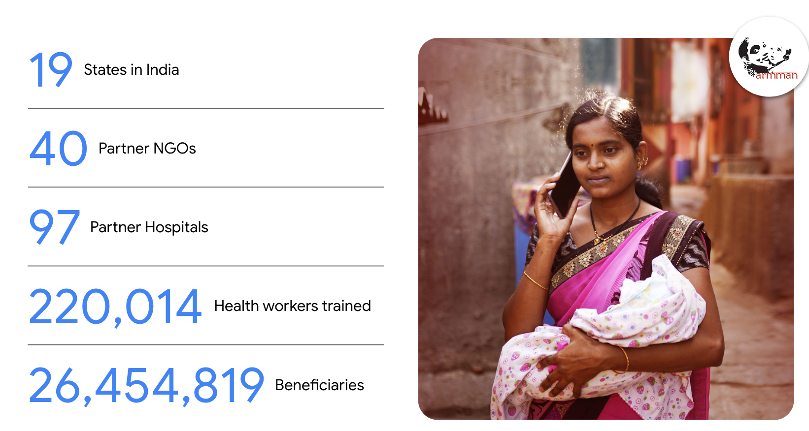
Overview of ARMMAN

One of the programs run by them is mMitra, which employs automated voice messaging to deliver timely preventive care information to expecting and new mothers during pregnancy and until one year after birth. These messages are tailored according to the gestational age of the beneficiary. Regular listenership to these messages has been shown to have a high correlation with improved behavioral and health outcomes, such as a 17% increase in infants with tripled birth weight at end of year and a 36% increase in women knowing the importance of taking iron tablets.

However, a key challenge ARMMAN faced was that about 40% of women gradually stopped engaging with the program. While it’s possible to mitigate this with live service calls to women to explain the advantage of listening to the messages, it is infeasible to call all the low listeners in the program because of limited support staff — this highlights the importance of effectively prioritizing who receives such service calls.

In “Field Study in Deploying Restless Multi-Armed Bandits: Assisting Non-Profits in Improving Maternal and Child Health”, published in AAAI 2022, we describe an ML-based solution that uses historical data from the NGO to predict which beneficiaries will benefit most from service calls. We address the challenges that come with a large-scale real world deployment of such a system and show the usefulness of deploying this model in a real study involving over 23,000 participants. The model showed an increase in listenership of 30% compared to the current standard of care group.

Background
We model this resource optimization problem using restless multi-armed bandits (RMABs), which have been well studied for application to such problems in a myriad of domains, including healthcare. An RMAB consists of n arms where each arm (representing a beneficiary) is associated with a two-state Markov decision process (MDP). Each MDP is modeled as a two-state (good or bad state, where the good state corresponds to high listenership in the previous week), two-action (corresponding to whether the beneficiary was chosen to receive a service call or not) problem. Further, each MDP has an associated reward function (i.e., the reward accumulated at a given state and action) and a transition function indicating the probability of moving from one state to the next under a given action, under the Markov condition that the next state depends only on the previous state and the action taken on that arm in that time step. The term restless indicates that all arms can change state irrespective of the action.
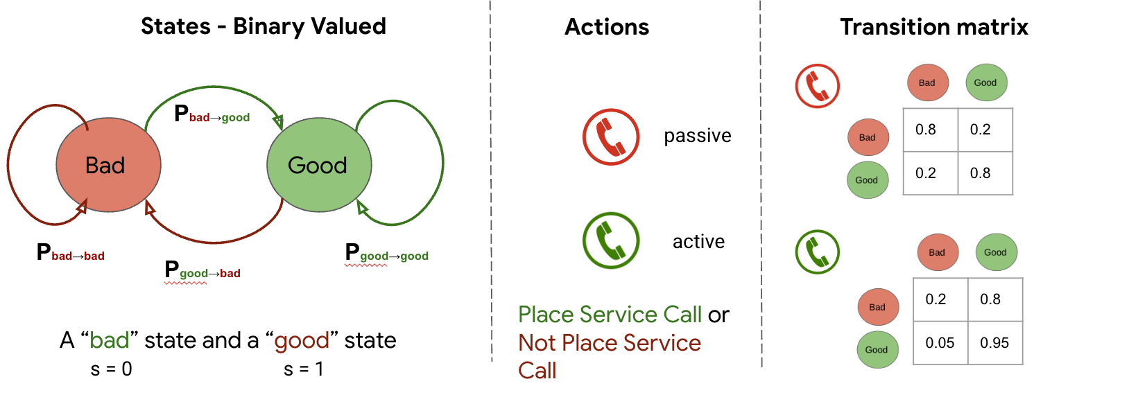
State of a beneficiary may transition from good (high engagement) to bad (low engagement) with example passive and active transition probabilities shown in the transition matrix.

Model Development
Finally, the RMAB problem is modeled such that at any time step, given n total arms, which k arms should be acted on (i.e., chosen to receive a service call), to maximize reward (engagement with the program).

The probability of transitioning from one state to another with (active probability) or without (passive probability) receiving a service call are therefore the underlying model parameters that are critical to solving the above optimization. To estimate these parameters, we use the demographic data of the beneficiaries collected at time of enrolment by the NGO, such as age, income, education, number of children, etc., as well as past listenership data, all in-line with the NGO’s data privacy standards (more below).

However, the limited volume of service calls limits the data corresponding to receiving a service call. To mitigate this, we use clustering techniques to learn from the collective observations of beneficiaries within a cluster and enable overcoming the challenge of limited samples per individual beneficiary.

In particular, we perform clustering on listenership behaviors, and then compute a mapping from the demographic features to each cluster.

Clustering on past listenership data reveals clusters with beneficiaries that behave similarly. We then infer a mapping from demographic features to clusters.

This mapping is useful because when a new beneficiary is enrolled, we only have access to their demographic information and have no knowledge of their listenership patterns, since they haven’t had a chance to listen yet. Using the mapping, we can infer transition probabilities for any new beneficiary that enrolls into the system.

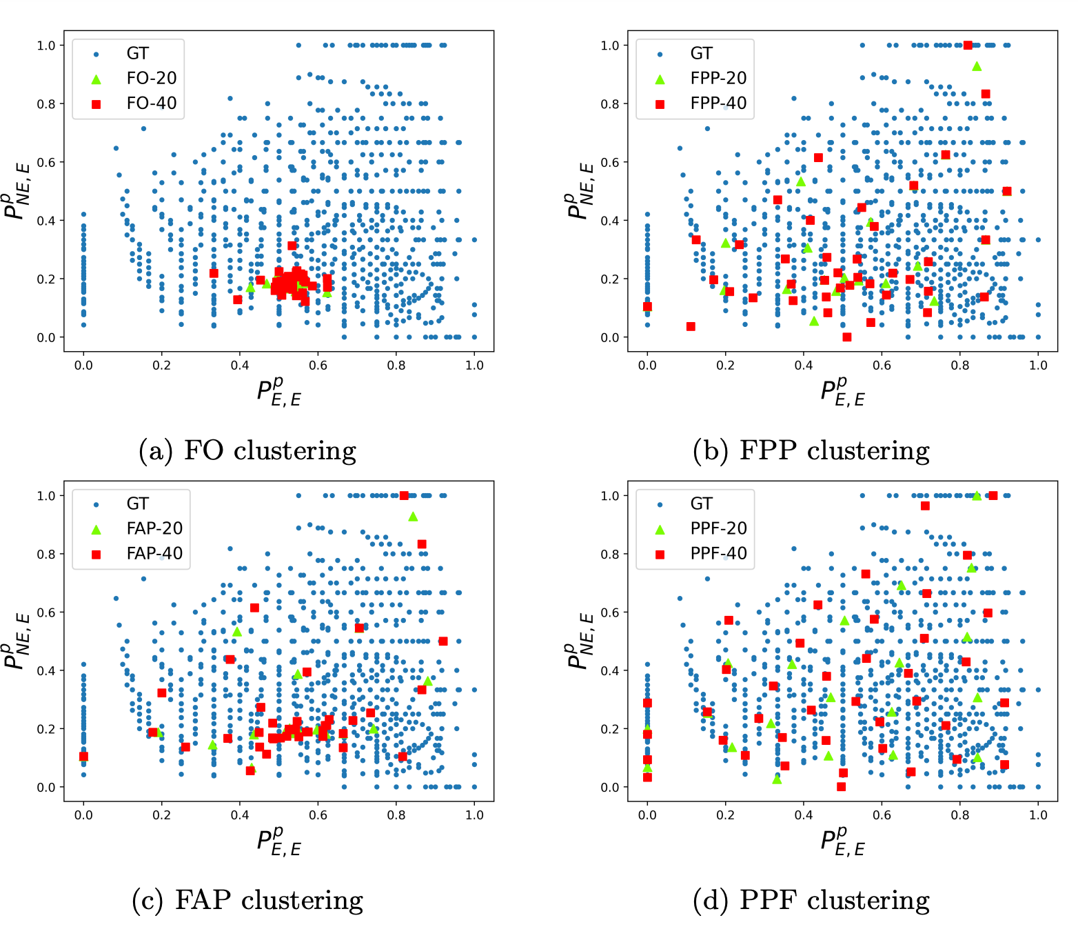
We used several qualitative and quantitative metrics to infer the optimal set of of clusters and explored different combinations of training data (demographic features only, features plus passive probabilities, features plus all probabilities, passive probabilities only) to achieve the most meaningful clusters, that are representative of the underlying data distribution and have a low variance in individual cluster sizes.

Comparison of passive transition probabilities obtained from different clustering methods with number of clusters s = 20 (red dots) and 40 (green dots), using ground truth passive transition probabilities (blue dots). Clustering based on features+passive probabilities (PPF) captures more distinct beneficiary behaviors across the probability space.

Clustering has the added advantage of reducing computational cost for resource-limited NGOs, as the optimization needs to be solved at a cluster level rather than an individual level. Finally, solving RMAB’s is known to be P-space hard, so we choose to solve the optimization using the popular Whittle index approach, which ultimately provides a ranking of beneficiaries based on their likely benefit of receiving a service call.

Results
We evaluated the model in a real world study consisting of approximately 23,000 beneficiaries who were divided into three groups: the current standard of care (CSOC) group, the "round robin" (RR) group, and the RMAB group. The beneficiaries in the CSOC group follow the original standard of care, where there are no NGO initiated service calls. The RR group represents the scenario where the NGO often conducts service calls using some systematic set order — the idea here is to have an easily executable policy that services enough of a cross-section of beneficiaries and can be scaled up or down per week based on available resources (this is the approach used by the NGO in this particular case, but the approach may vary for different NGOs). The RMAB group receives service calls as predicted by the RMAB model. All the beneficiaries across the three groups continue to receive the automated voice messages independent of the service calls.

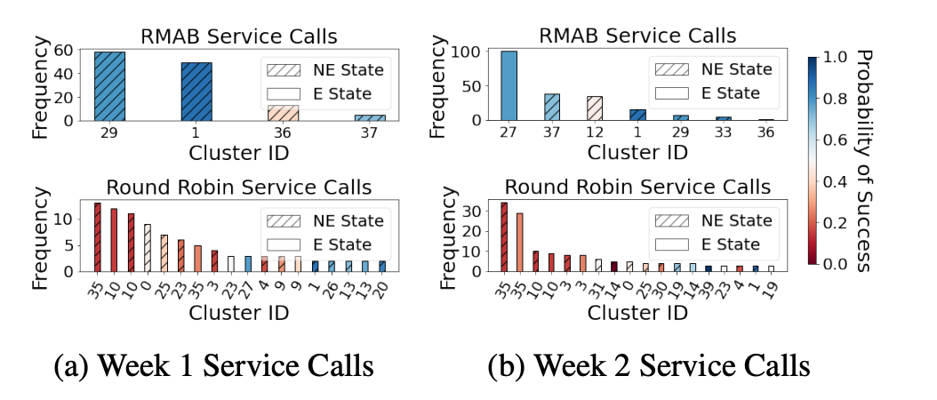
Distributions of clusters picked for service calls by RMAB and RR in week 1 (left) and 2 (right) are significantly different. RMAB is very strategic in picking only a few clusters with a promising probability of success (blue is high and red is low), RR displays no such strategic selection.

At the end of seven weeks, RMAB-based service calls resulted in the highest (and statistically significant) reduction in cumulative engagement drops (32%) compared to the CSOC group.

The plot shows cumulative engagement drops prevented compared to the control group.
   RMAB vs CSOC       RR vs CSOC       RMAB vs RR   
% reduction in cumulative engagement drops    32.0% 5.2% 28.3%
p-value 0.044 0.740 0.098

Ethical Considerations
An ethics board at the NGO reviewed the study. We took significant measures to ensure participant consent is understood and recorded in a language of the community's choice at each stage of the program. Data stewardship resides in the hands of the NGO, and only the NGO is allowed to share data. The code will soon be available publicly. The pipeline only uses anonymized data and no personally identifiable information (PII) is made available to the models. Sensitive data, such as caste, religion, etc., are not collected by ARMMAN for mMitra. Therefore, in pursuit of ensuring fairness of the model, we worked with public health and field experts to ensure other indicators of socioeconomic status were measured and adequately evaluated as shown below.
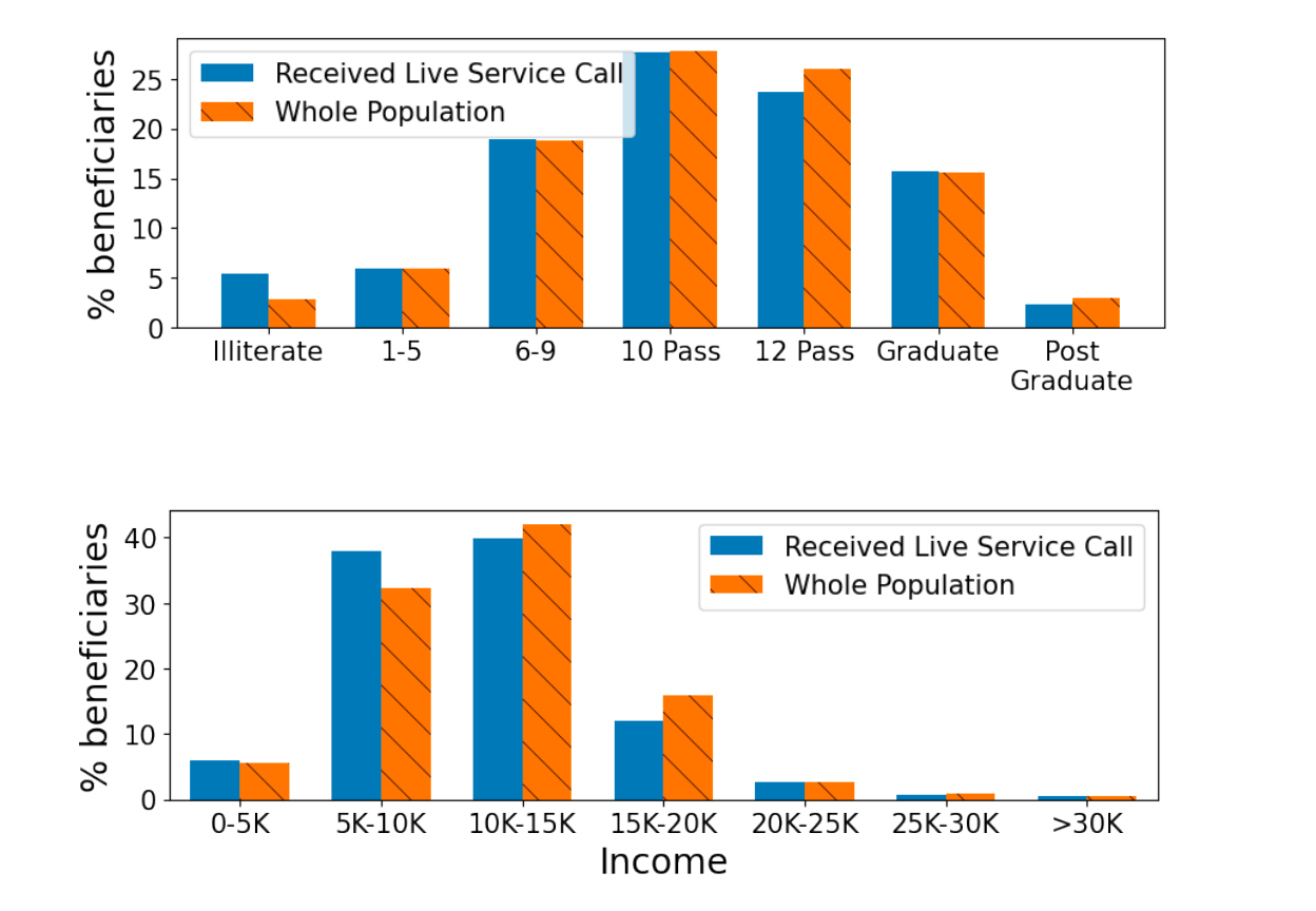
Distribution of highest education received (top) and monthly family income in Indian Rupees (bottom) across a cohort that received service calls compared to the whole population.

The proportion of beneficiaries that received a live service call within each income bracket reasonably matches the proportion in the overall population. However, differences are observed in lower income categories, where the RMAB model favors beneficiaries with lower income and beneficiaries with no formal education. Lastly, domain experts at ARMMAN have been deeply involved in the development and testing of this system and have provided continuous input and oversight in data interpretation, data consumption, and model design.

Conclusions
After thorough testing, the NGO has currently deployed this system for scheduling of service calls on a weekly basis. We are hopeful that this will pave the way for more deployments of ML algorithms for social impact in partnerships with non-profits in service of populations that have so far benefited less from ML. This work was also featured in Google for India 2021.

Acknowledgements
This work is part of our AI for Social Good efforts and was led by Google Research, India. Thanks to all our collaborators at ARMMAN, Google Research India, Google.org, and University Relations: Aparna Hegde, Neha Madhiwalla, Suresh Chaudhary, Aditya Mate, Lovish Madaan, Shresth Verma, Gargi Singh, Divy Thakkar.


1ARMMAN runs multiple programs to provide preventive care information to women through pregnancy and infancy enabling them to seek care, as well as programs to train and support health workers for timely detection and management of high-risk conditions. 

Source: Google AI Blog


Mapping Urban Trees Across North America with the Auto Arborist Dataset

Over four billion people live in cities around the globe, and while most people interact daily with others — at the grocery store, on public transit, at work — they may take for granted their frequent interactions with the diverse plants and animals that comprise fragile urban ecosystems. Trees in cities, called urban forests, provide critical benefits for public health and wellbeing and will prove integral to urban climate adaptation. They filter air and water, capture stormwater runoff, sequester atmospheric carbon dioxide, and limit erosion and drought. Shade from urban trees reduces energy-expensive cooling costs and mitigates urban heat islands. In the US alone, urban forests cover 127M acres and produce ecosystem services valued at $18 billion. But as the climate changes these ecosystems are increasingly under threat.

Census data is typically not comprehensive, covering a subset of public trees and not including those in parks.

Urban forest monitoring — measuring the size, health, and species distribution of trees in cities over time — allows researchers and policymakers to (1) quantify ecosystem services, including air quality improvement, carbon sequestration, and benefits to public health; (2) track damage from extreme weather events; and (3) target planting to improve robustness to climate change, disease and infestation.

However, many cities lack even basic data about the location and species of their trees. Collecting such data via a tree census is costly (a recent Los Angeles census cost $2 million and took 18 months) and thus is typically conducted only by cities with substantial resources. Further, lack of access to urban greenery is a key aspect of urban social inequality, including socioeconomic and racial inequality. Urban forest monitoring enables the quantification of this inequality and the pursuit of its improvement, a key aspect of the environmental justice movement. But machine learning could dramatically lower tree census costs using a combination of street-level and aerial imagery. Such an automated system could democratize access to urban forest monitoring, especially for under-resourced cities that are already disproportionately affected by climate change. While there have been prior efforts to develop automated urban tree species recognition from aerial or street-level imagery, a major limitation has been a lack of large-scale labeled datasets.

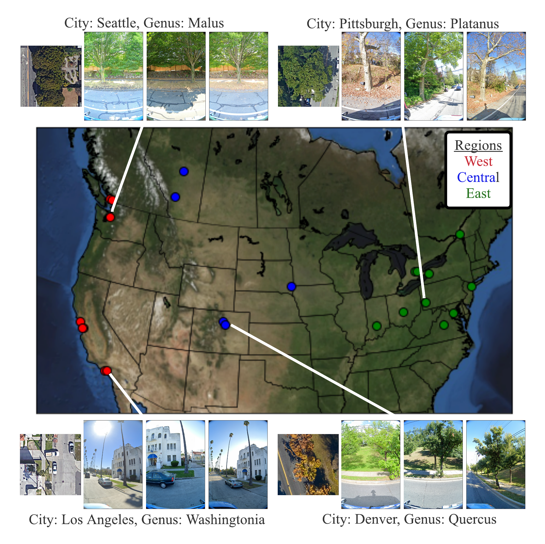
Today we introduce the Auto Arborist Dataset, a multiview urban tree classification dataset that, at ~2.6 million trees and >320 genera, is two orders of magnitude larger than those in prior work. To build the dataset, we pulled from public tree censuses from 23 North American cities (shown above) and merged these records with Street View and overhead RGB imagery. As the first urban forest dataset to cover multiple cities, we analyze in detail how forest models can generalize with respect to geographic distribution shifts, crucial to building systems that scale. We are releasing all 2.6M tree records publicly, along with aerial and ground-level imagery for 1M trees.

The 23 cities in the dataset are spread across North America, and are categorized into West, Central, and East regions to enable analysis of spatial and hierarchical generalization.
The number of tree records and genera in the dataset, per city and per region. The holdout city (which is never seen during training in any capacity) for each region is in bold.

The Auto Arborist Dataset
To curate Auto Arborist, we started from existing tree censuses which are provided by many cities online. For each tree census considered, we verified that the data contained GPS locations and genus/species labels, and was available for public use. We then parsed these data into a common format, fixing common data entry errors (such as flipped latitude/longitude) and mapping ground-truth genus names (and their common misspellings or alternate names) to a unified taxonomy. We have chosen to focus on genus prediction (instead of species-level prediction) as our primary task to avoid taxonomic complexity arising from hybrid and subspecies and the fact that there is more universal consensus on genus names than species names.

Next, using the provided geolocation for each tree, we queried an RGB aerial image centered on the tree and all street-level images taken within 2-10 meters around it. Finally, we filtered these images to (1) maximize our chances that the tree of interest is visible from each image and (2) preserve user privacy. This latter concern involved a number of steps including the removal of images that included people as determined by semantic segmentation and manual blurring, among others.

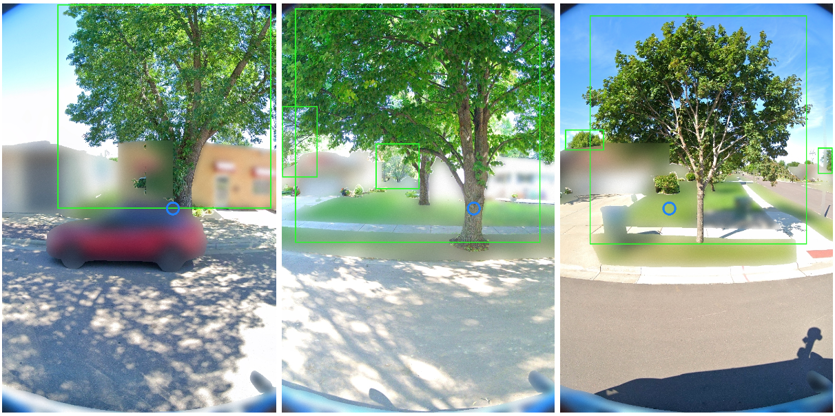
Selected Street View imagery from the Auto Arborist dataset. Green boxes represent tree detections (using a model trained on Open Images) and blue dots represent projected GPS location of the labeled tree.

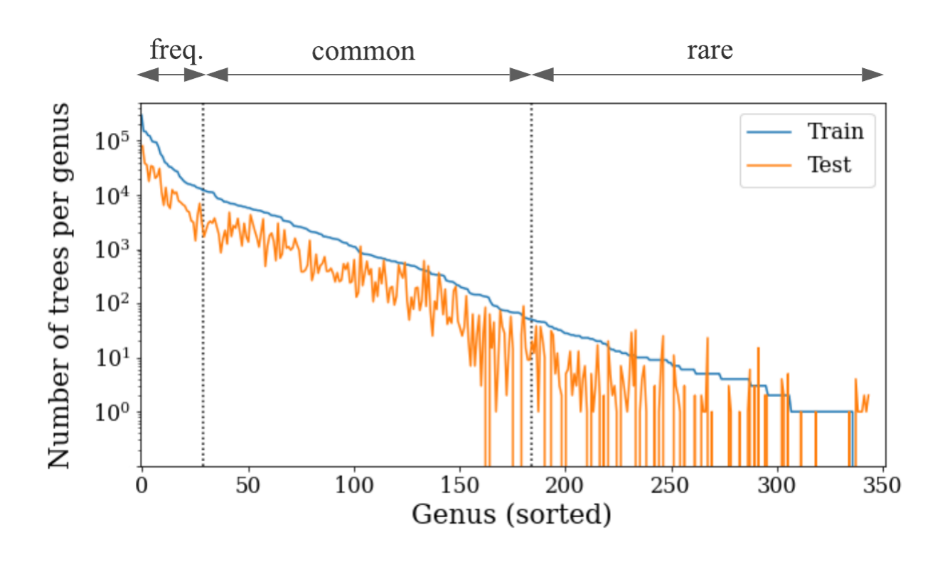
One of the most important challenges for urban forest monitoring is to do well in cities that were not part of the training set. Vision models must contend with distribution shifts, where the training distribution differs from the test distribution from a new city. Genus distributions vary geographically (e.g., there are more Douglas fir in western Canada than in California) and can also vary based on city size (LA is much larger than Santa Monica and contains many more genera). Another challenge is the long-tailed, fine-grained nature of tree genera, which can be difficult to disambiguate even for human experts, with many genera being quite rare.

The long-tailed distribution across Auto Arborist categories. Most examples come from a few frequent categories, and many categories have far fewer examples. We characterize each genus as frequent, common, or rare based on the number of training examples. Note that the test data is split spatially from the training data within each city, so not all rare genera are seen in the test set.

Finally, there are a number of ways in which tree images can have noise. For one, there is temporal variation in deciduous trees (for example, when aerial imagery includes leaves, but street-level images are bare). Moreover, public arboreal censuses are not always up-to-date. Thus, sometimes trees have died (and are no longer visible) in the time since the tree census was taken. In addition, aerial data quality can be poor (missing or obscured, e.g., by clouds).

Our curation process sought to minimize these issues by (1) only keeping images with sufficient tree pixels, as determined by a semantic segmentation model, (2) only keeping reasonably recent images, and (3) only keeping images where the tree position was sufficiently close to the street level camera. We considered also optimizing for trees seen in spring and summer, but decided seasonal variation could be a useful cue — we thus also released the date of each image to enable the community to explore the effects of seasonal variability.

Benchmark and Evaluation
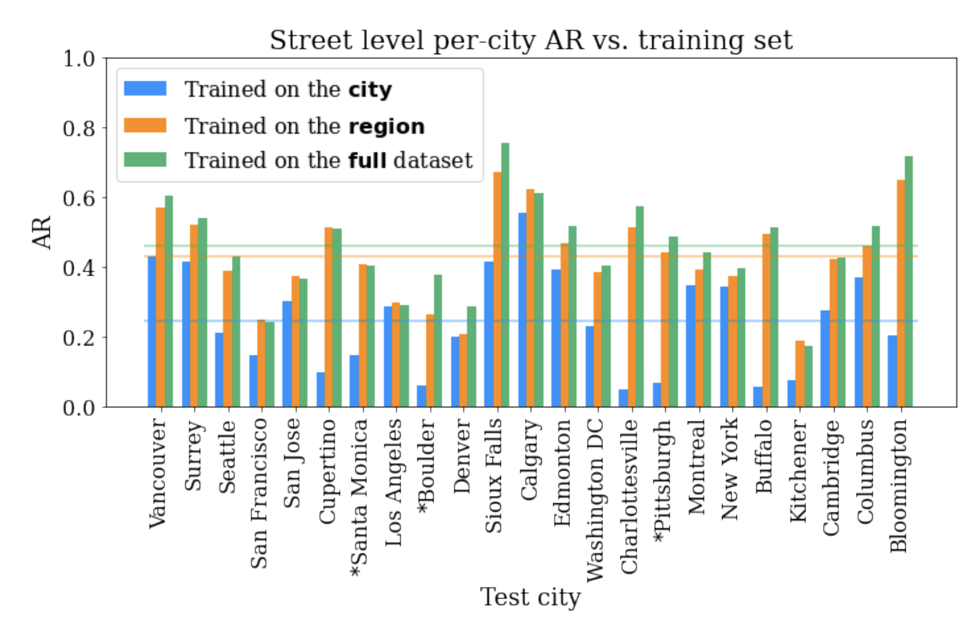
To evaluate the dataset, we designed a benchmark to measure domain generalization and performance in the long tail of the distribution. We generated training and test splits at three levels. First, we split within each city (based on latitude or longitude) to see how well a city generalizes to itself. Second, we aggregate city-level training sets into three regions, West, Central, and East, holding out one city from each region. Finally, we merge the training sets across the three regions. For each of these splits, we report both accuracy and class-averaged recall for frequent, common and rare species on the corresponding held-out test sets.

Using these metrics, we establish a performance baseline using standard modern convolutional models (ResNet). Our results demonstrate the benefits of a large-scale, geospatially distributed dataset such as Auto Arborist. First, we see that more training data helps — training on the entire dataset is better than training on a region, which is better than training on a single city.

The performance on each city’s test set when training on itself, on the region, and on the full training set.

Second, training on similar cities helps (and thus, having more coverage of cities helps). For example, if focusing on Seattle, then it is better to train on trees in Vancouver than Pittsburgh.

Cross-set performance, looking at the pairwise combination of train and test sets for each city. Note the block-diagonal structure, which highlights regional structure in the dataset.

Third, more data modalities and views help. The best performing models combine inputs from multiple Street View angles and overhead views. There remains much room for improvement, however, and this is where we believe the larger community of researchers can help.

Get Involved
By releasing the Auto Arborist Dataset, we step closer to the goal of affordable urban forest monitoring, enabling the computer vision community to tackle urban forest monitoring at scale for the first time. In the future, we hope to expand coverage to more North American cities (particularly in the South of the US and Mexico) and even worldwide. Further, we are excited to push the dataset to the more fine-grained species level and investigate more nuanced monitoring, including monitoring tree health and growth over time, and studying the effects of environmental factors on urban forests.

For more details, see our CVPR 2022 paper. This dataset is part of Google's broader efforts to empower cities with data about urban forests, through the Environmental Insights Explorer Tree Canopy Lab and is available on our GitHub repo. If you represent a city that is interested in being included in the dataset please email [email protected].

Acknowledgements
We would like to thank our co-authors Guanhang Wu, Trevor Edwards, Filip Pavetic, Bo Majewski, Shreyasee Mukherjee, Stanley Chan, John Morgan, Vivek Rathod, and Chris Bauer. We also thank Ruth Alcantara, Tanya Birch, and Dan Morris from Google AI for Nature and Society, John Quintero, Stafford Marquardt, Xiaoqi Yin, Puneet Lall, and Matt Manolides from Google Geo, Karan Gill, Tom Duerig, Abhijit Kundu, David Ross, Vighnesh Birodkar from Google Research (Perception team), and Pietro Perona for their support. This work was supported in part by the Resnick Sustainability Institute and was undertaken while Sara Beery was a Student Researcher at Google.

Source: Google AI Blog


Unlocking Zero-Resource Machine Translation to Support New Languages in Google Translate

Machine translation (MT) technology has made significant advances in recent years, as deep learning has been integrated with natural language processing (NLP). Performance on research benchmarks like WMT have soared, and translation services have improved in quality and expanded to include new languages. Nevertheless, while existing translation services cover languages spoken by the majority of people world wide, they only include around 100 languages in total, just over 1% of those actively spoken globally. Moreover, the languages that are currently represented are overwhelmingly European, largely overlooking regions of high linguistic diversity, like Africa and the Americas.

There are two key bottlenecks towards building functioning translation models for the long tail of languages. The first arises from data scarcity; digitized data for many languages is limited and can be difficult to find on the web due to quality issues with Language Identification (LangID) models. The second challenge arises from modeling limitations. MT models usually train on large amounts of parallel (translated) text, but without such data, models must learn to translate from limited amounts of monolingual text, which is a novel area of research. Both of these challenges need to be addressed for translation models to reach sufficient quality.

In “Building Machine Translation Systems for the Next Thousand Languages”, we describe how to build high-quality monolingual datasets for over a thousand languages that do not have translation datasets available and demonstrate how one can use monolingual data alone to train MT models. As part of this effort, we are expanding Google Translate to include 24 under-resourced languages. For these languages, we created monolingual datasets by developing and using specialized neural language identification models combined with novel filtering approaches. The techniques we introduce supplement massively multilingual models with a self supervised task to enable zero-resource translation. Finally, we highlight how native speakers have helped us realize this accomplishment.

Meet the Data
Automatically gathering usable textual data for under-resourced languages is much more difficult than it may seem. Tasks like LangID, which work well for high-resource languages, are unsuccessful for under-resourced languages, and many publicly available datasets crawled from the web often contain more noise than usable data for the languages they attempt to support. In our early attempts to identify under-resourced languages on the web by training a standard Compact Language Detector v3 (CLD3) LangID model, we too found that the dataset was too noisy to be usable.

As an alternative, we trained a Transformer-based, semi-supervised LangID model on over 1000 languages. This model supplements the LangID task with the MAsked Sequence-to-Sequence (MASS) task to better generalize over noisy web data. MASS simply garbles the input by randomly removing sequences of tokens from it, and trains the model to predict these sequences. We applied the Transformer-based model to a dataset that had been filtered with a CLD3 model and trained to recognize clusters of similar languages.

We then applied the open sourced Term Frequency-Inverse Internet Frequency (TF-IIF) filtering to the resulting dataset to find and discard sentences that were actually in related high-resource languages, and developed a variety of language-specific filters to eliminate specific pathologies. The result of this effort was a dataset with monolingual text in over 1000 languages, of which 400 had over 100,000 sentences. We performed human evaluations on samples of 68 of these languages and found that the majority (>70%) reflected high-quality, in-language content.

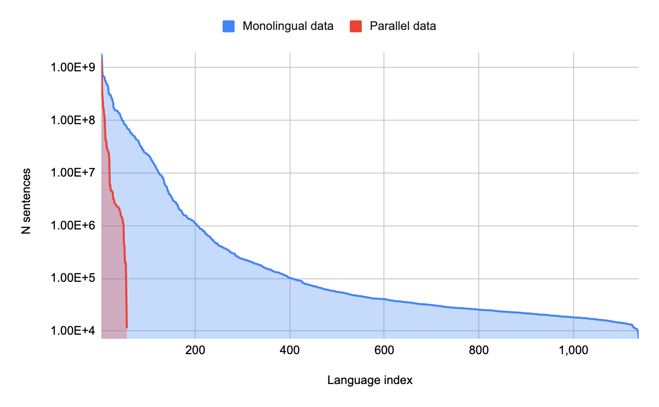
The amount of monolingual data per language versus the amount of parallel (translated) data per language. A small number of languages have large amounts of parallel data, but there is a long tail of languages with only monolingual data.

Meet the Models
Once we had a dataset of monolingual text in over 1000 languages, we then developed a simple yet practical approach for zero-resource translation, i.e., translation for languages with no in-language parallel text and no language-specific translation examples. Rather than limiting our model to an artificial scenario with only monolingual text, we also include all available parallel text data with millions of examples for higher resource languages to enable the model to learn the translation task. Simultaneously, we train the model to learn representations of under-resourced languages directly from monolingual text using the MASS task. In order to solve this task, the model is forced to develop a sophisticated representation of the language in question, developing a complex understanding of how words relate to other words in a sentence.

Relying on the benefits of transfer learning in massively multilingual models, we train a single giant translation model on all available data for over 1000 languages. The model trains on monolingual text for all 1138 languages and on parallel text for a subset of 112 of the higher-resourced languages.

At training time, any input the model sees has a special token indicating which language the output should be in, exactly like the standard formulation for multilingual translation. Our additional innovation is to use the same special tokens for both the monolingual MASS task and the translation task. Therefore, the token translate_to_french may indicate that the source is in English and needs to be translated to French (the translation task), or it may mean that the source is in garbled French and needs to be translated to fluent French (the MASS task). By using the same tags for both tasks, a translate_to_french tag takes on the meaning, “Produce a fluent output in French that is semantically close to the input, regardless of whether the input is garbled in the same language or in another language entirely. From the model’s perspective, there is not much difference between the two.

Surprisingly, this simple procedure produces high quality zero-shot translations. The BLEU and ChrF scores for the resulting model are in the 10–40 and 20–60 ranges respectively, indicating mid- to high-quality translation. We observed meaningful translations even for highly inflected languages like Quechua and Kalaallisut, despite these languages being linguistically dissimilar to all other languages in the model. However, we only computed these metrics on the small subset of languages with human-translated evaluation sets. In order to understand the quality of translation for the remaining languages, we developed an evaluation metric based on round-trip translation, which allowed us to see that several hundred languages are reaching high translation quality.

To further improve quality, we use the model to generate large amounts of synthetic parallel data, filter the data based on round-trip translation (comparing a sentence translated into another language and back again), and continue training the model on this filtered synthetic data via back-translation and self-training. Finally, we fine-tune the model on a smaller subset of 30 languages and distill it into a model small enough to be served.

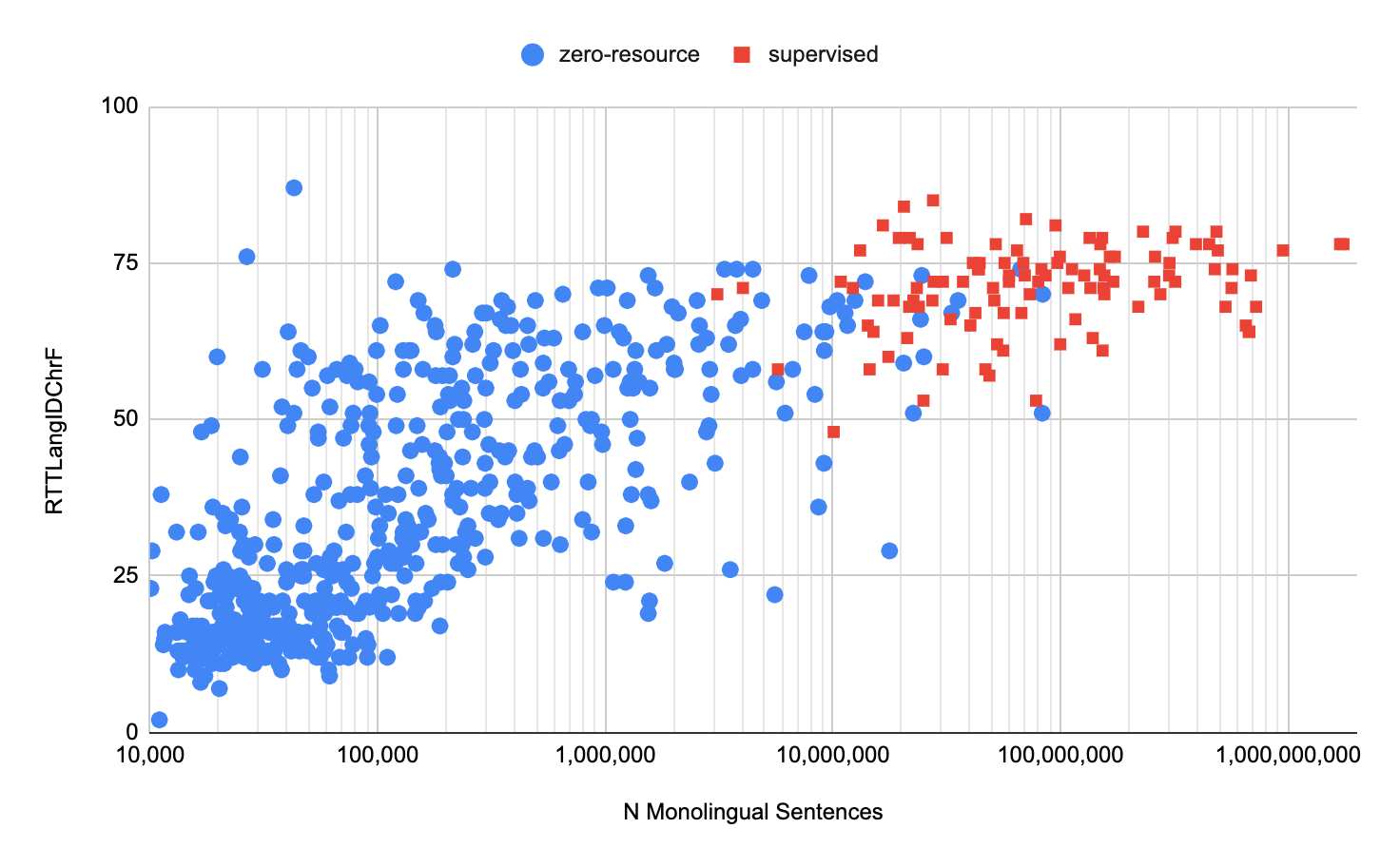
Translation accuracy scores for 638 of the languages supported in our model, using the metric we developed (RTTLangIDChrF), for both the higher-resource supervised languages and the low-resource zero-resource languages.

Contributions from Native Speakers
Regular communication with native speakers of these languages was critical for our research. We collaborated with over 100 people at Google and other institutions who spoke these languages. Some volunteers helped develop specialized filters to remove out-of-language content overlooked by automatic methods, for instance Hindi mixed with Sanskrit. Others helped with transliterating between different scripts used by the languages, for instance between Meetei Mayek and Bengali, for which sufficient tools didn’t exist; and yet others helped with a gamut of tasks related to evaluation. Native speakers were also key for advising in matters of political sensitivity, like the appropriate name for the language, and the appropriate writing system to use for it. And only native speakers could answer the ultimate question: given the current quality of translation, would it be valuable to the community for Google Translate to support this language?

Closing Notes
This advance is an exciting first step toward supporting more language technologies in under-resourced languages. Most importantly, we want to stress that the quality of translations produced by these models still lags far behind that of the higher-resource languages supported by Google Translate. These models are certainly a useful first tool for understanding content in under-resourced languages, but they will make mistakes and exhibit their own biases. As with any ML-driven tool, one should consider the output carefully.

The complete list of new languages added to Google Translate in this update:

Acknowledgements
We would like to thank Julia Kreutzer, Orhan Firat, Daan van Esch, Aditya Siddhant, Mengmeng Niu, Pallavi Baljekar, Xavier Garcia, Wolfgang Macherey, Theresa Breiner, Vera Axelrod, Jason Riesa, Yuan Cao, Mia Xu Chen, Klaus Macherey, Maxim Krikun, Pidong Wang, Alexander Gutkin, Apurva Shah, Yanping Huang, Zhifeng Chen, Yonghui Wu, and Macduff Hughes for their contributions to the research, engineering, and leadership of this project.

We would also like to extend our deepest gratitude to the following native speakers and members of affected communities, who helped us in a wide variety of ways: Yasser Salah Eddine Bouchareb (Algerian Arabic); Mfoniso Ukwak (Anaang); Bhaskar Borthakur, Kishor Barman, Rasika Saikia, Suraj Bharech (Assamese); Ruben Hilare Quispe (Aymara); Devina Suyanto (Balinese); Allahserix Auguste Tapo, Bakary Diarrassouba, Maimouna Siby (Bambara); Mohammad Jahangir (Baluchi); Subhajit Naskar (Bengali); Animesh Pathak, Ankur Bapna, Anup Mohan, Chaitanya Joshi, Chandan Dubey, Kapil Kumar, Manish Katiyar, Mayank Srivastava, Neeharika, Saumya Pathak, Tanya Sinha, Vikas Singh (Bhojpuri); Bowen Liang, Ellie Chio, Eric Dong, Frank Tang, Jeff Pitman, John Wong, Kenneth Chang, Manish Goregaokar, Mingfei Lau, Ryan Li, Yiwen Luo (Cantonese); Monang Setyawan (Caribbean Javanese); Craig Cornelius (Cherokee); Anton Prokopyev (Chuvash); Rajat Dogra, Sid Dogra (Dogri); Mohamed Kamagate (Dyula); Chris Assigbe, Dan Ameme, Emeafa Doe, Irene Nyavor, Thierry Gnanih, Yvonne Dumor (Ewe); Abdoulaye Barry, Adama Diallo, Fauzia van der Leeuw, Ibrahima Barry (Fulfulde); Isabel Papadimitriou (Greek); Alex Rudnick (Guarani); Mohammad Khdeir (Gulf Arabic); Paul Remollata (Hiligaynon); Ankur Bapna (Hindi); Mfoniso Ukwak (Ibibio); Nze Lawson (Igbo); D.J. Abuy, Miami Cabansay (Ilocano); Archana Koul, Shashwat Razdan, Sujeet Akula (Kashmiri); Jatin Kulkarni, Salil Rajadhyaksha, Sanjeet Hegde Desai, Sharayu Shenoy, Shashank Shanbhag, Shashi Shenoy (Konkani); Ryan Michael, Terrence Taylor (Krio); Bokan Jaff, Medya Ghazizadeh, Roshna Omer Abdulrahman, Saman Vaisipour, Sarchia Khursheed (Kurdish (Sorani));Suphian Tweel (Libyan Arabic); Doudou Kisabaka (Lingala); Colleen Mallahan, John Quinn (Luganda); Cynthia Mboli (Luyia); Abhishek Kumar, Neeraj Mishra, Priyaranjan Jha, Saket Kumar, Snehal Bhilare (Maithili); Lisa Wang (Mandarin Chinese); Cibu Johny (Malayalam); Viresh Ratnakar (Marathi); Abhi Sanoujam, Gautam Thockchom, Pritam Pebam, Sam Chaomai, Shangkar Mayanglambam, Thangjam Hindustani Devi (Meiteilon (Manipuri)); Hala Ajil (Mesopotamian Arabic); Hamdanil Rasyid (Minangkabau); Elizabeth John, Remi Ralte, S Lallienkawl Gangte,Vaiphei Thatsing, Vanlalzami Vanlalzami (Mizo); George Ouais (MSA); Ahmed Kachkach, Hanaa El Azizi (Morrocan Arabic); Ujjwal Rajbhandari (Newari); Ebuka Ufere, Gabriel Fynecontry, Onome Ofoman, Titi Akinsanmi (Nigerian Pidgin); Marwa Khost Jarkas (North Levantine Arabic); Abduselam Shaltu, Ace Patterson, Adel Kassem, Mo Ali, Yonas Hambissa (Oromo); Helvia Taina, Marisol Necochea (Quechua); AbdelKarim Mardini (Saidi Arabic); Ishank Saxena, Manasa Harish, Manish Godara, Mayank Agrawal, Nitin Kashyap, Ranjani Padmanabhan, Ruchi Lohani, Shilpa Jindal, Shreevatsa Rajagopalan, Vaibhav Agarwal, Vinod Krishnan (Sanskrit); Nabil Shahid (Saraiki); Ayanda Mnyakeni (Sesotho, Sepedi); Landis Baker (Seychellois Creole); Taps Matangira (Shona); Ashraf Elsharif (Sudanese Arabic); Sakhile Dlamini (Swati); Hakim Sidahmed (Tamazight); Melvin Johnson (Tamil); Sneha Kudugunta (Telugu); Alexander Tekle, Bserat Ghebremicael, Nami Russom, Naud Ghebre (Tigrinya); Abigail Annkah, Diana Akron, Maame Ofori, Monica Opoku-Geren, Seth Duodu-baah, Yvonne Dumor (Twi); Ousmane Loum (Wolof); and Daniel Virtheim (Yiddish).


Source: Google AI Blog


Predicting Text Readability from Scrolling Interactions

Illiteracy affects at least 773 million people globally, both young and old. For these individuals, reading information from unfamiliar sources or on unfamiliar topics can be extremely difficult. Unfortunately, these inequalities have been further magnified by the global pandemic as a result of unequal access to education in reading and writing. In fact, UNESCO reports that over 100 million children are falling behind the minimum proficiency level in reading due to COVID-related school closures.

With increasing world-wide access to technology, reading on a device, such as a tablet or phone, has largely taken the place of traditional formats. This provides a unique opportunity to observe reading interactions, e.g., how a reader scrolls through a text, which can inform our understanding of what can make text difficult to read. This understanding is crucial when designing educational applications for low-proficiency readers and language learners, because it can be used to match learners with appropriately leveled texts as well as to support readers in understanding texts beyond their reading level.

In “Predicting Text Readability from Scrolling Interactions”, presented at CoNLL 2021, we show that data from on-device reading interactions can be used to predict how readable a text is. This novel approach provides insights into subjective readability — whether an individual reader has found a text accessible — and demonstrates that existing readability models can be improved by including feedback from scroll-based reading interactions. In order to encourage research in this area and to help enable more personalized tools for language learning and text simplification, we are releasing the dataset of reading interactions generated from our scrolling behavior–based readability assessment of English-language texts.

Understanding Text Difficulty
There are multiple aspects of a text that impact how difficult it is to read, including the vocabulary level, the syntactic structure, and overall coherence. Traditional machine learning approaches to measure readability have exclusively relied on such linguistic features. However, using these features alone does not work well for online content, because such content often contains abbreviations, emojis, broken text, and short passages, which detrimentally impact the performance of readability models.

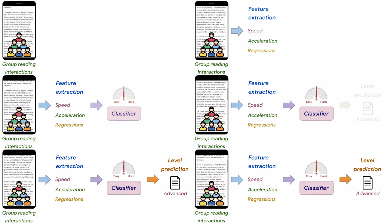
To address this, we investigated whether aggregate data about the reading interactions of a group can be used to predict how difficult a text is, as well as how reading interactions may differ based on a readers’ understanding. When reading on a device, readers typically interact with text by scrolling in a vertical fashion, which we hypothesize can be used as a coarse proxy for reading comprehension. With this in mind, we recruited 518 paid participants and asked them to read English-language texts of different difficulty levels. We recorded the reading interactions by measuring different features of the participants’ scrolling behavior, such as the speed, acceleration and number of times areas of text were revisited. We then used this information to produce a set of features for a readability classifier.

Predicting Text Difficulty from Scrolling Behavior
We investigated which types of scrolling behaviors were most impacted by text difficulty and tested the significance using linear mixed effect models. In our set up, we have repeated measures, as multiple participants read the same texts and each participant reads more than one text. Using linear mixed-effect models gives us a higher confidence that the differences in interactions we are observing are because of the text difficulty, and not other random effects.

Our results showed that multiple reading behaviors differed significantly based on the text level, for example, the average, maximum and minimum acceleration of scrolling. We found the most significant features to be the total read time and the maximum reading speeds.

We then used these features as inputs to a machine learning algorithm. We designed and trained a support vector machine (i.e., a binary classifier) to predict whether a text is either advanced or elementary based only on scrolling behaviors as individuals interacted with it. The dataset on which the model was trained contains 60 articles, each of which were read by an average of 17 participants. From these interactions we produced aggregate features by taking the mean of the significant measures across participants.


We measured the accuracy of the approach using a metric called f-score, which measures how accurate the model is at classifying a text as either “easy” or “difficult” (where 1.0 reflects perfect classification accuracy). We are able to achieve an f-score of 0.77 on this task, using interaction features alone. This is the first work to show that it is possible to predict the readability of a text using only interaction features.

Improving Readability Models
In order to demonstrate the value of applying readability measures from scrolling behaviors to existing readability models, we integrated scroll-based features into the state-of-the-art automated readability assessment tool, which was released as part of the OneStopEnglish corpus. We found that the addition of interaction features improves the f-score of this model from 0.84 to 0.88. In addition, we were able to significantly outperform this system by using interaction information with simple vocabulary features, such as the number of words in the text, achieving an impressive f-score of 0.96.

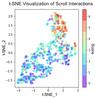
In our study, we recorded comprehension scores to evaluate the understanding and readability of text for individuals. Participants were asked three questions per article to assess the reader’s understanding of what they had read. The interaction features of an individual’s scrolling behavior was represented as a high dimensional vector. To explore this data, we visualized the reading interaction features for each participant using t-distributed stochastic neighbor embeddings, which is a statistical method for visualizing high-dimensional data. The results revealed clusters in the comprehension score based on how well individuals understood the text. This shows that there is implicit information in reading interactions about the likelihood that an individual has understood a given text. We refer to this phenomenon as subjective readability. This information can be very useful for educational applications or for simplifying online content.

Plot showing t-SNE projection of scroll interactions in 2-dimensions. The color of each data point corresponds to the comprehension score. Clusters of comprehension scores indicate that there are correlations between reading behaviors and comprehension.

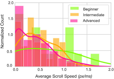
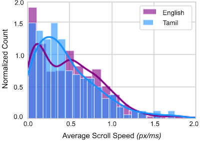
Finally, we investigated the extent to which reading interactions vary across audiences. We compared the average scrolling speed across different reader groups, covering reading proficiency and the reader’s first language. We found that the speed distribution varies depending on the proficiency and first language of the audience. This supports the case that first language and proficiency alter the reading behaviors of audiences, which allows us to contextualize the reading behavior of groups and better understand which areas of text may be harder for them to read.

Histogram showing the average speeds of scrolling (in vertical pixels per millisecond) across readers of different proficiency levels (beginner, intermediate and advanced), with lines showing the smoothed trend for each group. A higher average scroll speed indicates faster reading times. For example, a more challenging text that corresponds to slower scroll speeds by advanced readers is associated with higher scroll speeds by beginners because they engage with the text only superficially.

Histogram showing the average speeds of scrolling (in vertical pixels per millisecond) across audiences by first language of the readers, Tamil or English, with lines showing the smoothed trend for each group. A higher average scroll speed indicates faster reading times. Dark blue bars are where the histograms overlap.

Conclusion
This work is the first to show that reading interactions, such as scrolling behavior, can be used to predict the readability of text, which can yield numerous benefits. Such measures are language agnostic, unobtrusive, and robust to noisy text. Implicit user feedback allows insight into readability at an individual level, thereby allowing for a more inclusive and personalisable assessment of text difficulty. Furthermore, being able to judge the subjective readability of text benefits language learning and educational apps. We conducted a 518 participant study to investigate the impact of text readability on reading interactions and are releasing a novel dataset of the associated reading interactions. We confirm that there are statistically significant differences in the way that readers interact with advanced and elementary texts, and that the comprehension scores of individuals correlate with specific measures of scrolling interaction. For more information our conference presentation is available to view.

Acknowledgements
We thank our collaborators Yevgeni Berzak, Tony Mak and Matt Sharifi, as well as Dmitry Lagun and Blaise Aguera y Arcas for their helpful feedback on the paper.

Source: Google AI Blog


MetNet-2: Deep Learning for 12-Hour Precipitation Forecasting

Deep learning has successfully been applied to a wide range of important challenges, such as cancer prevention and increasing accessibility. The application of deep learning models to weather forecasts can be relevant to people on a day-to-day basis, from helping people plan their day to managing food production, transportation systems, or the energy grid. Weather forecasts typically rely on traditional physics-based techniques powered by the world’s largest supercomputers. Such methods are constrained by high computational requirements and are sensitive to approximations of the physical laws on which they are based.

Deep learning offers a new approach to computing forecasts. Rather than incorporating explicit physical laws, deep learning models learn to predict weather patterns directly from observed data and are able to compute predictions faster than physics-based techniques. These approaches also have the potential to increase the frequency, scope, and accuracy of the predicted forecasts.

Illustration of the computation through MetNet-2. As the computation progresses, the network processes an ever larger context from the input and makes a probabilistic forecast of the likely future weather conditions.

Within weather forecasting, deep learning techniques have shown particular promise for nowcasting — i.e., predicting weather up to 2-6 hours ahead. Previous work has focused on using direct neural network models for weather data, extending neural forecasts from 0 to 8 hours with the MetNet architecture, generating continuations of radar data for up to 90 minutes ahead, and interpreting the weather information learned by these neural networks. Still, there is an opportunity for deep learning to extend improvements to longer-range forecasts.

To that end, in “Skillful Twelve Hour Precipitation Forecasts Using Large Context Neural Networks”, we push the forecasting boundaries of our neural precipitation model to 12 hour predictions while keeping a spatial resolution of 1 km and a time resolution of 2 minutes. By quadrupling the input context, adopting a richer weather input state, and extending the architecture to capture longer-range spatial dependencies, MetNet-2 substantially improves on the performance of its predecessor, MetNet. Compared to physics-based models, MetNet-2 outperforms the state-of-the-art HREF ensemble model for weather forecasts up to 12 hours ahead.

MetNet-2 Features and Architecture
Neural weather models like MetNet-2 map observations of the Earth to the probability of weather events, such as the likelihood of rain over a city in the afternoon, of wind gusts reaching 20 knots, or of a sunny day ahead. End-to-end deep learning has the potential to both streamline and increase quality by directly connecting a system's inputs and outputs. With this in mind, MetNet-2 aims to minimize both the complexity and the total number of steps involved in creating a forecast.

The inputs to MetNet-2 include the radar and satellite images also used in MetNet. To capture a more comprehensive snapshot of the atmosphere with information such as temperature, humidity, and wind direction — critical for longer forecasts of up to 12 hours — MetNet-2 also uses the pre-processed starting state used in physical models as a proxy for this additional weather information. The radar-based measures of precipitation (MRMS) serve as the ground truth (i.e., what we are trying to predict) that we use in training to optimize MetNet-2’s parameters.

Example ground truth image: Instantaneous precipitation (mm/hr) based on radar (MRMS) capturing a 12 hours-long progression.

MetNet-2’s probabilistic forecasts can be viewed as averaging all possible future weather conditions weighted by how likely they are. Due to its probabilistic nature, MetNet-2 can be likened to physics-based ensemble models, which average some number of future weather conditions predicted by a variety of physics-based models. One notable difference between these two approaches is the duration of the core part of the computation: ensemble models take ~1 hour, whereas MetNet-2 takes ~1 second.

Steps in a MetNet-2 forecast and in a physics-based ensemble.

One of the main challenges that MetNet-2 must overcome to make 12 hour long forecasts is capturing a sufficient amount of spatial context in the input images. For each additional forecast hour we include 64 km of context in every direction at the input. This results in an input context of size 20482 km2 — four times that used in MetNet. In order to process such a large context, MetNet-2 employs model parallelism whereby the model is distributed across 128 cores of a Cloud TPU v3-128. Due to the size of the input context, MetNet-2 replaces the attentional layers of MetNet with computationally more efficient convolutional layers. But standard convolutional layers have local receptive fields that may fail to capture large spatial contexts, so MetNet-2 uses dilated receptive fields, whose size doubles layer after layer, in order to connect points in the input that are far apart one from the other.

Example of input spatial context and target area for MetNet-2.

Results
Because MetNet-2’s predictions are probabilistic, the model’s output is naturally compared with the output of similarly probabilistic ensemble or post-processing models. HREF is one such state-of-the-art ensemble model for precipitation in the United States, which aggregates ten predictions from five different models, twice a day. We evaluate the forecasts using established metrics, such as the Continuous Ranked Probability Score, which captures the magnitude of the probabilistic error of a model’s forecasts relative to the ground truth observations. Despite not performing any physics-based calculations, MetNet-2 is able to outperform HREF up to 12 hours into the future for both low and high levels of precipitation.

Continuous Ranked Probability Score (CRPS; lower is better) for MetNet-2 vs HREF aggregated over a large number of test patches randomly located in the Continental United States.

Examples of Forecasts
The following figures provide a selection of forecasts from MetNet-2 compared with the physics-based ensemble HREF and the ground truth MRMS.

Probability maps for the cumulative precipitation rate of 1 mm/hr on January 3, 2019 over the Pacific NorthWest. The maps are shown for each hour of lead time from 1 to 12. Left: Ground truth, source MRMS. Center: Probability map as predicted by MetNet-2 . Right: Probability map as predicted by HREF.
Comparison of 0.2 mm/hr precipitation on March 30, 2020 over Denver, Colorado. Left: Ground truth, source MRMS. Center: Probability map as predicted by MetNet-2 . Right: Probability map as predicted by HREF.MetNet-2 is able to predict the onset of the storm (called convective initiation) earlier in the forecast than HREF as well as the storm’s starting location, whereas HREF misses the initiation location, but captures its growth phase well.
Comparison of 2 mm/hr precipitation stemming from Hurricane Isaias, an extreme weather event that occurred on August 4, 2020 over the North East coast of the US. Left: Ground truth, source MRMS. Center: Probability map as predicted by MetNet-2. Right: Probability map as predicted by HREF.

Interpreting What MetNet-2 Learns About Weather
Because MetNet-2 does not use hand-crafted physical equations, its performance inspires a natural question: What kind of physical relations about the weather does it learn from the data during training? Using advanced interpretability tools, we further trace the impact of various input features on MetNet-2’s performance at different forecast timelines. Perhaps the most surprising finding is that MetNet-2 appears to emulate the physics described by Quasi-Geostrophic Theory, which is used as an effective approximation of large-scale weather phenomena. MetNet-2 was able to pick up on changes in the atmospheric forces, at the scale of a typical high- or low-pressure system (i.e., the synoptic scale), that bring about favorable conditions for precipitation, a key tenet of the theory.

Conclusion
MetNet-2 represents a step toward enabling a new modeling paradigm for weather forecasting that does not rely on hand-coding the physics of weather phenomena, but rather embraces end-to-end learning from observations to weather targets and parallel forecasting on low-precision hardware. Yet many challenges remain on the path to fully achieving this goal, including incorporating more raw data about the atmosphere directly (rather than using the pre-processed starting state from physical models), broadening the set of weather phenomena, increasing the lead time horizon to days and weeks, and widening the geographic coverage beyond the United States.

Acknowledgements
Shreya Agrawal, Casper Sønderby, Manoj Kumar, Jonathan Heek, Carla Bromberg, Cenk Gazen, Jason Hickey, Aaron Bell, Marcin Andrychowicz, Amy McGovern, Rob Carver, Stephan Hoyer, Zack Ontiveros, Lak Lakshmanan, David McPeek, Ian Gonzalez, Claudio Martella, Samier Merchant, Fred Zyda, Daniel Furrer and Tom Small.


Source: Google AI Blog


An ML-Based Framework for COVID-19 Epidemiology

Over the past 20 months, the COVID-19 pandemic has had a profound impact on daily life, presented logistical challenges for businesses planning for supply and demand, and created difficulties for governments and organizations working to support communities with timely public health responses. While there have been well-studied epidemiology models that can help predict COVID-19 cases and deaths to help with these challenges, this pandemic has generated an unprecedented amount of real-time publicly-available data, which makes it possible to use more advanced machine learning techniques in order to improve results.

In "A prospective evaluation of AI-augmented epidemiology to forecast COVID-19 in the USA and Japan", accepted to npj Digital Medicine, we continued our previous work [1, 2, 3, 4] and proposed a framework designed to simulate the effect of certain policy changes on COVID-19 deaths and cases, such as school closings or a state-of-emergency at a US-state, US-county, and Japan-prefecture level, using only publicly-available data. We conducted a 2-month prospective assessment of our public forecasts, during which our US model tied or outperformed all other 33 models on COVID19 Forecast Hub. We also released a fairness analysis of the performance on protected sub-groups in the US and Japan. Like other Google initiatives to help with COVID-19 [1, 2, 3], we are releasing daily forecasts based on this work to the public for free, on the web [us, ja] and through BigQuery.

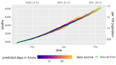
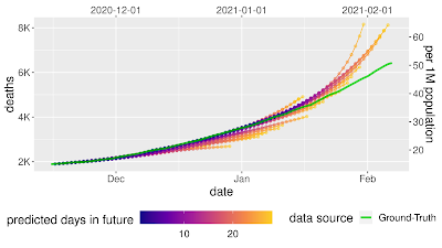
Prospective forecasts for the USA and Japan models. Ground truth cumulative deaths counts (green lines) are shown alongside the forecasts for each day. Each daily forecast contains a predicted increase in deaths for each day during the prediction window of 4 weeks (shown as colored dots, where shading shifting to yellow indicates days further from the date of prediction in the forecasting horizon, up to 4 weeks). Predictions of deaths are shown for the USA (above) and Japan (below).

The Model
Models for infectious diseases have been studied by epidemiologists for decades. Compartmental models are the most common, as they are simple, interpretable, and can fit different disease phases effectively. In compartmental models, individuals are separated into mutually exclusive groups, or compartments, based on their disease status (such as susceptible, exposed, or recovered), and the rates of change between these compartments are modeled to fit the past data. A population is assigned to compartments representing disease states, with people flowing between states as their disease status changes.

In this work, we propose a few extensions to the Susceptible-Exposed-Infectious-Removed (SEIR) type compartmental model. For example, susceptible people becoming exposed causes the susceptible compartment to decrease and the exposed compartment to increase, with a rate that depends on disease spreading characteristics. Observed data for COVID-19 associated outcomes, such as confirmed cases, hospitalizations and deaths, are used for training of compartmental models.

Visual explanation of "compartmental” models in epidemiology. People "flow" between compartments. Real-world events, like policy changes and more ICU beds, change the rate of flow between compartments.

Our framework proposes a number of novel technical innovations:

  1. Learned transition rates: Instead of using static rates for transitions between compartments across all locations and times, we use machine-learned rates to map them. This allows us to take advantage of the vast amount of available data with informative signals, such as Google's COVID-19 Community Mobility Reports, healthcare supply, demographics, and econometrics features.
  2. Explainability: Our framework provides explainability for decision makers, offering insights on disease propagation trends via its compartmental structure, and suggesting which factors may be most important for driving compartmental transitions.
  3. Expanded compartments: We add hospitalization, ICU, ventilator, and vaccine compartments and demonstrate efficient training despite data sparsity.
  4. Information sharing across locations: As opposed to fitting to an individual location, we have a single model for all locations in a country (e.g., >3000 US counties) with distinct dynamics and characteristics, and we show the benefit of transferring information across locations.
  5. Seq2seq modeling: We use a sequence-to-sequence model with a novel partial teacher forcing approach that minimizes amplified growth of errors into the future.

Forecast Accuracy
Each day, we train models to predict COVID-19 associated outcomes (primarily deaths and cases) 28 days into the future. We report the mean absolute percentage error (MAPE) for both a country-wide score and a location-level score, with both cumulative values and weekly incremental values for COVID-19 associated outcomes.

We compare our framework with alternatives for the US from the COVID19 Forecast Hub. In MAPE, our models outperform all other 33 models except one — the ensemble forecast that also includes our model’s predictions, where the difference is not statistically significant.

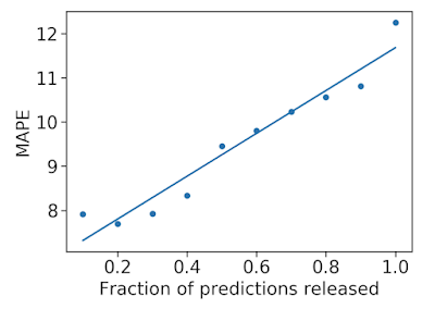
We also used prediction uncertainty to estimate whether a forecast is likely to be accurate. If we reject forecasts that the model considers uncertain, we can improve the accuracy of the forecasts that we do release. This is possible because our model has well-calibrated uncertainty.

Mean average percentage error (MAPE, the lower the better) decreases as we remove uncertain forecasts, increasing accuracy.

What-If Tool to Simulate Pandemic Management Policies and Strategies
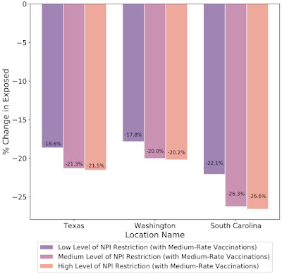
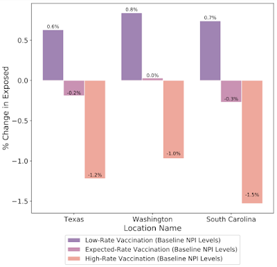
In addition to understanding the most probable scenario given past data, decision makers are interested in how different decisions could affect future outcomes, for example, understanding the impact of school closures, mobility restrictions and different vaccination strategies. Our framework allows counterfactual analysis by replacing the forecasted values for selected variables with their counterfactual counterparts. The results of our simulations reinforce the risk of prematurely relaxing non-pharmaceutical interventions (NPIs) until the rapid disease spreading is reduced. Similarly, the Japan simulations show that maintaining the State of Emergency while having a high vaccination rate greatly reduces infection rates.

What-if simulations on the percent change of predicted exposed individuals assuming different non-pharmaceutical interventions (NPIs) for the prediction date of March 1, 2021 in Texas, Washington and South Carolina. Increased NPI restrictions are associated with a larger % reduction in the number of exposed people.
What-if simulations on the percent change of predicted exposed individuals assuming different vaccination rates for the prediction date of March 1, 2021 in Texas, Washington and South Carolina. Increased vaccination rate also plays a key role to reduce exposed count in these cases.

Fairness Analysis
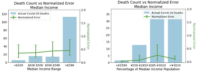
To ensure that our models do not create or reinforce unfairly biased decision making, in alignment with our AI Principles, we performed a fairness analysis separately for forecasts in the US and Japan by quantifying whether the model's accuracy was worse on protected sub-groups. These categories include age, gender, income, and ethnicity in the US, and age, gender, income, and country of origin in Japan. In all cases, we demonstrated no consistent pattern of errors among these groups once we controlled for the number of COVID-19 deaths and cases that occur in each subgroup.

Normalized errors by median income. The comparison between the two shows that patterns of errors don't persist once errors are normalized by cases. Left: Normalized errors by median income for the US. Right: Normalized errors by median income for Japan.

Real-World Use Cases
In addition to quantitative analyses to measure the performance of our models, we conducted a structured survey in the US and Japan to understand how organisations were using our model forecasts. In total, seven organisations responded with the following results on the applicability of the model.

  • Organization type: Academia (3), Government (2), Private industry (2)
  • Main user job role: Analyst/Scientist (3), Healthcare professional (1), Statistician (2), Managerial (1)
  • Location: USA (4), Japan (3)
  • Predictions used: Confirmed cases (7), Death (4), Hospitalizations (4), ICU (3), Ventilator (2), Infected (2)
  • Model use case: Resource allocation (2), Business planning (2), scenario planning (1), General understanding of COVID spread (1), Confirm existing forecasts (1)
  • Frequency of use: Daily (1), Weekly (1), Monthly (1)
  • Was the model helpful?: Yes (7)

To share a few examples, in the US, the Harvard Global Health Institute and Brown School of Public Health used the forecasts to help create COVID-19 testing targets that were used by the media to help inform the public. The US Department of Defense used the forecasts to help determine where to allocate resources, and to help take specific events into account. In Japan, the model was used to make business decisions. One large, multi-prefecture company with stores in more than 20 prefectures used the forecasts to better plan their sales forecasting, and to adjust store hours.

Limitations and next steps
Our approach has a few limitations. First, it is limited by available data, and we are only able to release daily forecasts as long as there is reliable, high-quality public data. For instance, public transportation usage could be very useful but that information is not publicly available. Second, there are limitations due to the model capacity of compartmental models as they cannot model very complex dynamics of Covid-19 disease propagation. Third, the distribution of case counts and deaths are very different between the US and Japan. For example, most of Japan's COVID-19 cases and deaths have been concentrated in a few of its 47 prefectures, with the others experiencing low values. This means that our per-prefecture models, which are trained to perform well across all Japanese prefectures, often have to strike a delicate balance between avoiding overfitting to noise while getting supervision from these relatively COVID-19-free prefectures.

We have updated our models to take into account large changes in disease dynamics, such as the increasing number of vaccinations. We are also expanding to new engagements with city governments, hospitals, and private organizations. We hope that our public releases continue to help public and policy-makers address the challenges of the ongoing pandemic, and we hope that our method will be useful to epidemiologists and public health officials in this and future health crises.

Acknowledgements
This paper was the result of hard work from a variety of teams within Google and collaborators around the globe. We'd especially like to thank our paper co-authors from the School of Medicine at Keio University, Graduate School of Public Health at St Luke’s International University, and Graduate School of Medicine at The University of Tokyo.

Source: Google AI Blog


Personalized ASR Models from a Large and Diverse Disordered Speech Dataset

Speech impairments affect millions of people, with underlying causes ranging from neurological or genetic conditions to physical impairment, brain damage or hearing loss. Similarly, the resulting speech patterns are diverse, including stuttering, dysarthria, apraxia, etc., and can have a detrimental impact on self-expression, participation in society and access to voice-enabled technologies. Automatic speech recognition (ASR) technologies have the potential to help individuals with such speech impairments by improving access to dictation and home automation and by enhancing communication. However, while the increased computational power of deep learning systems and the availability of large training datasets has improved the accuracy of ASR systems, their performance is still insufficient for many people with speech disorders, rendering the technology unusable for many of the speakers who could benefit the most.

In 2019, we introduced Project Euphonia and discussed how we could use personalized ASR models of disordered speech to achieve accuracies on par with non-personalized ASR on typical speech. Today we share the results of two studies, presented at Interspeech 2021, that aim to expand the availability of personalized ASR models to more users. In “Disordered Speech Data Collection: Lessons Learned at 1 Million Utterances from Project Euphonia”, we present a greatly expanded collection of disordered speech data, composed of over 1 million utterances. Then, in “Automatic Speech Recognition of Disordered Speech: Personalized models outperforming human listeners on short phrases”, we discuss our efforts to generate personalized ASR models based on this corpus. This approach leads to highly accurate models that can achieve up to 85% improvement to the word error rate in select domains compared to out-of-the-box speech models trained on typical speech.

Impaired Speech Data Collection
Since 2019, speakers with speech impairments of varying degrees of severity across a variety of conditions have provided voice samples to support Project Euphonia’s research mission. This effort has grown Euphonia’s corpus to over 1 million utterances, comprising over 1400 hours from 1330 speakers (as of August 2021).

Distribution of severity of speech disorder and condition across all speakers with more than 300 utterances recorded. For conditions, only those with > 5 speakers are shown (all others aggregated into “OTHER” for k-anonymity).
ALS = amyotrophic lateral sclerosis; DS = Down syndrome; PD = Parkinson’s disease; CP = cerebral palsy; HI = hearing impaired; MD = muscular dystrophy; MS = multiple sclerosis

To simplify the data collection, participants used an at-home recording system on their personal hardware (laptop or phone, with and without headphones), instead of an idealized lab-based setting that would collect studio quality recordings.

To reduce transcription cost, while still maintaining high transcript conformity, we prioritized scripted speech. Participants read prompts shown on a browser-based recording tool. Phrase prompts covered use-cases like home automation (“Turn on the TV.”), caregiver conversations (“I am hungry.”) and informal conversations (“How are you doing? Did you have a nice day?”). Most participants received a list of 1500 phrases, which included 1100 unique phrases along with 100 phrases that were each repeated four more times.

Speech professionals conducted a comprehensive auditory-perceptual speech assessment while listening to a subset of utterances for every speaker providing the following speaker-level metadata: speech disorder type (e.g., stuttering, dysarthria, apraxia), rating of 24 features of abnormal speech (e.g., hypernasality, articulatory imprecision, dysprosody), as well as recording quality assessments of both technical (e.g., signal dropouts, segmentation problems) and acoustic (e.g., environmental noise, secondary speaker crosstalk) features.

Personalized ASR Models
This expanded impaired speech dataset is the foundation of our new approach to personalized ASR models for disordered speech. Each personalized model uses a standard end-to-end, RNN-Transducer (RNN-T) ASR model that is fine-tuned using data from the target speaker only.

Architecture of RNN-Transducer. In our case, the encoder network consists of 8 layers and the predictor network consists of 2 layers of uni-directional LSTM cells.

To accomplish this, we focus on adapting the encoder network, i.e. the part of the model dealing with the specific acoustics of a given speaker, as speech sound disorders were most common in our corpus. We found that only updating the bottom five (out of eight) encoder layers while freezing the top three encoder layers (as well as the joint layer and decoder layers) led to the best results and effectively avoided overfitting. To make these models more robust against background noise and other acoustic effects, we employ a configuration of SpecAugment specifically tuned to the prevailing characteristics of disordered speech. Further, we found that the choice of the pre-trained base model was critical. A base model trained on a large and diverse corpus of typical speech (multiple domains and acoustic conditions) proved to work best for our scenario.

Results
We trained personalized ASR models for ~430 speakers who recorded at least 300 utterances. 10% of utterances were held out as a test set (with no phrase overlap) on which we calculated the word error rate (WER) for the personalized model and the unadapted base model.

Overall, our personalization approach yields significant improvements across all severity levels and conditions. Even for severely impaired speech, the median WER for short phrases from the home automation domain dropped from around 89% to 13%. Substantial accuracy improvements were also seen across other domains such as conversational and caregiver.

WER of unadapted and personalized ASR models on home automation phrases.

To understand when personalization does not work well, we analyzed several subgroups:

  • HighWER and LowWER: Speakers with high and low personalized model WERs based on the 1st and 5th quintiles of the WER distribution.
  • SurpHighWER: Speakers with a surprisingly high WER (participants with typical speech or mild speech impairment of the HighWER group).

Different pathologies and speech disorder presentations are expected to impact ASR non-uniformly. The distribution of speech disorder types within the HighWER group indicates that dysarthria due to cerebral palsy was particularly difficult to model. Not surprisingly, median severity was also higher in this group.

To identify the speaker-specific and technical factors that impact ASR accuracy, we examined the differences (Cohen's D) in the metadata between the participants that had poor (HighWER) and excellent (LowWER) ASR performance. As expected, overall speech severity was significantly lower in the LowWER group than in the HighWER group (p < 0.01). Intelligibility and severity were the most prominent atypical speech features in the HighWER group; however, other speech features also emerged, including abnormal prosody, articulation, and phonation. These speech features are known to degrade overall speech intelligibility.

The SurpHighWER group had fewer training utterances and lower SNR compared with the LowWER group (p < 0.01) resulting in large (negative) effect sizes, with all other factors having small effect sizes, except fastness. In contrast, the HighWER group exhibited medium to large differences across all factors.

Speech disorder and technical metadata effect sizes for the HighWER-vs-LowWER and SurpHighWER-vs-LowWER pairs. Positive effects indicated that the group values of the HighWER group were greater than LowWER groups.

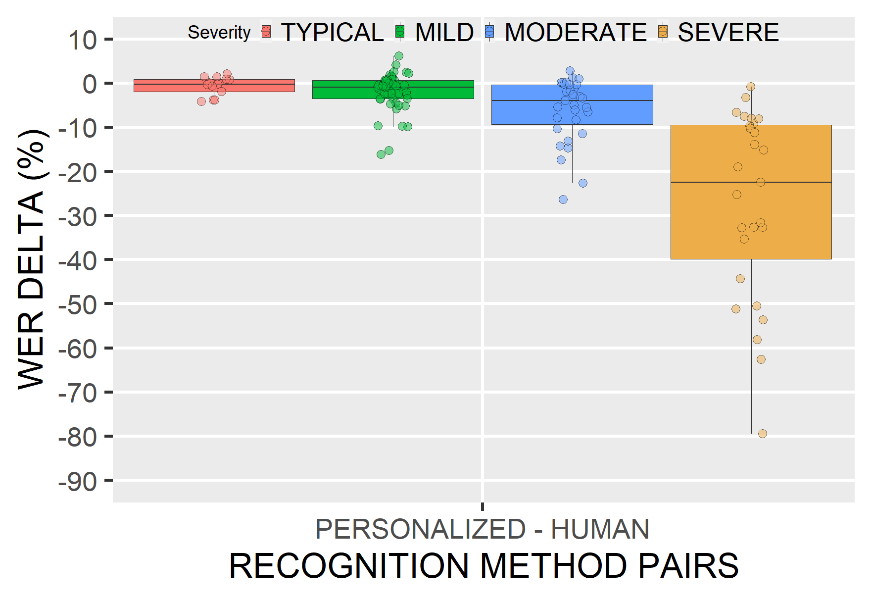
We then compared personalized ASR models to human listeners. Three speech professionals independently transcribed 30 utterances per speaker. We found that WERs were, on average, lower for personalized ASR models compared to the WERs of human listeners, with gains increasing by severity.

Delta between the WERs of the personalized ASR models and the human listeners. Negative values indicate that personalized ASR performs better than human (expert) listeners.

Conclusions
With over 1 million utterances, Euphonia’s corpus is one of the largest and most diversely disordered speech corpora (in terms of disorder types and severities) and has enabled significant advances in ASR accuracy for these types of atypical speech. Our results demonstrate the efficacy of personalized ASR models for recognizing a wide range of speech impairments and severities, with potential for making ASR available to a wider population of users.

Acknowledgements
Key contributors to this project include Michael Brenner, Julie Cattiau, Richard Cave, Jordan Green, Rus Heywood, Pan-Pan Jiang, Anton Kast, Marilyn Ladewig, Bob MacDonald, Phil Nelson, Katie Seaver, Jimmy Tobin, and Katrin Tomanek. We gratefully acknowledge the support Project Euphonia received from members of many speech research teams across Google, including Françoise Beaufays, Fadi Biadsy, Dotan Emanuel, Khe Chai Sim, Pedro Moreno Mengibar, Arun Narayanan, Hasim Sak, Suzan Schwartz, Joel Shor, and many others. And most importantly, we wanted to say a huge thank you to the over 1300 participants who recorded speech samples and the many advocacy groups who helped us connect with these participants.

Source: Google AI Blog


Recreating Natural Voices for People with Speech Impairments

On June 2nd, 2021, Major League Baseball in the United States celebrated Lou Gehrig Day, commemorating both the day in 1925 that Lou Gehrig became the Yankees’ starting first baseman, and the day in 1941 that he passed away from amyotrophic lateral sclerosis (ALS, also known as Lou Gehrig’s disease) at the age of 37. ALS is a progressive neurodegenerative disease that affects motor neurons, which connect the brain with the muscles throughout the body, and govern muscle control and voluntary movements. When voluntary muscle control is affected, people may lose their ability to speak, eat, move and breathe.

In honor of Lou Gehrig, former NFL player and ALS advocate Steve Gleason, who lost his ability to speak due to ALS, recited Gehrig’s famous “Luckiest Man” speech at the June 2nd event using a recreation of his voice generated by a machine learning (ML) model. Gleason’s voice recreation was developed in collaboration with Google’s Project Euphonia, which aims to empower people who have impaired speaking ability due to ALS to better communicate using their own voices.

Steve Gleason, who lost his voice to ALS, worked with Google’s Project Euphonia to generate a speech in his own voice in honor of Lou Gehrig. A portion of Gleason’s speech was broadcast in ballparks across the country during the 4th inning on June 2nd, 2021.

Today we describe PnG NAT, the model adopted by Project Euphonia to recreate Steve Gleason’s voice. PnG NAT is a new text-to-speech synthesis (TTS) model that merges two state-of-the-art technologies, PnG BERT and Non-Attentive Tacotron (NAT), into a single model. It demonstrates significantly better quality and fluency than previous technologies, and represents a promising approach that can be extended to a wider array of users.

Recreating a Voice
Non-Attentive Tacotron (NAT) is the successor to Tacotron 2, a sequence-to-sequence neural TTS model proposed in 2017. Tacotron 2 used an attention module to connect the input text sequence and the output speech spectrogram frame sequence, so that the model knows which part of the text to pay attention to when generating each time step of the synthesized speech spectrogram. Tacotron 2 was the first TTS model that was able to synthesize speech that sounds as natural as a person speaking. However, with extensive experimentation we discovered that there is a small probability that the model can suffer from robustness issues — such as babbling, repeating, or skipping part of the text — due to the inherent flexibility of the attention mechanism.

NAT improves upon Tacotron 2 by replacing the attention module with a duration-based upsampler, which predicts a duration for each input phoneme and upsamples the encoded phoneme representation so that the output length corresponds to the length of the predicted speech spectrogram. Such a change both resolves the robustness issue, and improves the naturalness of the synthesized speech. This approach also enables precise control of the speech duration for each phoneme of the input text while still maintaining highly natural synthesis quality. Because recordings of people with ALS often exhibit disfluent speech, this ability to exert per-phoneme control is key for achieving the fluency of the recreated voice.

Non-Attentive Tacotron (NAT) model.

While NAT addresses the robustness issue and enables precise duration control in neural TTS, we build upon it to further improve the natural language understanding of the TTS input. For this, we apply PnG BERT, which uses an approach similar to BERT, but is specifically designed for TTS. It is pre-trained with self-supervision on both the phoneme representation and the grapheme representation of the same content from a large text corpus, and then is used as the encoder of the TTS model. This results in a significant improvement of the prosody and pronunciation of the synthesized speech, especially in difficult cases.

Take, for example, the following audio, which was synthesized from a regular NAT model that takes only phonemes as input:

In comparison, the audio synthesized from PnG NAT on the same input text includes an additional pause that makes the meaning more clear.

The input text to both models is, “To cancel the payment, press one; or to continue, two.” Notice the different pause lengths before the ending “two” in the two versions. The word “two” in the version output by the regular NAT model could be confused for “too”. Because “too” and “two” have identical pronunciation (and thus the same phoneme representation), the regular NAT model does not understand which of the two is appropriate, and assumes it to be the word that more frequently follows a comma, “too”. In contrast, the PnG NAT model can more easily tell the difference, because it takes graphemes in addition to phonemes as input, and thus makes more appropriate pause.

The PnG NAT model integrates the pre-trained PnG BERT model as the encoder to the NAT model. The hidden representations output from the encoder are used by NAT to predict the duration of each phoneme, and are then upsampled to match the length of the audio spectrogram, as outlined above. In the final step, a non-attentive decoder converts the upsampled hidden representations into audio speech spectrograms, which are finally converted into audio waveforms by a neural vocoder.

PnG BERT and the pre-training objectives. Yellow boxes represent phonemes, and pink boxes represent graphemes.
PnG NAT: PnG BERT replaces the original encoder in the NAT model. The random masking for the Masked Language Model (MLM) pre-training is removed.

To recreate Steve Gleason’s voice, we first trained a PnG NAT model with recordings from 31 professional speakers, and then fine-tuned it with 30 minutes of Gleason’s recordings. Because these latter recordings were made after he was diagnosed with ALS, they exhibit signs of slurring. The fine tuned model was able to synthesize speech that sounds very similar to these recordings. However, because the symptoms of ALS were already present in Gleason’s speech, they exhibited some similar disfluencies.

To mitigate this, we leveraged the phoneme duration control of NAT as well as the model trained with professional speakers. We first predicted the durations of each phoneme for both a professional speaker and for Gleason, and then used the geometric mean of the two durations for each phoneme to guide the NAT output. As a result, the model is able to speak in Gleason’s voice, but more fluently than in the original recordings.

Here is the full version of the synthesized Lou Gehrig speech in Gleason’s voice:

Besides recreating voices for people with ALS, PnG NAT is also powering voices for a variety of customers through Google Cloud Custom Voice.

Project Euphonia
Of the millions of people around the world who have neurologic conditions that may impact their speech, such as ALS, cerebral palsy or Down syndrome, many may find it difficult to be understood, which can make face-to-face communication challenging. Using voice-activated technologies can be frustrating too, as they don’t always work reliably. Project Euphonia is a Google Research initiative focused on helping people with impaired speech be better understood. The team is researching ways to improve speech recognition for individuals with speech impairments (see recent blog post and segment in TODAY show), as well as customized text-to-speech technology (see Age of AI documentary featuring former NFL player Tim Shaw).

Acknowledgements
Many people across Google Research, Google Cloud and Consumer Apps, and Google Accessibility teams contributed to this project and the event, including Michael Brenner, Bob MacDonald, Heiga Zen, Yu Zhang, Jonathan Shen, Isaac Elias‎, Yonghui Wu, Anne Keck, Danielle Notaro, Kevin Hogan, Zack Kaplan, KR Liu, Kyndra Price, Zoe Ortiz.

Source: Google AI Blog


Mapping Africa’s Buildings with Satellite Imagery

An accurate record of building footprints is important for a range of applications, from population estimation and urban planning to humanitarian response and environmental science. After a disaster, such as a flood or an earthquake, authorities need to estimate how many households have been affected. Ideally there would be up-to-date census information for this, but in practice such records may be out of date or unavailable. Instead, data on the locations and density of buildings can be a valuable alternative source of information.

A good way to collect such data is through satellite imagery, which can map the distribution of buildings across the world, particularly in areas that are isolated or difficult to access. However, detecting buildings with computer vision methods in some environments can be a challenging task. Because satellite imaging involves photographing the earth from several hundred kilometres above the ground, even at high resolution (30–50 cm per pixel), a small building or tent shelter occupies only a few pixels. The task is even more difficult for informal settlements, or rural areas where buildings constructed with natural materials can visually blend into the surroundings. There are also many types of natural and artificial features that can be easily confused with buildings in overhead imagery.

Objects that can confuse computer vision models for building identification (clockwise from top left) pools, rocks, enclosure walls and shipping containers.

In “Continental-Scale Building Detection from High-Resolution Satellite Imagery”, we address these challenges, using new methods for detecting buildings that work in rural and urban settings across different terrains, such as savannah, desert, and forest, as well as informal settlements and refugee facilities. We use this building detection model to create the Open Buildings dataset, a new open-access data resource containing the locations and footprints of 516 million buildings with coverage across most of the African continent. The dataset will support several practical, scientific and humanitarian applications, ranging from disaster response or population mapping to planning services such as new medical facilities or studying human impact on the natural environment.

Model Development
We built a training dataset for the building detection model by manually labelling 1.75 million buildings in 100k images. The figure below shows some examples of how we labelled images in the training data, taking into account confounding characteristics of different areas across the African continent. In rural areas, for example, it was necessary to identify different types of dwelling places and to disambiguate them from natural features, while in urban areas we needed to develop labelling policies for dense and contiguous structures.

(1) Example of a compound containing both dwelling places as well as smaller outbuildings such as grain stores. (2) Example of a round, thatched-roof structure that can be difficult for a model to distinguish from trees, and where it is necessary to use cues from pathways, clearings and shadows to disambiguate. (3) Example of several contiguous buildings for which the boundaries cannot be easily distinguished.

We trained the model to detect buildings in a bottom-up way, first by classifying each pixel as building or non-building, and then grouping these pixels together into individual instances. The detection pipeline was based on the U-Net model, which is commonly used in satellite image analysis. One advantage of U-Net is that it is a relatively compact architecture, and so can be applied to large quantities of imaging data without a heavy compute burden. This is critical, because the final task of applying this to continental-scale satellite imagery means running the model on many billions of image tiles.

Example of segmenting buildings in satellite imagery. Left: Source image; Center: Semantic segmentation, with each pixel assigned a confidence score that it is a building vs. non-building; Right: Instance segmentation, obtained by thresholding and grouping together connected components.

Initial experiments with the basic model had low precision and recall, for example due to the variety of natural and artificial features with building-like appearance. We found a number of methods that improved performance. One was the use of mixup as a regularisation method, where random training images are blended together by taking a weighted average. Though mixup was originally proposed for image classification, we modified it to be used for semantic segmentation. Regularisation is important in general for this building segmentation task, because even with 100k training images, the training data do not capture the full variation of terrain, atmospheric and lighting conditions that the model is presented with at test time, and hence, there is a tendency to overfit. This is mitigated by mixup as well as random augmentation of training images.

Another method that we found to be effective was the use of unsupervised self-training. We prepared a set of 100 million satellite images from across Africa, and filtered these to a subset of 8.7 million images that mostly contained buildings. This dataset was used for self-training using the Noisy Student method, in which the output of the best building detection model from the previous stage is used as a ‘teacher’ to then train a ‘student’ model that makes similar predictions from augmented images. In practice, we found that this reduced false positives and sharpened the detection output. The student model gave higher confidence to buildings and lower confidence to background.

Difference in model output between the student and teacher models for a typical image. In panel (d), red areas are those that the student model finds more likely to be buildings than the teacher model, and blue areas more likely to be background.

One problem that we faced initially was that our model had a tendency to create “blobby” detections, without clearly delineated edges and with a tendency for neighbouring buildings to be merged together. To address this, we applied another idea from the original U-Net paper, which is to use distance weighting to adapt the loss function to emphasise the importance of making correct predictions near boundaries. During training, distance weighting places greater emphasis at the edges by adding weight to the loss — particularly where there are instances that nearly touch. For building detection, this encourages the model to correctly identify the gaps in between buildings, which is important so that many close structures are not merged together. We found that the original U-Net distance weighting formulation was helpful but slow to compute. So, we developed an alternative based on Gaussian convolution of edges, which was both faster and more effective.

Distance weighting schemes to emphasise nearby edges: U-Net (left) and Gaussian convolution of edges (right).

Our technical report has more details on each of these methods.

Results
We evaluated the performance of the model on several different regions across the continent, in different categories: urban, rural, and medium-density. In addition, with the goal of preparing for potential humanitarian applications, we tested the model on regions with displaced persons and refugee settlements. Precision and recall did vary between regions, so achieving consistent performance across the continent is an ongoing challenge.

Precision-recall curves, measured at 0.5 intersection-over-union threshold.

When visually inspecting the detections for low-scoring regions, we noted various causes. In rural areas, label errors were problematic. For example, single buildings within a mostly-empty area can be difficult for labellers to spot. In urban areas, the model had a tendency to split large buildings into separate instances. The model also underperformed in desert terrain, where buildings were hard to distinguish against the background.

We carried out an ablation study to understand which methods contributed most to the final performance, measured in mean average precision (mAP). Distance weighting, mixup and the use of ImageNet pre-training were the biggest factors for the performance of the supervised learning baseline. The ablated models that did not use these methods had a mAP difference of -0.33, -0.12 and -0.07 respectively. Unsupervised self-training gave a further significant boost of +0.06 mAP.

Ablation study of training methods. The first row shows the mAP performance of the best model combined with self-training, and the second row shows the best model with supervised learning only (the baseline). By disabling each training optimization from the baseline in turn, we observe the impact on mAP test performance. Distance weighting has the most significant effect.

Generating the Open Buildings Dataset
To create the final dataset, we applied our best building detection model to satellite imagery across the African continent (8.6 billion image tiles covering 19.4 million km2, 64% of the continent), which resulted in the detection of 516M distinct structures.

Each building’s outline was simplified as a polygon and associated with a Plus Code, which is a geographic identifier made up of numbers and letters, akin to a street address, and useful for identifying buildings in areas that don’t have formal addressing systems. We also include confidence scores and guidance on suggested thresholds to achieve particular precision levels.

The sizes of the structures vary as shown below, tending towards small footprints. The inclusion of small structures is important, for example, to support analyses of informal settlements or refugee facilities.

Distribution of building footprint sizes.

The data is freely available and we look forward to hearing how it is used. In the future, we may add new features and regions, depending on usage and feedback.

Acknowledgements
This work is part of our AI for Social Good efforts and was led by Google Research, Ghana. Thanks to the co-authors of this work: Wojciech Sirko, Sergii Kashubin, Marvin Ritter, Abigail Annkah, Yasser Salah Edine Bouchareb, Yann Dauphin, Daniel Keysers, Maxim Neumann and Moustapha Cisse. We are grateful to Abdoulaye Diack, Sean Askay, Ruth Alcantara and Francisco Moneo for help with coordination. Rob Litzke, Brian Shucker, Yan Mayster and Michelina Pallone provided valuable assistance with geo infrastructure.

Source: Google AI Blog


Project Guideline: Enabling Those with Low Vision to Run Independently

For the 285 million people around the world living with blindness or low vision, exercising independently can be challenging. Earlier this year, we announced Project Guideline, an early-stage research project, developed in partnership with Guiding Eyes for the Blind, that uses machine learning to guide runners through a variety of environments that have been marked with a painted line. Using only a phone running Guideline technology and a pair of headphones, Guiding Eyes for the Blind CEO Thomas Panek was able to run independently for the first time in decades and complete an unassisted 5K in New York City’s Central Park.

Safely and reliably guiding a blind runner in unpredictable environments requires addressing a number of challenges. Here, we will walk through the technology behind Guideline and the process by which we were able to create an on-device machine learning model that could guide Thomas on an independent outdoor run. The project is still very much under development, but we’re hopeful it can help explore how on-device technology delivered by a mobile phone can provide reliable, enhanced mobility and orientation experiences for those who are blind or low vision.

Thomas Panek using Guideline technology to run independently outdoors.

Project Guideline
The Guideline system consists of a mobile device worn around the user’s waist with a custom belt and harness, a guideline on the running path marked with paint or tape, and bone conduction headphones. Core to the Guideline technology is an on-device segmentation model that takes frames from a mobile device’s camera as input and classifies every pixel in the frame into two classes, “guideline” and “not guideline”. This simple confidence mask, applied to every frame, allows the Guideline app to predict where runners are with respect to a line on the path, without using location data. Based on this prediction and the proceeding smoothing/filtering function, the app sends audio signals to the runners to help them orient and stay on the line, or audio alerts to tell runners to stop if they veer too far away.

Project Guideline uses Android’s built-in Camera 2 and MLKit APIs and adds custom modules to segment the guideline, detect its position and orientation, filter false signals, and send a stereo audio signal to the user in real-time.

We faced a number of important challenges in building the preliminary Guideline system:

  1. System accuracy: Mobility for the blind and low vision community is a challenge in which user safety is of paramount importance. It demands a machine learning model that is capable of generating accurate and generalized segmentation results to ensure the safety of the runner in different locations and under various environmental conditions.
  2. System performance: In addition to addressing user safety, the system needs to be performative, efficient, and reliable. It must process at least 15 frames per second (FPS) in order to provide real-time feedback for the runner. It must also be able to run for at least 3 hours without draining the phone battery, and must work offline, without the need for internet connection should the walking/running path be in an area without data service.
  3. Lack of in-domain data: In order to train the segmentation model, we needed a large volume of video consisting of roads and running paths that have a yellow line on them. To generalize the model, data variety is equally as critical as data quantity, requiring video frames taken at different times of day, with different lighting conditions, under different weather conditions, at different locations, etc.

Below, we introduce solutions for each of these challenges.

Network Architecture
To meet the latency and power requirements, we built the line segmentation model on the DeepLabv3 framework, utilizing MobilenetV3-Small as the backbone, while simplifying the outputs to two classes – guideline and background.

The model takes an RGB frame and generates an output grayscale mask, representing the confidence of each pixel’s prediction.

To increase throughput speed, we downsize the camera feed from 1920 x 1080 pixels to 513 x 513 pixels as input to the DeepLab segmentation model. To further speed-up the DeepLab model for use on mobile devices, we skipped the last up-sample layer, and directly output the 65 x 65 pixel predicted masks. These 65 x 65 pixel predicted masks are provided as input to the post processing. By minimizing the input resolution in both stages, we’re able to improve the runtime of the segmentation model and speed up post-processing.

Data Collection
To train the model, we required a large set of training images in the target domain that exhibited a variety of path conditions. Not surprisingly, the publicly available datasets were for autonomous driving use cases, with roof mounted cameras and cars driving between the lines, and were not in the target domain. We found that training models on these datasets delivered unsatisfying results due to the large domain gap. Instead, the Guideline model needed data collected with cameras worn around a person’s waist, running on top of the line, without the adversarial objects found on highways and crowded city streets.

The large domain gap between autonomous driving datasets and the target domain. Images on the left courtesy of the Berkeley DeepDrive dataset.

With preexisting open-source datasets proving unhelpful for our use case, we created our own training dataset composed of the following:

  1. Hand-collected data: Team members temporarily placed guidelines on paved pathways using duct tape in bright colors and recorded themselves running on and around the lines at different times of the day and in different weather conditions.
  2. Synthetic data: The data capture efforts were complicated and severely limited due to COVID-19 restrictions. This led us to build a custom rendering pipeline to synthesize tens of thousands of images, varying the environment, weather, lighting, shadows, and adversarial objects. When the model struggled with certain conditions in real-world testing, we were able to generate specific synthetic datasets to address the situation. For example, the model originally struggled with segmenting the guideline amidst piles of fallen autumn leaves. With additional synthetic training data, we were able to correct for that in subsequent model releases.
Rendering pipeline generates synthetic images to capture a broad spectrum of environments.

We also created a small regression dataset, which consisted of annotated samples of the most frequently seen scenarios combined with the most challenging scenarios, including tree and human shadows, fallen leaves, adversarial road markings, sunlight reflecting off the guideline, sharp turns, steep slopes, etc. We used this dataset to compare new models to previous ones and to make sure that an overall improvement in accuracy of the new model did not hide a reduction in accuracy in particularly important or challenging scenarios.

Training Procedure
We designed a three-stage training procedure and used transfer learning to overcome the limited in-domain training dataset problem. We started with a model that was pre-trained on Cityscape, and then trained the model using the synthetic images, as this dataset is larger but of lower quality. Finally, we fine-tuned the model using the limited in-domain data we collected.

Three-stage training procedure to overcome the limited data issue. Images in the left column courtesy of Cityscapes.

Early in development, it became clear that the segmentation model's performance suffered at the top of the image frame. As the guidelines travel further away from the camera’s point of view at the top of the frame, the lines themselves start to vanish. This causes the predicted masks to be less accurate at the top parts of the frame. To address this problem, we computed a loss value that was based on the top k pixel rows in every frame. We used this value to select those frames that included the vanishing guidelines with which the model struggled, and trained the model repeatedly on those frames. This process proved to be very helpful not only in addressing the vanishing line problem, but also for solving other problems we encountered, such as blurry frames, curved lines and line occlusion by adversarial objects.

The segmentation model’s accuracy and robustness continuously improved even in challenging cases.

System Performance
Together with Tensorflow Lite and ML Kit, the end-to-end system runs remarkably fast on Pixel devices, achieving 29+ FPS on Pixel 4 XL and 20+ FPS on Pixel 5. We deployed the segmentation model entirely on DSP, running at 6 ms on Pixel 4 XL and 12 ms on Pixel 5 with high accuracy. The end-to-end system achieves 99.5% frame success rate, 93% mIoU on our evaluation dataset, and passes our regression test. These model performance metrics are incredibly important and enable the system to provide real-time feedback to the user.

What's Next
We’re still at the beginning of our exploration, but we’re excited about our progress and what’s to come. We’re starting to collaborate with additional leading non-profit organizations that serve the blind and low vision communities to put more Guidelines in parks, schools, and public places. By painting more lines, getting direct feedback from users, and collecting more data under a wider variety of conditions, we hope to further generalize our segmentation model and improve the existing feature-set. At the same time, we are investigating new research and techniques, as well as new features and capabilities that would improve the overall system robustness and reliability.

To learn more about the project and how it came to be, read Thomas Panek’s story. If you want to help us put more Guidelines in the world, please visit goo.gle/ProjectGuideline.

Acknowledgements
Project Guideline is a collaboration across Google Research, Google Creative Lab, and the Accessibility Team. We especially would like to thank our team members: Mikhail Sirotenko, Sagar Waghmare, Lucian Lonita, Tomer Meron, Hartwig Adam, Ryan Burke, Dror Ayalon, Amit Pitaru, Matt Hall, John Watkinson, Phil Bayer, John Mernacaj, Cliff Lungaretti, Dorian Douglass, Kyndra LoCoco. We also thank Fangting Xia, Jack Sim and our other colleagues and friends from the Mobile Vision team and Guiding Eyes for the Blind.

Source: Google AI Blog