Category Archives: Research Blog

The latest news on Google Research

An ML-based approach to better characterize lung diseases

The combination of the environment an individual experiences and their genetic predispositions determines the majority of their risk for various diseases. Large national efforts, such as the UK Biobank, have created large, public resources to better understand the links between environment, genetics, and disease. This has the potential to help individuals better understand how to stay healthy, clinicians to treat illnesses, and scientists to develop new medicines.

One challenge in this process is how we make sense of the vast amount of clinical measurements — the UK Biobank has many petabytes of imaging, metabolic tests, and medical records spanning 500,000 individuals. To best use this data, we need to be able to represent the information present as succinct, informative labels about meaningful diseases and traits, a process called phenotyping. That is where we can use the ability of ML models to pick up on subtle intricate patterns in large amounts of data.

We’ve previously demonstrated the ability to use ML models to quickly phenotype at scale for retinal diseases. Nonetheless, these models were trained using labels from clinician judgment, and access to clinical-grade labels is a limiting factor due to the time and expense needed to create them.

In “Inference of chronic obstructive pulmonary disease with deep learning on raw spirograms identifies new genetic loci and improves risk models”, published in Nature Genetics, we’re excited to highlight a method for training accurate ML models for genetic discovery of diseases, even when using noisy and unreliable labels. We demonstrate the ability to train ML models that can phenotype directly from raw clinical measurement and unreliable medical record information. This reduced reliance on medical domain experts for labeling greatly expands the range of applications for our technique to a panoply of diseases and has the potential to improve their prevention, diagnosis, and treatment. We showcase this method with ML models that can better characterize lung function and chronic obstructive pulmonary disease (COPD). Additionally, we show the usefulness of these models by demonstrating a better ability to identify genetic variants associated with COPD, improved understanding of the biology behind the disease, and successful prediction of outcomes associated with COPD.


ML for deeper understanding of exhalation

For this demonstration, we focused on COPD, the third leading cause of worldwide death in 2019, in which airway inflammation and impeded airflow can progressively reduce lung function. Lung function for COPD and other diseases is measured by recording an individual’s exhalation volume over time (the record is called a spirogram; see an example below). Although there are guidelines (called GOLD) for determining COPD status from exhalation, these use only a few, specific data points in the curve and apply fixed thresholds to those values. Much of the rich data from these spirograms is discarded in this analysis of lung function.

We reasoned that ML models trained to classify spirograms would be able to use the rich data present more completely and result in more accurate and comprehensive measures of lung function and disease, similar to what we have seen in other classification tasks like mammography or histology. We trained ML models to predict whether an individual has COPD using the full spirograms as inputs.

Spirometry and COPD status overview. Spirograms from lung function test showing a forced expiratory volume-time spirogram (left), a forced expiratory flow-time spirogram (middle), and an interpolated forced expiratory flow-volume spirogram (right). The profile of individuals w/o COPD is different.

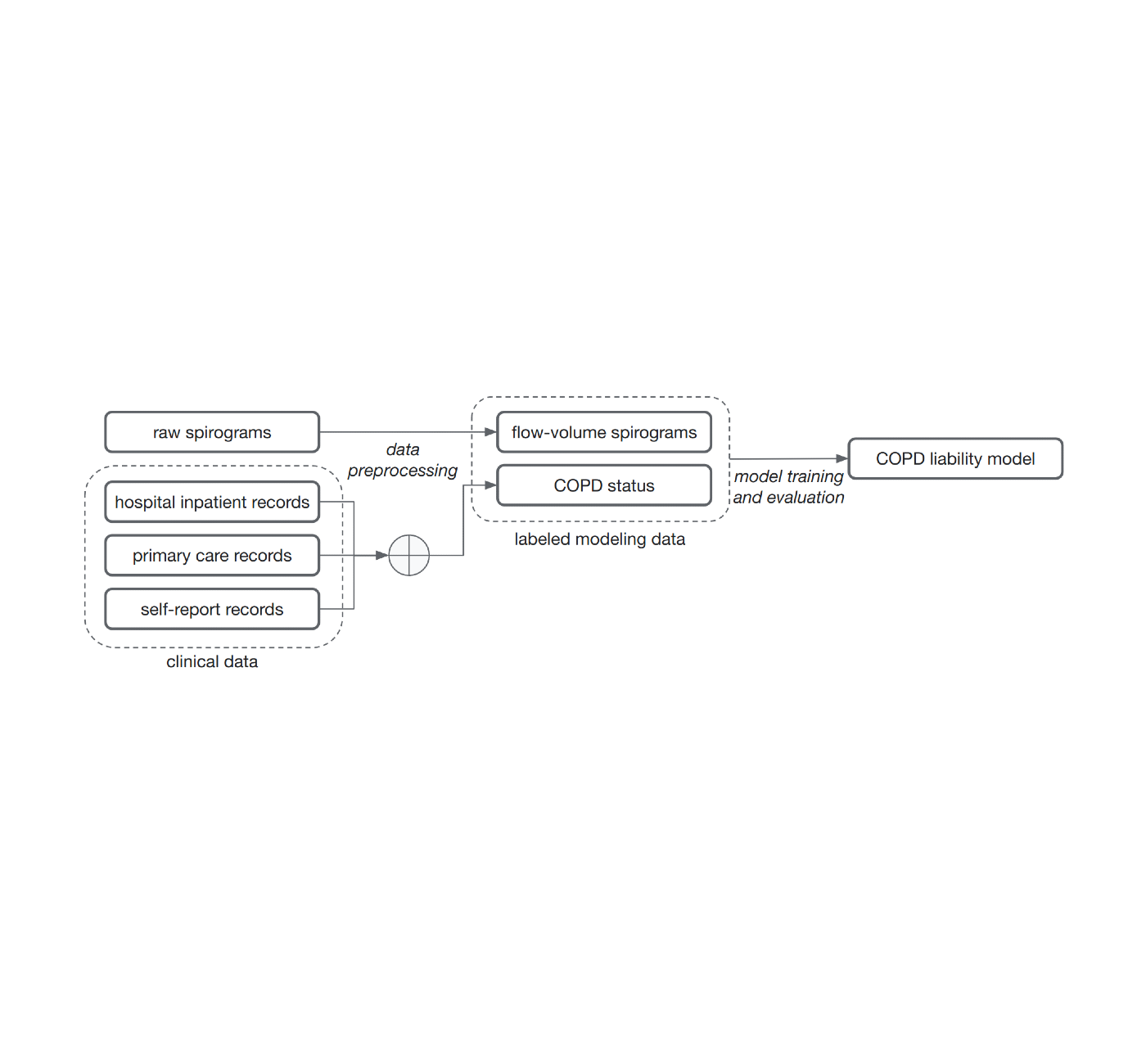
The common method of training models for this problem, supervised learning, requires samples to be associated with labels. Determining those labels can require the effort of very time-constrained experts. For this work, to show that we do not necessarily need medically graded labels, we decided to use a variety of widely available sources of medical record information to create those labels without medical expert review. These labels are less reliable and noisy for two reasons. First, there are gaps in the medical records of individuals because they use multiple health services. Second, COPD is often undiagnosed, meaning many with the disease will not be labeled as having it even if we compile the complete medical records. Nonetheless, we trained a model to predict these noisy labels from the spirogram curves and treat the model predictions as a quantitative COPD liability or risk score.

Noisy COPD status labels were derived using various medical record sources (clinical data). A COPD liability model is then trained to predict COPD status from raw flow-volume spirograms.

Predicting COPD outcomes

We then investigated whether the risk scores produced by our model could better predict a variety of binary COPD outcomes (for example, an individual’s COPD status, whether they were hospitalized for COPD or died from it). For comparison, we benchmarked the model relative to expert-defined measurements required to diagnose COPD, specifically FEV1/FVC, which compares specific points on the spirogram curve with a simple mathematical ratio. We observed an improvement in the ability to predict these outcomes as seen in the precision-recall curves below.

Precision-recall curves for COPD status and outcomes for our ML model (green) compared to traditional measures. Confidence intervals are shown by lighter shading.

We also observed that separating populations by their COPD model score was predictive of all-cause mortality. This plot suggests that individuals with higher COPD risk are more likely to die earlier from any causes and the risk probably has implications beyond just COPD.

Survival analysis of a cohort of UK Biobank individuals stratified by their COPD model’s predicted risk quartile. The decrease of the curve indicates individuals in the cohort dying over time. For example, p100 represents the 25% of the cohort with greatest predicted risk, while p50 represents the 2nd quartile.

Identifying the genetic links with COPD

Since the goal of large scale biobanks is to bring together large amounts of both phenotype and genetic data, we also performed a test called a genome-wide association study (GWAS) to identify the genetic links with COPD and genetic predisposition. A GWAS measures the strength of the statistical association between a given genetic variant — a change in a specific position of DNA — and the observations (e.g., COPD) across a cohort of cases and controls. Genetic associations discovered in this manner can inform drug development that modifies the activity or products of a gene, as well as expand our understanding of the biology for a disease.

We showed with our ML-phenotyping method that not only do we rediscover almost all known COPD variants found by manual phenotyping, but we also find many novel genetic variants significantly associated with COPD. In addition, we see good agreement on the effect sizes for the variants discovered by both our ML approach and the manual one (R2=0.93), which provides strong evidence for validity of the newly found variants.

Left: A plot comparing the statistical power of genetic discovery using the labels for our ML model (y-axis) with the statistical power of the manual labels from a traditional study (x-axis). A value above the y = x line indicates greater statistical power in our method. Green points indicate significant findings in our method that are not found using the traditional approach. Orange points are significant in the traditional approach but not ours. Blue points are significant in both. Right: Estimates of the association effect between our method (y-axis) and traditional method (x-axis). Note that the relative values between studies are comparable but the absolute numbers are not.

Finally, our collaborators at Harvard Medical School and Brigham and Women’s Hospital further examined the plausibility of these findings by providing insights into the possible biological role of the novel variants in development and progression of COPD (you can see more discussion on these insights in the paper).


Conclusion

We demonstrated that our earlier methods for phenotyping with ML can be expanded to a wide range of diseases and can provide novel and valuable insights. We made two key observations by using this to predict COPD from spirograms and discovering new genetic insights. First, domain knowledge was not necessary to make predictions from raw medical data. Interestingly, we showed the raw medical data is probably underutilized and the ML model can find patterns in it that are not captured by expert-defined measurements. Second, we do not need medically graded labels; instead, noisy labels defined from widely available medical records can be used to generate clinically predictive and genetically informative risk scores. We hope that this work will broadly expand the ability of the field to use noisy labels and will improve our collective understanding of lung function and disease.


Acknowledgments

This work is the combined output of multiple contributors and institutions. We thank all contributors: Justin Cosentino, Babak Alipanahi, Zachary R. McCaw, Cory Y. McLean, Farhad Hormozdiari (Google), Davin Hill (Northeastern University), Tae-Hwi Schwantes-An and Dongbing Lai (Indiana University), Brian D. Hobbs and Michael H. Cho (Brigham and Women’s Hospital, and Harvard Medical School). We also thank Ted Yun and Nick Furlotte for reviewing the manuscript, Greg Corrado and Shravya Shetty for support, and Howard Yang, Kavita Kulkarni, and Tammi Huynh for helping with publication logistics.

Source: Google AI Blog


Robust and efficient medical imaging with self-supervision

Despite recent progress in the field of medical artificial intelligence (AI), most existing models are narrow, single-task systems that require large quantities of labeled data to train. Moreover, these models cannot be easily reused in new clinical contexts as they often require the collection, de-identification and annotation of site-specific data for every new deployment environment, which is both laborious and expensive. This problem of data-efficient generalization (a model’s ability to generalize to new settings using minimal new data) continues to be a key translational challenge for medical machine learning (ML) models and has in turn, prevented their broad uptake in real world healthcare settings.

The emergence of foundation models offers a significant opportunity to rethink development of medical AI to make it more performant, safer, and equitable. These models are trained using data at scale, often by self-supervised learning. This process results in generalist models that can rapidly be adapted to new tasks and environments with less need for supervised data. With foundation models, it may be possible to safely and efficiently deploy models across various clinical contexts and environments.

In “Robust and Efficient MEDical Imaging with Self-supervision” (REMEDIS), to be published in Nature Biomedical Engineering, we introduce a unified large-scale self-supervised learning framework for building foundation medical imaging models. This strategy combines large scale supervised transfer learning with self-supervised learning and requires minimal task-specific customization. REMEDIS shows significant improvement in data-efficient generalization across medical imaging tasks and modalities with a 3–100x reduction in site-specific data for adapting models to new clinical contexts and environments. Building on this, we are excited to announce Medical AI Research Foundations (hosted by PhysioNet), an expansion of the public release of chest X-ray Foundations in 2022. Medical AI Research Foundations is a collection of open-source non-diagnostic models (starting with REMEDIS models), APIs, and resources to help researchers and developers accelerate medical AI research.


Large scale self-supervision for medical imaging

REMEDIS uses a combination of natural (non-medical) images and unlabeled medical images to develop strong medical imaging foundation models. Its pre-training strategy consists of two steps. The first involves supervised representation learning on a large-scale dataset of labeled natural images (pulled from Imagenet 21k or JFT) using the Big Transfer (BiT) method.

The second step involves intermediate self-supervised learning, which does not require any labels and instead, trains a model to learn medical data representations independently of labels. The specific approach used for pre-training and learning representations is SimCLR. The method works by maximizing agreement between differently augmented views of the same training example via a contrastive loss in a hidden layer of a feed-forward neural network with multilayer perceptron (MLP) outputs. However, REMEDIS is equally compatible with other contrastive self-supervised learning methods. This training method is applicable for healthcare environments as many hospitals acquire raw data (images) as a routine practice. While processes would have to be implemented to make this data usable within models (i.e., patient consent prior to gathering the data, de-identification, etc.), the costly, time-consuming, and difficult task of labeling that data could be avoided using REMEDIS.

REMEDIS leverages large-scale supervised learning using natural images and self-supervised learning using unlabeled medical data to create strong foundation models for medical imaging.

Given ML model parameter constraints, it is important that our proposed approach works when using both small and large model architecture sizes. To study this in detail, we considered two ResNet architectures with commonly used depth and width multipliers, ResNet-50 (1×) and ResNet-152 (2×) as the backbone encoder networks.

After pre-training, the model was fine-tuned using labeled task-specific medical data and evaluated for in-distribution task performance. In addition, to evaluate the data-efficient generalization, the model was also optionally fine-tuned using small amounts of out-of-distribution (OOD) data.

REMEDIS starts with representations initialized using large-scale natural image pretraining following the Big Transfer (BiT) method. We then adapt the model to the medical domain using intermediate contrastive self-supervised learning without using any labeled medical data. Finally, we fine-tune the model to specific downstream medical imaging tasks. We evaluate the ML model both in an in-distribution (ID) setting and in an out-of-distribution (OOD) setting to establish the data-efficient generalization performance of the model.

Evaluation and results

To evaluate the REMEDIS model’s performance, we simulate realistic scenarios using retrospective de-identified data across a broad range of medical imaging tasks and modalities, including dermatology, retinal imaging, chest X-ray interpretation, pathology and mammography. We further introduce the notion of data-efficient generalization, capturing the model’s ability to generalize to new deployment distributions with a significantly reduced need for expert annotated data from the new clinical setting. In-distribution performance is measured as (1) improvement in zero-shot generalization to OOD settings (assessing performance in an OOD evaluation set, with zero access to training data from the OOD dataset) and (2) significant reduction in the need for annotated data from the OOD settings to reach performance equivalent to clinical experts (or threshold demonstrating clinical utility). REMEDIS exhibits significantly improved in-distribution performance with up to 11.5% relative improvement in diagnostic accuracy over a strongly supervised baseline.

More importantly, our strategy leads to data-efficient generalization of medical imaging models, matching strong supervised baselines resulting in a 3–100x reduction in the need for retraining data. While SimCLR is the primary self-supervised learning approach used in the study, we also show that REMEDIS is compatible with other approaches, such as MoCo-V2, RELIC and Barlow Twins. Furthermore, the approach works across model architecture sizes.

REMEDIS outperformed the supervised baseline pre-trained on JFT-300M for various medical tasks and demonstrated improved data-efficient generalization, reducing data needs by 3–100x for adapting models to new clinical settings. This could potentially translate to significant reduction in clinician hours saved annotating data and cost of developing robust medical imaging systems.
REMEDIS is compatible with MoCo-V2, RELIC and Barlow Twins as alternate self-supervised learning strategies. All the REMEDIS variants lead to data-efficient generalization improvements over the strong supervised baseline for dermatology condition classification (T1), diabetic macular edema classification (T2), and chest X-ray condition classification (T3). The gray shaded area indicates the performance of the strong supervised baseline pre-trained on JFT.

Medical AI Research Foundations

Building on REMEDIS, we are excited to announce Medical AI Research Foundations, an expansion of the public release of chest X-ray Foundations in 2022. Medical AI Research Foundations is a repository of open-source medical foundation models hosted by PhysioNet. This expands the previous API-based approach to also encompass non-diagnostic models, to help researchers and developers accelerate their medical AI research. We believe that REMEDIS and the release of the Medical AI Research Foundations are a step toward building medical models that can generalize across healthcare settings and tasks.

We are seeding Medical AI Research Foundations with REMEDIS models for chest X-ray and pathology (with related code). Whereas the existing chest X-ray Foundation approach focuses on providing frozen embeddings for application-specific fine tuning from a model trained on several large private datasets, the REMEDIS models (trained on public datasets) enable users to fine-tune end-to-end for their application, and to run on local devices. We recommend users test different approaches based on their unique needs for their desired application. We expect to add more models and resources for training medical foundation models such as datasets and benchmarks in the future. We also welcome the medical AI research community to contribute to this.


Conclusion

These results suggest that REMEDIS has the potential to significantly accelerate the development of ML systems for medical imaging, which can preserve their strong performance when deployed in a variety of changing contexts. We believe this is an important step forward for medical imaging AI to deliver a broad impact. Beyond the experimental results presented, the approach and insights described here have been integrated into several of Google’s medical imaging research projects, such as dermatology, mammography and radiology among others. We’re using a similar self-supervised learning approach with our non-imaging foundation model efforts, such as Med-PaLM and Med-PaLM 2.

With REMEDIS, we demonstrated the potential of foundation models for medical imaging applications. Such models hold exciting possibilities in medical applications with the opportunity of multimodal representation learning. The practice of medicine is inherently multimodal and incorporates information from images, electronic health records, sensors, wearables, genomics and more. We believe ML systems that leverage these data at scale using self-supervised learning with careful consideration of privacy, safety, fairness and ethics will help lay the groundwork for the next generation of learning health systems that scale world-class healthcare to everyone.


Acknowledgements

This work involved extensive collaborative efforts from a multidisciplinary team of researchers, software engineers, clinicians, and cross-functional contributors across Google Health AI and Google Brain. In particular, we would like to thank our first co-author Jan Freyberg and our lead senior authors of these projects, Vivek Natarajan, Alan Karthikesalingam, Mohammad Norouzi and Neil Houlsby for their invaluable contributions and support. We also thank Lauren Winer, Sami Lachgar, Yun Liu and Karan Singhal for their feedback on this post and Tom Small for support in creating the visuals. Finally, we also thank the PhysioNet team for their support on hosting Medical AI Research Foundations. Users with questions can reach out to medical-ai-research-foundations at google.com.

Source: Google AI Blog


LayerNAS: Neural Architecture Search in Polynomial Complexity

Every byte and every operation matters when trying to build a faster model, especially if the model is to run on-device. Neural architecture search (NAS) algorithms design sophisticated model architectures by searching through a larger model-space than what is possible manually. Different NAS algorithms, such as MNasNet and TuNAS, have been proposed and have discovered several efficient model architectures, including MobileNetV3, EfficientNet.

Here we present LayerNAS, an approach that reformulates the multi-objective NAS problem within the framework of combinatorial optimization to greatly reduce the complexity, which results in an order of magnitude reduction in the number of model candidates that must be searched, less computation required for multi-trial searches, and the discovery of model architectures that perform better overall. Using a search space built on backbones taken from MobileNetV2 and MobileNetV3, we find models with top-1 accuracy on ImageNet up to 4.9% better than current state-of-the-art alternatives.


Problem formulation

NAS tackles a variety of different problems on different search spaces. To understand what LayerNAS is solving, let's start with a simple example: You are the owner of GBurger and are designing the flagship burger, which is made up with three layers, each of which has four options with different costs. Burgers taste differently with different mixtures of options. You want to make the most delicious burger you can that comes in under a certain budget.

Make up your burger with different options available for each layer, each of which has different costs and provides different benefits.

Just like the architecture for a neural network, the search space for the perfect burger follows a layerwise pattern, where each layer has several options with different changes to costs and performance. This simplified model illustrates a common approach for setting up search spaces. For example, for models based on convolutional neural networks (CNNs), like MobileNet, the NAS algorithm can select between a different number of options — filters, strides, or kernel sizes, etc. — for the convolution layer.


Method

We base our approach on search spaces that satisfy two conditions:

  • An optimal model can be constructed using one of the model candidates generated from searching the previous layer and applying those search options to the current layer.
  • If we set a FLOP constraint on the current layer, we can set constraints on the previous layer by reducing the FLOPs of the current layer.

Under these conditions it is possible to search linearly, from layer 1 to layer n knowing that when searching for the best option for layer i, a change in any previous layer will not improve the performance of the model. We can then bucket candidates by their cost, so that only a limited number of candidates are stored per layer. If two models have the same FLOPs, but one has better accuracy, we only keep the better one, and assume this won’t affect the architecture of following layers. Whereas the search space of a full treatment would expand exponentially with layers since the full range of options are available at each layer, our layerwise cost-based approach allows us to significantly reduce the search space, while being able to rigorously reason over the polynomial complexity of the algorithm. Our experimental evaluation shows that within these constraints we are able to discover top-performance models.


NAS as a combinatorial optimization problem

By applying a layerwise-cost approach, we reduce NAS to a combinatorial optimization problem. I.e., for layer i, we can compute the cost and reward after training with a given component Si . This implies the following combinatorial problem: How can we get the best reward if we select one choice per layer within a cost budget? This problem can be solved with many different methods, one of the most straightforward of which is to use dynamic programming, as described in the following pseudo code:

while True:
	# select a candidate to search in Layer i
	candidate = select_candidate(layeri)
	if searchable(candidate):
		# Use the layerwise structural information to generate the children.
		children = generate_children(candidate)
		reward = train(children)
		bucket = bucketize(children)
		if memorial_table[i][bucket] < reward:
			memorial_table[i][bucket] = children
		move to next layer
Pseudocode of LayerNAS.
Illustration of the LayerNAS approach for the example of trying to create the best burger within a budget of $7–$9. We have four options for the first layer, which results in four burger candidates. By applying four options on the second layer, we have 16 candidates in total. We then bucket them into ranges from $1–$2, $3–$4, $5–$6, and $7–$8, and only keep the most delicious burger within each of the buckets, i.e., four candidates. Then, for those four candidates, we build 16 candidates using the pre-selected options for the first two layers and four options for each candidate for the third layer. We bucket them again, select the burgers within the budget range, and keep the best one.

Experimental results

When comparing NAS algorithms, we evaluate the following metrics:

  • Quality: What is the most accurate model that the algorithm can find?
  • Stability: How stable is the selection of a good model? Can high-accuracy models be consistently discovered in consecutive trials of the algorithm?
  • Efficiency: How long does it take for the algorithm to find a high-accuracy model?

We evaluate our algorithm on the standard benchmark NATS-Bench using 100 NAS runs, and we compare against other NAS algorithms, previously described in the NATS-Bench paper: random search, regularized evolution, and proximal policy optimization. Below, we visualize the differences between these search algorithms for the metrics described above. For each comparison, we record the average accuracy and variation in accuracy (variation is noted by a shaded region corresponding to the 25% to 75% interquartile range).

NATS-Bench size search defines a 5-layer CNN model, where each layer can choose from eight different options, each with different channels on the convolution layers. Our goal is to find the best model with 50% of the FLOPs required by the largest model. LayerNAS performance stands apart because it formulates the problem in a different way, separating the cost and reward to avoid searching a significant number of irrelevant model architectures. We found that model candidates with fewer channels in earlier layers tend to yield better performance, which explains how LayerNAS discovers better models much faster than other algorithms, as it avoids spending time on models outside the desired cost range. Note that the accuracy curve drops slightly after searching longer due to the lack of correlation between validation accuracy and test accuracy, i.e., some model architectures with higher validation accuracy have a lower test accuracy in NATS-Bench size search.

Top: NATS-Bench size search test accuracy on Cifar10; Middle: On Cifar100; Bottom: On ImageNet16-120. Average on 100 runs compared with random search (random), Regularized Evolution (evolution), and Proximal Policy Optimization (PPO).

We construct search spaces based on MobileNetV2, MobileNetV2 1.4x, MobileNetV3 Small, and MobileNetV3 Large and search for an optimal model architecture under different #MADDs (number of multiply-additions per image) constraints. Among all settings, LayerNAS finds a model with better accuracy on ImageNet. See the paper for details.

Comparison on models under different #MAdds.

Conclusion

In this post, we demonstrated how to reformulate NAS into a combinatorial optimization problem, and proposed LayerNAS as a solution that requires only polynomial search complexity. We compared LayerNAS with existing popular NAS algorithms and showed that it can find improved models on NATS-Bench. We also use the method to find better architectures based on MobileNetV2, and MobileNetV3.


Acknowledgements

We would like to thank Jingyue Shen, Keshav Kumar, Daiyi Peng, Mingxing Tan, Esteban Real, Peter Young, Weijun Wang, Qifei Wang, Xuanyi Dong, Xin Wang, Yingjie Miao, Yun Long, Zhuo Wang, Da-Cheng Juan, Deqiang Chen, Fotis Iliopoulos, Han-Byul Kim, Rino Lee, Andrew Howard, Erik Vee, Rina Panigrahy, Ravi Kumar and Andrew Tomkins for their contribution, collaboration and advice.

Source: Google AI Blog


Google at CHI 2023

This week, the Conference on Human Factors in Computing Systems (CHI 2023) is being held in Hamburg, Germany. We are proud to be a Hero Sponsor of CHI 2023, a premier conference on human-computer interaction, where Google researchers contribute at all levels. This year we are presenting over 30 papers and are actively involved in organizing and hosting a number of different events across workshops, courses, and interactive sessions.

If you’re registered for CHI 2023, we hope you’ll visit the Google booth to learn more about the exciting work across various topics, including language interactions, causal inference, question answering and more. Take a look below to learn more about the Google research being presented at CHI 2023 (Google affiliations in bold).


Board and Organizing Committee

Technical Program Chairs include: Tesh Goyal

Case Studies Chairs include: Frank Bentley

Keynotes Chairs include: Elizabeth Churchill


Best Paper Award

Infrastructuring Care: How Trans and Non-Binary People Meet Health and Well-Being Needs through Technology
Lauren Wilcox, Renee Shelby, Rajesh Veeraraghavan, Oliver Haimson, Gabriela Erickson, Michael Turken, Beka Gulotta


Accepted papers

NewsComp: Facilitating Diverse News Reading through Comparative Annotation
Md Momen Bhuiyan, Sang Won Lee, Nitesh Goyal, Tanushree Mitra

WordGesture-GAN: Modeling Word-Gesture Movement with Generative Adversarial Network (Honorable Mention)
Jeremy Chu, Dongsheng An, Yan Ma, Wenzhe Cui, Shumin Zhai, Xianfeng David Gu, Xiaojun Bi

“The less I type, the better”: How AI Language Models can Enhance or Impede Communication for AAC Users
Stephanie Valencia, Richard Cave, Krystal Kallarackal, Katie Seaver, Michael Terry, Shaun Kane

A Mixed-Methods Approach to Understanding User Trust after Voice Assistant Failures (Honorable Mention)
Amanda Baughan*, Xuezhi Wang, Ariel Liu, Allison Mercurio, Jilin Chen, Xiao Ma

"There's so much responsibility on users right now:" Expert Advice for Staying Safer From Hate and Harassment
Miranda Wei, Sunny Consolvo, Patrick Gage Kelley, Tadayoshi Kohno, Franziska Roesner, Kurt Thomas

ThingShare: Ad-Hoc Digital Copies of Physical Objects for Sharing Things in Video Meetings
Erzhen Hu, Jens Emil Sloth Grønbæk, Wen Ying, Ruofei Du, Seongkook Heo

Understanding Digital-Safety Experiences of Youth in the U.S.
Diana Freed, Natalie N. Bazarova, Sunny Consolvo, Eunice Han, Patrick Gage Kelley, Kurt Thomas, Dan Cosley

Slide Gestalt: Automatic Structure Extraction in Slide Decks for Non-Visual Access
Yi-Hao Peng*, Peggy Chi, Anjuli Kannan, Meredith Ringel Morris, Irfan Essa

Using Logs Data to Identify When Engineers Experience Flow or Focused Work
Adam Brown, Sarah D'Angelo, Ben Holtz, Ciera Jaspan, Collin Green

Enabling Conversational Interaction with Mobile UI Using Large Language Models
Bryan Wang*, Gang Li, Yang Li

Practicing Information Sensibility: How Gen Z Engages with Online Information (Honorable Mention)
Amelia Hassoun, Ian Beacock, Sunny Consolvo, Beth Goldberg, Patrick Gage Kelley, Daniel M. Russell

How Bold Can We Be? The Impact of Adjusting Font Grade on Readability in Light and Dark Polarities
Hilary Palmen, Michael Gilbert, Dave Crossland

Investigating How Practitioners Use Human-AI Guidelines: A Case Study on the People + AI Guidebook (Honorable Mention)
Nur Yildirim*, Mahima Pushkarna, Nitesh Goyal, Martin Wattenberg, Fernanda Viegas

From Plane Crashes to Algorithmic Harm: Applicability of Safety Engineering Frameworks for Responsible ML
Shalaleh Rismani, Renee Shelby, Andrew Smart, Edgar W. Jatho, Joshua A. Kroll, AJung Moon, Negar Rostamzadeh

Designing Responsible AI: Adaptations of UX Practice to Meet Responsible AI Challenges
Qiaosi Wang*, Michael Madaio, Shaun Kane, Shivani Kapania, Michael Terry, Lauren Wilcox

“It is currently hodgepodge”: Examining AI/ML Practitioners’ Challenges during Co-production of Responsible AI Values
Rama Adithya Varanasi, Nitesh Goyal

A Hunt for the Snark: Annotator Diversity in Data Practices (Honorable Mention)
Shivani Kapania, Alex S. Taylor, Ding Wang

Visual Captions: Augmenting Verbal Communication with On-the-Fly Visuals
Xingyu "Bruce" Liu, Vladimir Kirilyuk, Xiuxiu Yuan, Alex Olwal, Peggy Chi, Xiang "Anthony" Chen, Ruofei Du

Infrastructuring Care: How Trans and Non-Binary People Meet Health and Well-Being Needs through Technology (Best Paper Award)
Lauren Wilcox, Renee Shelby, Rajesh Veeraraghavan, Oliver Haimson, Gabriela Erickson, Michael Turken, Beka Gulotta

Kaleidoscope: Semantically-Grounded, Context-Specific ML Model Evaluation
Harini Suresh, Divya Shanmugam, Tiffany Chen, Annie G. Bryan, Alexander D'Amour, John Guttag, Arvind Satyanarayan

Rapsai: Accelerating Machine Learning Prototyping of Multimedia Applications through Visual Programming (Honorable Mention; see blog post)
Ruofei Du, Na Li, Jing Jin, Michelle Carney, Scott Miles, Maria Kleiner, Xiuxiu Yuan, Yinda Zhang, Anuva Kulkarni, Xingyu "Bruce" Liu, Ahmed Sabie, Sergio Orts-Escolano, Abhishek Kar, Ping Yu, Ram Iyengar, Adarsh Kowdle, Alex Olwal

Exploring Users' Perceptions and Expectations of Shapes for Dialog Designs
Xinghui "Erica" Yan, Julia Feldman, Frank Bentley, Mohammed Khwaja, Michael Gilbert

Exploring the Future of Design Tooling: The Role of Artificial Intelligence in Tools for User Experience Professionals
Tiffany Knearem, Mohammed Khwaja, Yuling Gao, Frank Bentley, Clara E. Kliman-Silver

SpeakFaster Observer: Long-Term Instrumentation of Eye-Gaze Typing for Measuring AAC Communication
Shanqing Cai, Subhashini Venugopalan, Katrin Tomanek, Shaun Kane, Meredith Ringel Morris, Richard Cave, Robert MacDonald, Jon Campbell, Blair Casey, Emily Kornman, Daniel E. Vance, Jay Beavers

Designerly Tele-Experiences: A New Approach to Remote Yet Still Situated Co-design
Ferran Altarriba Bertran, Alexandra Pometko, Muskan Gupta, Lauren Wilcox, Reeta Banerjee, Katherine Isbister

“I Just Wanted to Triple Check . . . They Were All Vaccinated”: Supporting Risk Negotiation in the Context of COVID-19
Margaret E. Morris, Jennifer Brown, Paula Nurius, Savanna Yee, Jennifer C. Mankoff, Sunny Consolvo

Expectation vs Reality in Users’ Willingness to Delegate to Digital Assistants
Ekaterina Svikhnushina*, Marcel Schellenberg, Anna K. Niedbala, Iva Barisic, Jeremy N. Miles

Interactive Visual Exploration of Knowledge Graphs with Embedding-Based Guidance
Chao-Wen Hsuan Yuan, Tzu-Wei Yu, Jia-Yu Pan, Wen-Chieh Lin

Measuring the Impact of Explanation Bias: A Study of Natural Language Justifications for Recommender Systems
Krisztian Balog, Filip Radlinski, Andrey Petrov

Modeling and Improving Text Stability in Live Captions
Xingyu "Bruce" Liu, Jun Zhang, Leonardo Ferrer, Susan Xu, Vikas Bahirwani, Boris Smus, Alex Olwal, Ruofei Du

Programming without a Programming Language: Challenges and Opportunities for Designing Developer Tools for Prompt Programming
Alexander J. Fiannaca, Chinmay Kulkarni, Carrie J. Cai, Michael Terry

PromptInfuser: Bringing User Interface Mock-ups to Life with Large Language Models
Savvas Petridis, Michael Terry, Carrie J. Cai

Prototypes, Platforms and Protocols: Identifying Common Issues with Remote, Unmoderated Studies and Their Impact on Research Participants
Steven Schirra, Sasha Volkov, Frank Bentley, Shraddhaa Narasimha

Human-Centered Responsible Artificial Intelligence: Current & Future Trends
Mohammad Tahaei, Marios Constantinides, Daniele Quercia, Sean Kennedy, Michael Muller, Simone Stumpf, Q. Vera Liao, Ricardo Baeza-Yates, Lora Aroyo, Jess Holbrook, Ewa Luger, Michael Madaio, Ilana Golbin Blumenfeld, Maria De-Arteaga, Jessica Vitak, Alexandra Olteanu


Interactive sessions

Experiencing Rapid Prototyping of Machine Learning Based Multimedia Applications in Rapsai (see blog post)
Ruofei Du, Na Li, Jing Jin, Michelle Carney, Xiuxiu Yuan, Ram Iyengar, Ping Yu, Adarsh Kowdle, Alex Olwal


Workshops

The Second Workshop on Intelligent and Interactive Writing Assistants
Organizers include: Minsuk Chang

Combating Toxicity, Harassment, and Abuse in Online Social Spaces: A Workshop at CHI 2023
Organizers include: Nitesh Goyal

The Future of Computational Approaches for Understanding and Adapting User Interfaces
Keynote Speaker: Yang Li

The EmpathiCH Workshop: Unraveling Empathy-Centric Design
Panelists include: Cindy Bennett

Workshop on Trust and Reliance in AI-Human Teams (TRAIT)
Keynote Speakers: Carrie J. Cai, Michael Terry
Program committee includes: Aaron Springer, Michael Terry

Socially Assistive Robots as Decision Makers: Transparency, Motivations, and Intentions
Organizers include: Maja Matarić


Courses

Human-Computer Interaction and AI: What Practitioners Need to Know to Design and Build Effective AI Systems from a Human Perspective (Part I; Part II)
Daniel M. Russell, Q. Vera Liao, Chinmay Kulkarni, Elena L. Glassman, Nikolas Martelaro


* Work done while at Google

Source: Google AI Blog


Visual Blocks for ML: Accelerating machine learning prototyping with interactive tools

Recent deep learning advances have enabled a plethora of high-performance, real-time multimedia applications based on machine learning (ML), such as human body segmentation for video and teleconferencing, depth estimation for 3D reconstruction, hand and body tracking for interaction, and audio processing for remote communication.

However, developing and iterating on these ML-based multimedia prototypes can be challenging and costly. It usually involves a cross-functional team of ML practitioners who fine-tune the models, evaluate robustness, characterize strengths and weaknesses, inspect performance in the end-use context, and develop the applications. Moreover, models are frequently updated and require repeated integration efforts before evaluation can occur, which makes the workflow ill-suited to design and experiment.

In “Rapsai: Accelerating Machine Learning Prototyping of Multimedia Applications through Visual Programming”, presented at CHI 2023, we describe a visual programming platform for rapid and iterative development of end-to-end ML-based multimedia applications. Visual Blocks for ML, formerly called Rapsai, provides a no-code graph building experience through its node-graph editor. Users can create and connect different components (nodes) to rapidly build an ML pipeline, and see the results in real-time without writing any code. We demonstrate how this platform enables a better model evaluation experience through interactive characterization and visualization of ML model performance and interactive data augmentation and comparison. Sign up to be notified when Visual Blocks for ML is publicly available.

Visual Blocks uses a node-graph editor that facilitates rapid prototyping of ML-based multimedia applications.


Formative study: Design goals for rapid ML prototyping

To better understand the challenges of existing rapid prototyping ML solutions (LIME, VAC-CNN, EnsembleMatrix), we conducted a formative study (i.e., the process of gathering feedback from potential users early in the design process of a technology product or system) using a conceptual mock-up interface. Study participants included seven computer vision researchers, audio ML researchers, and engineers across three ML teams.

The formative study used a conceptual mock-up interface to gather early insights.

Through this formative study, we identified six challenges commonly found in existing prototyping solutions:

  1. The input used to evaluate models typically differs from in-the-wild input with actual users in terms of resolution, aspect ratio, or sampling rate.
  2. Participants could not quickly and interactively alter the input data or tune the model.
  3. Researchers optimize the model with quantitative metrics on a fixed set of data, but real-world performance requires human reviewers to evaluate in the application context.
  4. It is difficult to compare versions of the model, and cumbersome to share the best version with other team members to try it.
  5. Once the model is selected, it can be time-consuming for a team to make a bespoke prototype that showcases the model.
  6. Ultimately, the model is just part of a larger real-time pipeline, in which participants desire to examine intermediate results to understand the bottleneck.

These identified challenges informed the development of the Visual Blocks system, which included six design goals: (1) develop a visual programming platform for rapidly building ML prototypes, (2) support real-time multimedia user input in-the-wild, (3) provide interactive data augmentation, (4) compare model outputs with side-by-side results, (5) share visualizations with minimum effort, and (6) provide off-the-shelf models and datasets.


Node-graph editor for visually programming ML pipelines

Visual Blocks is mainly written in JavaScript and leverages TensorFlow.js and TensorFlow Lite for ML capabilities and three.js for graphics rendering. The interface enables users to rapidly build and interact with ML models using three coordinated views: (1) a Nodes Library that contains over 30 nodes (e.g., Image Processing, Body Segmentation, Image Comparison) and a search bar for filtering, (2) a Node-graph Editor that allows users to build and adjust a multimedia pipeline by dragging and adding nodes from the Nodes Library, and (3) a Preview Panel that visualizes the pipeline’s input and output, alters the input and intermediate results, and visually compares different models.

The visual programming interface allows users to quickly develop and evaluate ML models by composing and previewing node-graphs with real-time results.


Iterative design, development, and evaluation of unique rapid prototyping capabilities

Over the last year, we’ve been iteratively designing and improving the Visual Blocks platform. Weekly feedback sessions with the three ML teams from the formative study showed appreciation for the platform’s unique capabilities and its potential to accelerate ML prototyping through:

  • Support for various types of input data (image, video, audio) and output modalities (graphics, sound).
  • A library of pre-trained ML models for common tasks (body segmentation, landmark detection, portrait depth estimation) and custom model import options.
  • Interactive data augmentation and manipulation with drag-and-drop operations and parameter sliders.
  • Side-by-side comparison of multiple models and inspection of their outputs at different stages of the pipeline.
  • Quick publishing and sharing of multimedia pipelines directly to the web.

Evaluation: Four case studies

To evaluate the usability and effectiveness of Visual Blocks, we conducted four case studies with 15 ML practitioners. They used the platform to prototype different multimedia applications: portrait depth with relighting effects, scene depth with visual effects, alpha matting for virtual conferences, and audio denoising for communication.

The system streamlining comparison of two Portrait Depth models, including customized visualization and effects.

With a short introduction and video tutorial, participants were able to quickly identify differences between the models and select a better model for their use case. We found that Visual Blocks helped facilitate rapid and deeper understanding of model benefits and trade-offs:

“It gives me intuition about which data augmentation operations that my model is more sensitive [to], then I can go back to my training pipeline, maybe increase the amount of data augmentation for those specific steps that are making my model more sensitive.” (Participant 13)
“It’s a fair amount of work to add some background noise, I have a script, but then every time I have to find that script and modify it. I’ve always done this in a one-off way. It’s simple but also very time consuming. This is very convenient.” (Participant 15)
The system allows researchers to compare multiple Portrait Depth models at different noise levels, helping ML practitioners identify the strengths and weaknesses of each.

In a post-hoc survey using a seven-point Likert scale, participants reported Visual Blocks to be more transparent about how it arrives at its final results than Colab (Visual Blocks 6.13 ± 0.88 vs. Colab 5.0 ± 0.88, 𝑝 < .005) and more collaborative with users to come up with the outputs (Visual Blocks 5.73 ± 1.23 vs. Colab 4.15 ± 1.43, 𝑝 < .005). Although Colab assisted users in thinking through the task and controlling the pipeline more effectively through programming, Users reported that they were able to complete tasks in Visual Blocks in just a few minutes that could normally take up to an hour or more. For example, after watching a 4-minute tutorial video, all participants were able to build a custom pipeline in Visual Blocks from scratch within 15 minutes (10.72 ± 2.14). Participants usually spent less than five minutes (3.98 ± 1.95) getting the initial results, then were trying out different input and output for the pipeline.

User ratings between Rapsai (initial prototype of Visual Blocks) and Colab across five dimensions.

More results in our paper showed that Visual Blocks helped participants accelerate their workflow, make more informed decisions about model selection and tuning, analyze strengths and weaknesses of different models, and holistically evaluate model behavior with real-world input.


Conclusions and future directions

Visual Blocks lowers development barriers for ML-based multimedia applications. It empowers users to experiment without worrying about coding or technical details. It also facilitates collaboration between designers and developers by providing a common language for describing ML pipelines. In the future, we plan to open this framework up for the community to contribute their own nodes and integrate it into many different platforms. We expect visual programming for machine learning to be a common interface across ML tooling going forward.


Acknowledgements

This work is a collaboration across multiple teams at Google. Key contributors to the project include Ruofei Du, Na Li, Jing Jin, Michelle Carney, Xiuxiu Yuan, Kristen Wright, Mark Sherwood, Jason Mayes, Lin Chen, Jun Jiang, Scott Miles, Maria Kleiner, Yinda Zhang, Anuva Kulkarni, Xingyu "Bruce" Liu, Ahmed Sabie, Sergio Escolano, Abhishek Kar, Ping Yu, Ram Iyengar, Adarsh Kowdle, and Alex Olwal.

We would like to extend our thanks to Jun Zhang and Satya Amarapalli for a few early-stage prototypes, and Sarah Heimlich for serving as a 20% program manager, Sean Fanello, Danhang Tang, Stephanie Debats, Walter Korman, Anne Menini, Joe Moran, Eric Turner, and Shahram Izadi for providing initial feedback for the manuscript and the blog post. We would also like to thank our CHI 2023 reviewers for their insightful feedback.

Source: Google AI Blog


Recent advances in deep long-horizon forecasting

Time-series forecasting is an important research area that is critical to several scientific and industrial applications, like retail supply chain optimization, energy and traffic prediction, and weather forecasting. In retail use cases, for example, it has been observed that improving demand forecasting accuracy can meaningfully reduce inventory costs and increase revenue.

Modern time-series applications can involve forecasting hundreds of thousands of correlated time-series (e.g., demands of different products for a retailer) over long horizons (e.g., a quarter or year away at daily granularity). As such, time-series forecasting models need to satisfy the following key criterias:

  1. Ability to handle auxiliary features or covariates: Most use-cases can benefit tremendously from effectively using covariates, for instance, in retail forecasting, holidays and product specific attributes or promotions can affect demand.
  2. Suitable for different data modalities: It should be able to handle sparse count data, e.g., intermittent demand for a product with low volume of sales while also being able to model robust continuous seasonal patterns in traffic forecasting.

A number of neural network–based solutions have been able to show good performance on benchmarks and also support the above criterion. However, these methods are typically slow to train and can be expensive for inference, especially for longer horizons.

In “Long-term Forecasting with TiDE: Time-series Dense Encoder”, we present an all multilayer perceptron (MLP) encoder-decoder architecture for time-series forecasting that achieves superior performance on long horizon time-series forecasting benchmarks when compared to transformer-based solutions, while being 5–10x faster. Then in “On the benefits of maximum likelihood estimation for Regression and Forecasting”, we demonstrate that using a carefully designed training loss function based on maximum likelihood estimation (MLE) can be effective in handling different data modalities. These two works are complementary and can be applied as a part of the same model. In fact, they will be available soon in Google Cloud AI’s Vertex AutoML Forecasting.


TiDE: A simple MLP architecture for fast and accurate forecasting

Deep learning has shown promise in time-series forecasting, outperforming traditional statistical methods, especially for large multivariate datasets. After the success of transformers in natural language processing (NLP), there have been several works evaluating variants of the Transformer architecture for long horizon (the amount of time into the future) forecasting, such as FEDformer and PatchTST. However, other work has suggested that even linear models can outperform these transformer variants on time-series benchmarks. Nonetheless, simple linear models are not expressive enough to handle auxiliary features (e.g., holiday features and promotions for retail demand forecasting) and non-linear dependencies on the past.

We present a scalable MLP-based encoder-decoder model for fast and accurate multi-step forecasting. Our model encodes the past of a time-series and all available features using an MLP encoder. Subsequently, the encoding is combined with future features using an MLP decoder to yield future predictions. The architecture is illustrated below.

TiDE model architecture for multi-step forecasting.

TiDE is more than 10x faster in training compared to transformer-based baselines while being more accurate on benchmarks. Similar gains can be observed in inference as it only scales linearly with the length of the context (the number of time-steps the model looks back) and the prediction horizon. Below on the left, we show that our model can be 10.6% better than the best transformer-based baseline (PatchTST) on a popular traffic forecasting benchmark, in terms of test mean squared error (MSE). On the right, we show that at the same time our model can have much faster inference latency than PatchTST.

Left: MSE on the test set of a popular traffic forecasting benchmark. Right: inference time of TiDE and PatchTST as a function of the look-back length.

Our research demonstrates that we can take advantage of MLP’s linear computational scaling with look-back and horizon sizes without sacrificing accuracy, while transformers scale quadratically in this situation.


Probabilistic loss functions

In most forecasting applications the end user is interested in popular target metrics like the mean absolute percentage error (MAPE), weighted absolute percentage error (WAPE), etc. In such scenarios, the standard approach is to use the same target metric as the loss function while training. In “On the benefits of maximum likelihood estimation for Regression and Forecasting”, accepted at ICLR, we show that this approach might not always be the best. Instead, we advocate using the maximum likelihood loss for a carefully chosen family of distributions (discussed more below) that can capture inductive biases of the dataset during training. In other words, instead of directly outputting point predictions that minimize the target metric, the forecasting neural network predicts the parameters of a distribution in the chosen family that best explains the target data. At inference time, we can predict the statistic from the learned predictive distribution that minimizes the target metric of interest (e.g., the mean minimizes the MSE target metric while the median minimizes the WAPE). Further, we can also easily obtain uncertainty estimates of our forecasts, i.e., we can provide quantile forecasts by estimating the quantiles of the predictive distribution. In several use cases, accurate quantiles are vital, for instance, in demand forecasting a retailer might want to stock for the 90th percentile to guard against worst-case scenarios and avoid lost revenue.

The choice of the distribution family is crucial in such cases. For example, in the context of sparse count data, we might want to have a distribution family that can put more probability on zero, which is commonly known as zero-inflation. We propose a mixture of different distributions with learned mixture weights that can adapt to different data modalities. In the paper, we show that using a mixture of zero and multiple negative binomial distributions works well in a variety of settings as it can adapt to sparsity, multiple modalities, count data, and data with sub-exponential tails.

A mixture of zero and two negative binomial distributions. The weights of the three components, a1, a2 and a3, can be learned during training.

We use this loss function for training Vertex AutoML models on the M5 forecasting competition dataset and show that this simple change can lead to a 6% gain and outperform other benchmarks in the competition metric, weighted root mean squared scaled error (WRMSSE).


M5 Forecasting WRMSSE
Vertex AutoML 0.639 +/- 0.007
Vertex AutoML with probabilistic loss       0.581 +/- 0.007
DeepAR 0.789 +/- 0.025
FEDFormer 0.804 +/- 0.033

Conclusion

We have shown how TiDE, together with probabilistic loss functions, enables fast and accurate forecasting that automatically adapts to different data distributions and modalities and also provides uncertainty estimates for its predictions. It provides state-of-the-art accuracy among neural network–based solutions at a fraction of the cost of previous transformer-based forecasting architectures, for large-scale enterprise forecasting applications. We hope this work will also spur interest in revisiting (both theoretically and empirically) MLP-based deep time-series forecasting models.


Acknowledgements

This work is the result of a collaboration between several individuals across Google Research and Google Cloud, including (in alphabetical order): Pranjal Awasthi, Dawei Jia, Weihao Kong, Andrew Leach, Shaan Mathur, Petros Mol, Shuxin Nie, Ananda Theertha Suresh, and Rose Yu.

Source: Google AI Blog


Responsible AI at Google Research: Technology, AI, Society and Culture

Google sees AI as a foundational and transformational technology, with recent advances in generative AI technologies, such as LaMDA, PaLM, Imagen, Parti, MusicLM, and similar machine learning (ML) models, some of which are now being incorporated into our products. This transformative potential requires us to be responsible not only in how we advance our technology, but also in how we envision which technologies to build, and how we assess the social impact AI and ML-enabled technologies have on the world. This endeavor necessitates fundamental and applied research with an interdisciplinary lens that engages with — and accounts for — the social, cultural, economic, and other contextual dimensions that shape the development and deployment of AI systems. We must also understand the range of possible impacts that ongoing use of such technologies may have on vulnerable communities and broader social systems.

Our team, Technology, AI, Society, and Culture (TASC), is addressing this critical need. Research on the societal impacts of AI is complex and multi-faceted; no one disciplinary or methodological perspective can alone provide the diverse insights needed to grapple with the social and cultural implications of ML technologies. TASC thus leverages the strengths of an interdisciplinary team, with backgrounds ranging from computer science to social science, digital media and urban science. We use a multi-method approach with qualitative, quantitative, and mixed methods to critically examine and shape the social and technical processes that underpin and surround AI technologies. We focus on participatory, culturally-inclusive, and intersectional equity-oriented research that brings to the foreground impacted communities. Our work advances Responsible AI (RAI) in areas such as computer vision, natural language processing, health, and general purpose ML models and applications. Below, we share examples of our approach to Responsible AI and where we are headed in 2023.

A visual diagram of the various social, technical, and equity-oriented research areas that TASC studies to progress Responsible AI in a way that respects the complex relationships between AI and society.

Theme 1: Culture, communities, & AI

One of our key areas of research is the advancement of methods to make generative AI technologies more inclusive of and valuable to people globally, through community-engaged, and culturally-inclusive approaches. Toward this aim, we see communities as experts in their context, recognizing their deep knowledge of how technologies can and should impact their own lives. Our research champions the importance of embedding cross-cultural considerations throughout the ML development pipeline. Community engagement enables us to shift how we incorporate knowledge of what’s most important throughout this pipeline, from dataset curation to evaluation. This also enables us to understand and account for the ways in which technologies fail and how specific communities might experience harm. Based on this understanding we have created responsible AI evaluation strategies that are effective in recognizing and mitigating biases along multiple dimensions.

Our work in this area is vital to ensuring that Google's technologies are safe for, work for, and are useful to a diverse set of stakeholders around the world. For example, our research on user attitudes towards AI, responsible interaction design, and fairness evaluations with a focus on the global south demonstrated the cross-cultural differences in the impact of AI and contributed resources that enable culturally-situated evaluations. We are also building cross-disciplinary research communities to examine the relationship between AI, culture, and society, through our recent and upcoming workshops on Cultures in AI/AI in Culture, Ethical Considerations in Creative Applications of Computer Vision, and Cross-Cultural Considerations in NLP.

Our recent research has also sought out perspectives of particular communities who are known to be less represented in ML development and applications. For example, we have investigated gender bias, both in natural language and in contexts such as gender-inclusive health, drawing on our research to develop more accurate evaluations of bias so that anyone developing these technologies can identify and mitigate harms for people with queer and non-binary identities.


Theme 2: Enabling Responsible AI throughout the development lifecycle

We work to enable RAI at scale, by establishing industry-wide best practices for RAI across the development pipeline, and ensuring our technologies verifiably incorporate that best practice by default. This applied research includes responsible data production and analysis for ML development, and systematically advancing tools and practices that support practitioners in meeting key RAI goals like transparency, fairness, and accountability. Extending earlier work on Data Cards, Model Cards and the Model Card Toolkit, we released the Data Cards Playbook, providing developers with methods and tools to document appropriate uses and essential facts related to a dataset. Because ML models are often trained and evaluated on human-annotated data, we also advance human-centric research on data annotation. We have developed frameworks to document annotation processes and methods to account for rater disagreement and rater diversity. These methods enable ML practitioners to better ensure diversity in annotation of datasets used to train models, by identifying current barriers and re-envisioning data work practices.


Future directions

We are now working to further broaden participation in ML model development, through approaches that embed a diversity of cultural contexts and voices into technology design, development, and impact assessment to ensure that AI achieves societal goals. We are also redefining responsible practices that can handle the scale at which ML technologies operate in today’s world. For example, we are developing frameworks and structures that can enable community engagement within industry AI research and development, including community-centered evaluation frameworks, benchmarks, and dataset curation and sharing.

In particular, we are furthering our prior work on understanding how NLP language models may perpetuate bias against people with disabilities, extending this research to address other marginalized communities and cultures and including image, video, and other multimodal models. Such models may contain tropes and stereotypes about particular groups or may erase the experiences of specific individuals or communities. Our efforts to identify sources of bias within ML models will lead to better detection of these representational harms and will support the creation of more fair and inclusive systems.

TASC is about studying all the touchpoints between AI and people — from individuals and communities, to cultures and society. For AI to be culturally-inclusive, equitable, accessible, and reflective of the needs of impacted communities, we must take on these challenges with inter- and multidisciplinary research that centers the needs of impacted communities. Our research studies will continue to explore the interactions between society and AI, furthering the discovery of new ways to develop and evaluate AI in order for us to develop more robust and culturally-situated AI technologies.


Acknowledgements

We would like to thank everyone on the team that contributed to this blog post. In alphabetical order by last name: Cynthia Bennett, Eric Corbett, Aida Mostafazadeh Davani, Emily Denton, Sunipa Dev, Fernando Diaz, Mark Díaz, Shaun Kane, Shivani Kapania, Michael Madaio, Vinodkumar Prabhakaran, Rida Qadri, Renee Shelby, Ding Wang, and Andrew Zaldivar. Also, we would like to thank Toju Duke and Marian Croak for their valuable feedback and suggestions.

Source: Google AI Blog


Differentially private heatmaps

Recently, differential privacy (DP) has emerged as a mathematically robust notion of user privacy for data aggregation and machine learning (ML), with practical deployments including the 2022 US Census and in industry. Over the last few years, we have open-sourced libraries for privacy-preserving analytics and ML and have been constantly enhancing their capabilities. Meanwhile, new algorithms have been developed by the research community for several analytic tasks involving private aggregation of data.

One such important data aggregation method is the heatmap. Heatmaps are popular for visualizing aggregated data in two or more dimensions. They are widely used in many fields including computer vision, image processing, spatial data analysis, bioinformatics, and more. Protecting the privacy of user data is critical for many applications of heatmaps. For example, heatmaps for gene microdata are based on private data from individuals. Similarly, a heatmap of popular locations in a geographic area are based on user location check-ins that need to be kept private.

Motivated by such applications, in “Differentially Private Heatmaps” (presented at AAAI 2023), we describe an efficient DP algorithm for computing heatmaps with provable guarantees and evaluate it empirically. At the core of our DP algorithm for heatmaps is a solution to the basic problem of how to privately aggregate sparse input vectors (i.e., input vectors with a small number of non-zero coordinates) with a small error as measured by the Earth Mover's Distance (EMD). Using a hierarchical partitioning procedure, our algorithm views each input vector, as well as the output heatmap, as a probability distribution over a number of items equal to the dimension of the data. For the problem of sparse aggregation under EMD, we give an efficient algorithm with error asymptotically close to the best possible.


Algorithm description

Our algorithm works by privatizing the aggregated distribution (obtained by averaging over all user inputs), which is sufficient for computing a final heatmap that is private due to the post-processing property of DP. This property ensures that any transformation of the output of a DP algorithm remains differentially private. Our main contribution is a new privatization algorithm for the aggregated distribution, which we will describe next.

The EMD measure, which is a distance-like measure of dissimilarity between two probability distributions originally proposed for computer vision tasks, is well-suited for heatmaps since it takes the underlying metric space into account and considers "neighboring" bins. EMD is used in a variety of applications including deep learning, spatial analysis, human mobility, image retrieval, face recognition, visual tracking, shape matching, and more.

To achieve DP, we need to add noise to the aggregated distribution. We would also like to preserve statistics at different scales of the grid to minimize the EMD error. So, we create a hierarchical partitioning of the grid, add noise at each level, and then recombine into the final DP aggregated distribution. In particular, the algorithm has the following steps:

  1. Quadtree construction: Our hierarchical partitioning procedure first divides the grid into four cells, then divides each cell into four subcells; it recursively continues this process until each cell is a single pixel. This procedure creates a quadtree over the subcells where the root represents the entire grid and each leaf represents a pixel. The algorithm then calculates the total probability mass for each tree node (obtained by adding up the aggregated distribution’s probabilities of all leaves in the subtree rooted at this node). This step is illustrated below.
    In the first step, we take the (non-private) aggregated distribution (top left) and repeatedly divide it to create a quadtree. Then, we compute the total probability mass is each cell (bottom).
  2. Noise addition: To each tree node’s mass we then add Laplace noise calibrated to the use case.
  3. Truncation: To help reduce the final amount of noise in our DP aggregated distribution, the algorithm traverses the tree starting from the root and, at each level, it discards all but the top w nodes with highest (noisy) masses together with their descendants.
  4. Reconstruction: Finally, the algorithm solves a linear program to recover the aggregated distribution. This linear program is inspired by the sparse recovery literature where the noisy masses are viewed as (noisy) measurements of the data.
In step 2, noise is added to each cell’s probability mass. Then in step 3, only top-w cells are kept (green) whereas the remaining cells are truncated (red). Finally, in the last step, we write a linear program on these top cells to reconstruct the aggregation distribution, which is now differentially private.

Experimental results

We evaluate the performance of our algorithm in two different domains: real-world location check-in data and image saliency data. We consider as a baseline the ubiquitous Laplace mechanism, where we add Laplace noise to each cell, zero out any negative cells, and produce the heatmap from this noisy aggregate. We also consider a “thresholding” variant of this baseline that is more suited to sparse data: only keep top t% of the cell values (based on the probability mass in each cell) after noising while zeroing out the rest. To evaluate the quality of an output heatmap compared to the true heatmap, we use Pearson coefficient, KL-divergence, and EMD. Note that when the heatmaps are more similar, the first metric increases but the latter two decrease.

The locations dataset is obtained by combining two datasets, Gowalla and Brightkite, both of which contain check-ins by users of location-based social networks. We pre-processed this dataset to consider only check-ins in the continental US resulting in a final dataset consisting of ~500,000 check-ins by ~20,000 users. Considering the top cells (from an initial partitioning of the entire space into a 300 x 300 grid) that have check-ins from at least 200 unique users, we partition each such cell into subgrids with a resolution of ∆ × ∆ and assign each check-in to one of these subgrids.

In the first set of experiments, we fix ∆ = 256. We test the performance of our algorithm for different values of ε (the privacy parameter, where smaller ε means stronger DP guarantees), ranging from 0.1 to 10, by running our algorithms together with the baseline and its variants on all cells, randomly sampling a set of 200 users in each trial, and then computing the distance metrics between the true heatmap and the DP heatmap. The average of these metrics is presented below. Our algorithm (the red line) performs better than all versions of the baseline across all metrics, with improvements that are especially significant when ε is not too large or small (i.e., 0.2 ≤ ε ≤ 5).

Metrics averaged over 60 runs when varying ε for the location dataset. Shaded areas indicate 95% confidence interval.

Next, we study the effect of varying the number n of users. By fixing a single cell (with > 500 users) and ε, we vary n from 50 to 500 users. As predicted by theory, our algorithms and the baseline perform better as n increases. However, the behavior of the thresholding variants of the baseline are less predictable.

We also run another experiment where we fix a single cell and ε, and vary the resolution ∆ from 64 to 256. In agreement with theory, our algorithm’s performance remains nearly constant for the entire range of ∆. However, the baseline suffers across all metrics as ∆ increases while the thresholding variants occasionally improve as ∆ increases.

Effect of the number of users and grid resolution on EMD.

We also experiment on the Salicon image saliency dataset (SALICON). This dataset is a collection of saliency annotations on the Microsoft Common Objects in Context image database. We downsized the images to a fixed resolution of 320 × 240 and each [user, image] pair consists of a sequence of coordinates in the image where the user looked. We repeat the experiments described previously on 38 randomly sampled images (with ≥ 50 users each) from SALICON. As we can see from the examples below, the heatmap obtained by our algorithm is very close to the ground truth.

Example visualization of different algorithms for two different natural images from SALICON for ε = 10 and n = 50 users. The algorithms from left to right are: original heatmap (no privacy), baseline, and ours.

Additional experimental results, including those on other datasets, metrics, privacy parameters and DP models, can be found in the paper.


Conclusion

We presented a privatization algorithm for sparse distribution aggregation under the EMD metric, which in turn yields an algorithm for producing privacy-preserving heatmaps. Our algorithm extends naturally to distributed models that can implement the Laplace mechanism, including the secure aggregation model and the shuffle model. This does not apply to the more stringent local DP model, and it remains an interesting open question to devise practical local DP heatmap/EMD aggregation algorithms for “moderate” number of users and privacy parameters.


Acknowledgments

This work was done jointly with Junfeng He, Kai Kohlhoff, Ravi Kumar, Pasin Manurangsi, and Vidhya Navalpakkam.

Source: Google AI Blog


Beyond automatic differentiation

Derivatives play a central role in optimization and machine learning. By locally approximating a training loss, derivatives guide an optimizer toward lower values of the loss. Automatic differentiation frameworks such as TensorFlow, PyTorch, and JAX are an essential part of modern machine learning, making it feasible to use gradient-based optimizers to train very complex models.

But are derivatives all we need? By themselves, derivatives only tell us how a function behaves on an infinitesimal scale. To use derivatives effectively, we often need to know more than that. For example, to choose a learning rate for gradient descent, we need to know something about how the loss function behaves over a small but finite window. A finite-scale analogue of automatic differentiation, if it existed, could help us make such choices more effectively and thereby speed up training.

In our new paper "Automatically Bounding The Taylor Remainder Series: Tighter Bounds and New Applications", we present an algorithm called AutoBound that computes polynomial upper and lower bounds on a given function, which are valid over a user-specified interval. We then begin to explore AutoBound's applications. Notably, we present a meta-optimizer called SafeRate that uses the upper bounds computed by AutoBound to derive learning rates that are guaranteed to monotonically reduce a given loss function, without the need for time-consuming hyperparameter tuning. We are also making AutoBound available as an open-source library.


The AutoBound algorithm

Given a function f and a reference point x0, AutoBound computes polynomial upper and lower bounds on f that hold over a user-specified interval called a trust region. Like Taylor polynomials, the bounding polynomials are equal to f at x0. The bounds become tighter as the trust region shrinks, and approach the corresponding Taylor polynomial as the trust region width approaches zero.

Automatically-derived quadratic upper and lower bounds on a one-dimensional function f, centered at x0=0.5. The upper and lower bounds are valid over a user-specified trust region, and become tighter as the trust region shrinks.

Like automatic differentiation, AutoBound can be applied to any function that can be implemented using standard mathematical operations. In fact, AutoBound is a generalization of Taylor mode automatic differentiation, and is equivalent to it in the special case where the trust region has a width of zero.

To derive the AutoBound algorithm, there were two main challenges we had to address:

  1. We had to derive polynomial upper and lower bounds for various elementary functions, given an arbitrary reference point and arbitrary trust region.
  2. We had to come up with an analogue of the chain rule for combining these bounds.

Bounds for elementary functions

For a variety of commonly-used functions, we derive optimal polynomial upper and lower bounds in closed form. In this context, "optimal" means the bounds are as tight as possible, among all polynomials where only the maximum-degree coefficient differs from the Taylor series. Our theory applies to elementary functions, such as exp and log, and common neural network activation functions, such as ReLU and Swish. It builds upon and generalizes earlier work that applied only to quadratic bounds, and only for an unbounded trust region.

Optimal quadratic upper and lower bounds on the exponential function, centered at x0=0.5 and valid over the interval [0, 2].

A new chain rule

To compute upper and lower bounds for arbitrary functions, we derived a generalization of the chain rule that operates on polynomial bounds. To illustrate the idea, suppose we have a function that can be written as

f(x) = g(h(x))

and suppose we already have polynomial upper and lower bounds on g and h. How do we compute bounds on f?

The key turns out to be representing the upper and lower bounds for a given function as a single polynomial whose highest-degree coefficient is an interval rather than a scalar. We can then plug the bound for h into the bound for g, and convert the result back to a polynomial of the same form using interval arithmetic. Under suitable assumptions about the trust region over which the bound on g holds, it can be shown that this procedure yields the desired bound on f.

The interval polynomial chain rule applied to the functions h(x) = sqrt(x) and g(y) = exp(y), with x0=0.25 and trust region [0, 0.5].

Our chain rule applies to one-dimensional functions, but also to multivariate functions, such as matrix multiplications and convolutions.


Propagating bounds

Using our new chain rule, AutoBound propagates interval polynomial bounds through a computation graph from the inputs to the outputs, analogous to forward-mode automatic differentiation.

Forward propagation of interval polynomial bounds for the function f(x) = exp(sqrt(x)). We first compute (trivial) bounds on x, then use the chain rule to compute bounds on sqrt(x) and exp(sqrt(x)).

To compute bounds on a function f(x), AutoBound requires memory proportional to the dimension of x. For this reason, practical applications apply AutoBound to functions with a small number of inputs. However, as we will see, this does not prevent us from using AutoBound for neural network optimization.


Automatically deriving optimizers, and other applications

What can we do with AutoBound that we couldn't do with automatic differentiation alone?

Among other things, AutoBound can be used to automatically derive problem-specific, hyperparameter-free optimizers that converge from any starting point. These optimizers iteratively reduce a loss by first using AutoBound to compute an upper bound on the loss that is tight at the current point, and then minimizing the upper bound to obtain the next point.

Minimizing a one-dimensional logistic regression loss using quadratic upper bounds derived automatically by AutoBound.

Optimizers that use upper bounds in this way are called majorization-minimization (MM) optimizers. Applied to one-dimensional logistic regression, AutoBound rederives an MM optimizer first published in 2009. Applied to more complex problems, AutoBound derives novel MM optimizers that would be difficult to derive by hand.

We can use a similar idea to take an existing optimizer such as Adam and convert it to a hyperparameter-free optimizer that is guaranteed to monotonically reduce the loss (in the full-batch setting). The resulting optimizer uses the same update direction as the original optimizer, but modifies the learning rate by minimizing a one-dimensional quadratic upper bound derived by AutoBound. We refer to the resulting meta-optimizer as SafeRate.

Performance of SafeRate when used to train a single-hidden-layer neural network on a subset of the MNIST dataset, in the full-batch setting.

Using SafeRate, we can create more robust variants of existing optimizers, at the cost of a single additional forward pass that increases the wall time for each step by a small factor (about 2x in the example above).

In addition to the applications just discussed, AutoBound can be used for verified numerical integration and to automatically prove sharper versions of Jensen's inequality, a fundamental mathematical inequality used frequently in statistics and other fields.


Improvement over classical bounds

Bounding the Taylor remainder term automatically is not a new idea. A classical technique produces degree k polynomial bounds on a function f that are valid over a trust region [a, b] by first computing an expression for the kth derivative of f (using automatic differentiation), then evaluating this expression over [a,b] using interval arithmetic.

While elegant, this approach has some inherent limitations that can lead to very loose bounds, as illustrated by the dotted blue lines in the figure below.

Quadratic upper and lower bounds on the loss of a multi-layer perceptron with two hidden layers, as a function of the initial learning rate. The bounds derived by AutoBound are much tighter than those obtained using interval arithmetic evaluation of the second derivative.

Looking forward

Taylor polynomials have been in use for over three hundred years, and are omnipresent in numerical optimization and scientific computing. Nevertheless, Taylor polynomials have significant limitations, which can limit the capabilities of algorithms built on top of them. Our work is part of a growing literature that recognizes these limitations and seeks to develop a new foundation upon which more robust algorithms can be built.

Our experiments so far have only scratched the surface of what is possible using AutoBound, and we believe it has many applications we have not discovered. To encourage the research community to explore such possibilities, we have made AutoBound available as an open-source library built on top of JAX. To get started, visit our GitHub repo.


Acknowledgements

This post is based on joint work with Josh Dillon. We thank Alex Alemi and Sergey Ioffe for valuable feedback on an earlier draft of the post.

Source: Google AI Blog


Robotic deep RL at scale: Sorting waste and recyclables with a fleet of robots

Reinforcement learning (RL) can enable robots to learn complex behaviors through trial-and-error interaction, getting better and better over time. Several of our prior works explored how RL can enable intricate robotic skills, such as robotic grasping, multi-task learning, and even playing table tennis. Although robotic RL has come a long way, we still don't see RL-enabled robots in everyday settings. The real world is complex, diverse, and changes over time, presenting a major challenge for robotic systems. However, we believe that RL should offer us an excellent tool for tackling precisely these challenges: by continually practicing, getting better, and learning on the job, robots should be able to adapt to the world as it changes around them.

In “Deep RL at Scale: Sorting Waste in Office Buildings with a Fleet of Mobile Manipulators”, we discuss how we studied this problem through a recent large-scale experiment, where we deployed a fleet of 23 RL-enabled robots over two years in Google office buildings to sort waste and recycling. Our robotic system combines scalable deep RL from real-world data with bootstrapping from training in simulation and auxiliary object perception inputs to boost generalization, while retaining the benefits of end-to-end training, which we validate with 4,800 evaluation trials across 240 waste station configurations.


Problem setup

When people don’t sort their trash properly, batches of recyclables can become contaminated and compost can be improperly discarded into landfills. In our experiment, a robot roamed around an office building searching for “waste stations” (bins for recyclables, compost, and trash). The robot was tasked with approaching each waste station to sort it, moving items between the bins so that all recyclables (cans, bottles) were placed in the recyclable bin, all the compostable items (cardboard containers, paper cups) were placed in the compost bin, and everything else was placed in the landfill trash bin. Here is what that looks like:


This task is not as easy as it looks. Just being able to pick up the vast variety of objects that people deposit into waste bins presents a major learning challenge. Robots also have to identify the appropriate bin for each object and sort them as quickly and efficiently as possible. In the real world, the robots can encounter a variety of situations with unique objects, like the examples from real office buildings below:


Learning from diverse experience

Learning on the job helps, but before even getting to that point, we need to bootstrap the robots with a basic set of skills. To this end, we use four sources of experience: (1) a set of simple hand-designed policies that have a very low success rate, but serve to provide some initial experience, (2) a simulated training framework that uses sim-to-real transfer to provide some initial bin sorting strategies, (3) “robot classrooms” where the robots continually practice at a set of representative waste stations, and (4) the real deployment setting, where robots practice in real office buildings with real trash.

A diagram of RL at scale. We bootstrap policies from data generated with a script (top-left). We then train a sim-to-real model and generate additional data in simulation (top-right). At each deployment cycle, we add data collected in our classrooms (bottom-right). We further deploy and collect data in office buildings (bottom-left).

Our RL framework is based on QT-Opt, which we previously applied to learn bin grasping in laboratory settings, as well as a range of other skills. In simulation, we bootstrap from simple scripted policies and use RL, with a CycleGAN-based transfer method that uses RetinaGAN to make the simulated images appear more life-like.


From here, it’s off to the classroom. While real-world office buildings can provide the most representative experience, the throughput in terms of data collection is limited — some days there will be a lot of trash to sort, some days not so much. Our robots collect a large portion of their experience in “robot classrooms.” In the classroom shown below, 20 robots practice the waste sorting task:


While these robots are training in the classrooms, other robots are simultaneously learning on the job in 3 office buildings, with 30 waste stations:


Sorting performance

In the end, we gathered 540k trials in the classrooms and 32.5k trials from deployment. Overall system performance improved as more data was collected. We evaluated our final system in the classrooms to allow for controlled comparisons, setting up scenarios based on what the robots saw during deployment. The final system could accurately sort about 84% of the objects on average, with performance increasing steadily as more data was added. In the real world, we logged statistics from three real-world deployments between 2021 and 2022, and found that our system could reduce contamination in the waste bins by between 40% and 50% by weight. Our paper provides further insights on the technical design, ablations studying various design decisions, and more detailed statistics on the experiments.


Conclusion and future work

Our experiments showed that RL-based systems can enable robots to address real-world tasks in real office environments, with a combination of offline and online data enabling robots to adapt to the broad variability of real-world situations. At the same time, learning in more controlled “classroom” environments, both in simulation and in the real world, can provide a powerful bootstrapping mechanism to get the RL “flywheel” spinning to enable this adaptation. There is still a lot left to do: our final RL policies do not succeed every time, and larger and more powerful models will be needed to improve their performance and extend them to a broader range of tasks. Other sources of experience, including from other tasks, other robots, and even Internet videos may serve to further supplement the bootstrapping experience that we obtained from simulation and classrooms. These are exciting problems to tackle in the future. Please see the full paper here, and the supplementary video materials on the project webpage.


Acknowledgements

This research was conducted by multiple researchers at Robotics at Google and Everyday Robots, with contributions from Alexander Herzog, Kanishka Rao, Karol Hausman, Yao Lu, Paul Wohlhart, Mengyuan Yan, Jessica Lin, Montserrat Gonzalez Arenas, Ted Xiao, Daniel Kappler, Daniel Ho, Jarek Rettinghouse, Yevgen Chebotar, Kuang-Huei Lee, Keerthana Gopalakrishnan, Ryan Julian, Adrian Li, Chuyuan Kelly Fu, Bob Wei, Sangeetha Ramesh, Khem Holden, Kim Kleiven, David Rendleman, Sean Kirmani, Jeff Bingham, Jon Weisz, Ying Xu, Wenlong Lu, Matthew Bennice, Cody Fong, David Do, Jessica Lam, Yunfei Bai, Benjie Holson, Michael Quinlan, Noah Brown, Mrinal Kalakrishnan, Julian Ibarz, Peter Pastor, Sergey Levine and the entire Everyday Robots team.

Source: Google AI Blog