Author Archives: Research Blog

Fused Video Stabilization on the Pixel 2 and Pixel 2 XL


One of the most important aspects of current smartphones is easily capturing and sharing videos. With the Pixel 2 and Pixel 2 XL smartphones, the videos you capture are smoother and clearer than ever before, thanks to our Fused Video Stabilization technique based on both optical image stabilization (OIS) and electronic image stabilization (EIS). Fused Video Stabilization delivers highly stable footage with minimal artifacts, and the Pixel 2 is currently rated as the leader in DxO's video ranking (also earning the highest overall rating for a smartphone camera). But how does it work?

A key principle in videography is keeping the camera motion smooth and steady. A stable video is free of the distraction, so the viewer can focus on the subject of interest. But, videos taken with smartphones are subject to many conditions that make taking a high-quality video a significant challenge:

Camera Shake
Most people hold their mobile phones in their hands to record videos - you pull the phone from your pocket, record the video, and the video is ready to share right after recording. However, that means your videos shake as much as your hands do -- and they shake a lot! Moreover, if you are walking or running while recording, the camera motion can make videos almost unwatchable:
Motion Blur
If the camera or the subject moves during exposure, the resulting photo or video will appear blurry. Even if we stabilize the motion in between consecutive frames, the motion blur in each individual frame cannot be easily restored in practice, especially on a mobile device. One typical video artifact due to motion blur is sharpness inconsistency: the video may rapidly alternate between blurry and sharp, which is very distracting even after the video is stabilized:
Rolling Shutter
The CMOS image sensor collects one row of pixels, or “scanline”, at a time, and it takes tens of milliseconds to goes from the top scanline to the bottom. Therefore, anything moving during this period can appear distorted. This is called the rolling shutter distortion. Even if you have a steady hand, the rolling shutter distortion will appear when you move quickly:
A simulated rendering of a video with global (left) and rolling (right) shutter.
Focus Breathing
When there are objects of varying distance in a video, the angle of view can change significantly due to objects “jumping” in and out of the foreground. As result, everything shrinks or expands like the video below, which professionals call “breathing”:
A good stabilization system should address all of these issues: the video should look sharp, the motion should be smooth, and the rolling shutter and focus breathing should be corrected.

Many professionals mount the camera on a mechanical stabilizer to entirely isolate hand motion. These devices actively sense and compensate for the camera’s movement to remove all unwanted motions. However, they are usually expensive and cumbersome; you wouldn’t want to carry one every day. There are also handheld gimbal mounts available for mobile phones. However, they are usually larger than the phone itself, and you have to put the phone on it before start recording. You’d need to do it fast before the interesting moment vanishes.

Optical Image Stabilization (OIS) is the most well-known method for suppression of handshake artifacts. Typically, in mobile camera modules with OIS, the lens is suspended in the middle of the module by a number of springs and electromagnets are used to move the lens within its enclosure. The lens module actively senses and compensates for handshake motion at very high speeds. Because OIS responds to motion rapidly, it can greatly suppress the handshake blur. However, the range of correctable motion is fairly limited (usually around 1-2 degrees), which is not enough to correct the unwanted motions between consecutive video frames, or to correct excessive motion blur during walking. Moveover, OIS cannot correct some kinds of motions, such as in-plane rotation. Sometimes it can even introduce a “jello” artifact:
The video is taken by Pixel 2 with only OIS enabled. You can see the frame center is stabilized, but the boundaries have some jello-like artifacts.
Electronic Image Stabilization (EIS) analyzes the camera motion, filters out the unwanted parts, and synthesizes a new video by transforming each frame. The final stabilization quality depends on the algorithm design and implementation optimization of these stages. In general, software-based EIS is more flexible than OIS so it can correct larger and more kinds of motions. However, EIS has some common limitations. First, to prevent undefined regions in the synthesized frame, it needs to reduce the field of view or resolution. Second, compared to OIS or an external stabilizer, EIS requires more computation, which is a limited resource on mobile phones.

Making a Better Video: Fused Video Stabilization
With Fused Video Stabilization, both OIS and EIS are enabled simultaneously during video recording to address all the issues mentioned above. Our solution has three processing stages as shown in the system diagram below. The first processing stage, motion analysis, extracts the gyroscope signal, the OIS motion, and other properties to estimate the camera motion precisely. Then, the motion filtering stage combines machine learning and signal processing to predict a person’s intention in moving the camera. Finally, in the frame synthesis stage, we model and remove the rolling shutter and focus breathing distortion. With Fused Video Stabilization, the videos from Pixel 2 have less motion blur and look more natural. The solution is efficient enough to run in all video modes, such as 60fps or 4K recording.
Motion Analysis
In the motion analysis stage, we use the phone’s high-speed gyroscope to estimate the rotational component of the hand motion (roll, pitch, and yaw). By sensing the motion at 200 Hz, we have dense motion vectors for each scanline, enough to model the rolling shutter distortion. We also measure lens motions that are not sensed by the gyroscope, including both the focus adjustment (z) and the OIS movement (x and y) at high speed. Because we need high temporal precision to model the rolling shutter effect, we carefully optimize the system to ensure perfect timestamp alignment between the CMOS image sensor, the gyroscope, and the lens motion readouts. A misalignment of merely a few milliseconds can introduce noticeable jittering artifact:
Left: The stabilized video of a “running” motion with a 3ms timing error. Note the occasional jittering. Right: The stabilized video with correct timestamps. The bottom right corner shows the original shaky video.
Motion Filtering
The motion filtering stage takes the real camera motion from motion analysis and creates the stabilized virtual camera motion. Note that we push the incoming frames into a queue to defer the processing. This enables us to lookahead at future camera motions, using machine learning to accurately predict the user’s intention. Lookahead filtering is not feasible for OIS or any mechanical stabilizers, which can only react to previous or present motions. We will discuss more about this below.

Frame Synthesis
At the final stage, we derive how the frame is transformed based on the real and virtual camera motions. To handle the rolling shutter distortion, we use multiple transformations for each frame. We split the the input frame into a mesh and warp each part separately:
Left: The input video with mesh overlay. Right: The warped frame, and the red rectangle is the final stabilized output. Note how the non-rigid warping corrects the rolling shutter distortion.
Lookahead Motion Filtering
One key feature in the Fused Video Stabilization is our new lookahead filtering algorithm. It analyzes future motions to recognize the user-intended motion patterns, and creates a smooth virtual camera motion. The lookahead filtering has multiple stages to incrementally improve the virtual camera motion for each frame. In the first step, a Gaussian filtering is applied on the real camera motions of both past and future to obtain a smoothed camera motion:
Left: The input unstabilized video. Right: The smoothed result after Gaussian filtering.
You’ll notice that it’s still not very stable. To further improve the quality, we trained a model to extract intentional motions from the noisy real camera motions. We then apply additional filters given the predicted motion. For example, if we predict the camera is panning horizontally, we would reject more vertical motions. The result is shown below.
Left: The Gaussian filtered result. Right: Our lookahead result. We predict that the user is panning to the right, and suppress more vertical motions.
In practice, the process above does not guarantee there is no undefined “bad” regions, which can appear when the virtual camera is too stabilized and the warped frame falls outside the original field of view. We predict the likelihood of this issue in the next couple frames and adjust the virtual camera motion to get the final result.
Left: Our lookahead result. The undefined area at the bottom-left are shown in cyan. Right: The final result with the bad region removed.
As we mentioned earlier, even with OIS enabled, sometimes the motions are too large and cause motion blur in a single frame. When EIS is further applied to further smooth the camera motion, the motion blur leads to distracting sharpness variations:
Left: Pixel 2 with OIS only. Right: Pixel 2 with the basic Fused Video Stabilization. Note that sharpness variation around the “Exit” label.
This is a very common problem in EIS solutions. To address this issue, we exploit the “masking” property in the human visual system. Motion blur usually blurs the frame along a specific direction, and if the overall frame motion follows that direction, the human eye will not notice it. Instead, our brain treats the blur as a natural part of the motion, and masks it away from our perception.

With the high-frequency gyroscope and OIS signals, we can accurately estimate the motion blur for each frame. We compute where the camera pointed to at both the beginning and end of exposure, and the movement in-between is the motion blur. After that, we apply a machine learning algorithm (trained on a set of videos with and without motion blur) to map the motion blurs in past and future frames to the amount of real camera motion we want to keep, and blend the weighted real camera motion with the virtual one. As you can see below, with the motion blur masking, the distracting sharpness variation is greatly reduced and the camera motion is still stabilized.
Left: Pixel 2 with the basic Fused Video Stabilization. Right: The full Fused Video Stabilization solution with motion blur masking.
Results
We have seen many amazing videos from Pixel 2 with Fused Video Stabilization. Here are some for you to check out:
Videos taken by two Pixel 2 phones mounted on a single hand grip. Fused Video Stabilization is disabled in the left one.
Videos taken by two Pixel 2 phones mounting on a single hand grip. Fused Video Stabilization is disabled in the left one. Note that the videographer jumped together with the subject.
Fused Video Stabilization combines the best of OIS and EIS, shows great results in camera motion smoothing and motion blur reduction, and corrects both rolling shutter and focus breathing. With Fused Video Stabilization on the Pixel 2 and Pixel 2 XL, you no longer have to carefully place the phone before recording, hold it firmly over the entire recording session, or carry a gimbal mount everywhere. The recorded video will always be stable, sharp, and ready to share.

Acknowledgements
Fused Video Stabilization is a large-scale effort across multiple teams in Google, including the camera algorithm team, sensor algorithm team, camera hardware team, and sensor hardware team.

Seamless Google Street View Panoramas


In 2007, we introduced Google Street View, enabling you to explore the world through panoramas of neighborhoods, landmarks, museums and more, right from your browser or mobile device. The creation of these panoramas is a complicated process, involving capturing images from a multi-camera rig called a rosette, and then using image blending techniques to carefully stitch them all together. However, many things can thwart the creation of a "successful" panorama, such as mis-calibration of the rosette camera geometry, timing differences between adjacent cameras, and parallax. And while we attempt to address these issues by using approximate scene geometry to account for parallax and frequent camera re-calibration, visible seams in image overlap regions can still occur.
Left: A Street View car carrying a multi-camera rosette. Center: A close-up of the rosette, which is made up of 15 cameras. Right: A visualization of the spatial coverage of each camera. Overlap between adjacent cameras is shown in darker gray.
Left: The Sydney Opera House with stitching seams along its iconic shells. Right: The same Street View panorama after optical flow seam repair.
In order to provide more seamless Street View images, we’ve developed a new algorithm based on optical flow to help solve these challenges. The idea is to subtly warp each input image such that the image content lines up within regions of overlap. This needs to be done carefully to avoid introducing new types of visual artifacts. The approach must also be robust to varying scene geometry, lighting conditions, calibration quality, and many other conditions. To simplify the task of aligning the images and to satisfy computational requirements, we’ve broken it into two steps.

Optical Flow
The first step is to find corresponding pixel locations for each pair of images that overlap. Using techniques described in our PhotoScan blog post, we compute optical flow from one image to the other. This provides a smooth and dense correspondence field. We then downsample the correspondences for computational efficiency. We also discard correspondences where there isn’t enough visual structure to be confident in the results of optical flow.

The boundaries of a pair of constituent images from the rosette camera rig that need to be stitched together.
An illustration of optical flow within the pair’s overlap region.
Extracted correspondences in the pair of images. For each colored dot in the overlap region of the left image, there is an equivalently-colored dot in the overlap region of the right image, indicating how the optical flow algorithm has aligned the point. These pairs of corresponding points are used as input to the global optimization stage. Notice that the overlap covers only a small portion of each image.
Global Optimization
The second step is to warp the rosette’s images to simultaneously align all of the corresponding points from overlap regions (as seen in the figure above). When stitched into a panorama, the set of warped images will then properly align. This is challenging because the overlap regions cover only a small fraction of each image, resulting in an under-constrained problem. To generate visually pleasing results across the whole image, we formulate the warping as a spline-based flow field with spatial regularization. The spline parameters are solved for in a non-linear optimization using Google’s open source Ceres Solver.
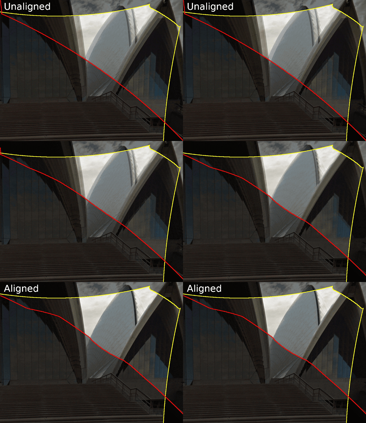
A visualization of the final warping process. Left: A section of the panorama covering 180 degrees horizontally. Notice that the overall effect of warping is intentionally quite subtle. Right: A close-up, highlighting how warping repairs the seams.
Our approach has many similarities to previously published work by Shum & Szeliski on “deghosting” panoramas. Key differences include that our approach estimates dense, smooth correspondences (rather than patch-wise, independent correspondences), and we solve a nonlinear optimization for the final warping. The result is a more well-behaved warping that is less likely to introduce new visual artifacts than the kernel-based approach.
Left: A close-up of the un-repaired panorama. Middle: Result of kernel-based interpolation. This fixes discontinuities but at the expense of strong wobbling artifacts due to the small image overlap and limited footprint of kernels. Right: Result of our global optimization.
This is important because our algorithm needs to be robust to the enormous diversity in content in Street View’s billions of panoramas. You can see how effective the algorithm is in the following examples:
Tower Bridge, London
Christ the Redeemer, Rio de Janeiro
An SUV on the streets of Seattle
This new algorithm was recently added to the Street View stitching pipeline. It is now being used to restitch existing panoramas on an ongoing basis. Keep an eye out for improved Street View near you!

Acknowledgements
Special thanks to Bryan Klingner for helping to integrate this feature with the Street View infrastructure.

Feature Visualization


Have you ever wondered what goes on inside neural networks? Feature visualization is a powerful tool for digging into neural networks and seeing how they work.

Our new article, published in Distill, does a deep exploration of feature visualization, introducing a few new tricks along the way!

Building on our work in DeepDream, and lots of work by others since, we are able to visualize what every neuron a strong vision model (GoogLeNet [1]) detects. Over the course of multiple layers, it gradually builds up abstractions: first it detects edges, then it uses those edges to detect textures, the textures to detect patterns, and the patterns to detect parts of objects….
But neurons don’t understand the world by themselves — they work together. So we also need to understand how they interact with each other. One approach is to explore interpolations between them. What images can make them both fire, to different extents?

Here we interpolate from a neuron that seems to detect artistic patterns to a neuron that seems to detect lizard eyes:
We can also let you try adding different pairs of neurons together, to explore the possibilities for yourself:
In addition to allowing you to play around with visualizations, we explore a variety of techniques for getting feature visualization to work, and let you experiment with using them.
Techniques for visualizing and understanding neural networks are becoming more powerful. We hope our article will help other researchers apply these techniques, and give people a sense of their potential. Check it out on Distill.

Acknowledgement
We're extremely grateful to our co-author, Ludwig Schurbert, who made incredible contributions to our paper and especially to the interactive visualizations.


Tangent: Source-to-Source Debuggable Derivatives


Tangent is a new, free, and open-source Python library for automatic differentiation. In contrast to existing machine learning libraries, Tangent is a source-to-source system, consuming a Python function f and emitting a new Python function that computes the gradient of f. This allows much better user visibility into gradient computations, as well as easy user-level editing and debugging of gradients. Tangent comes with many more features for debugging and designing machine learning models:
This post gives an overview of the Tangent API. It covers how to use Tangent to generate gradient code in Python that is easy to interpret, debug and modify.

Neural networks (NNs) have led to great advances in machine learning models for images, video, audio, and text. The fundamental abstraction that lets us train NNs to perform well at these tasks is a 30-year-old idea called reverse-mode automatic differentiation (also known as backpropagation), which comprises two passes through the NN. First, we run a “forward pass” to calculate the output value of each node. Then we run a “backward pass” to calculate a series of derivatives to determine how to update the weights to increase the model’s accuracy.

Training NNs, and doing research on novel architectures, requires us to compute these derivatives correctly, efficiently, and easily. We also need to be able to debug these derivatives when our model isn’t training well, or when we’re trying to build something new that we do not yet understand. Automatic differentiation, or just “autodiff,” is a technique to calculate the derivatives of computer programs that denote some mathematical function, and nearly every machine learning library implements it.

Existing libraries implement automatic differentiation by tracing a program’s execution (at runtime, like TF Eager, PyTorch and Autograd) or by building a dynamic data-flow graph and then differentiating the graph (ahead-of-time, like TensorFlow). In contrast, Tangent performs ahead-of-time autodiff on the Python source code itself, and produces Python source code as its output.

As a result, you can finally read your automatic derivative code just like the rest of your program. Tangent is useful to researchers and students who not only want to write their models in Python, but also read and debug automatically-generated derivative code without sacrificing speed and flexibility.

You can easily inspect and debug your models written in Tangent, without special tools or indirection. Tangent works on a large and growing subset of Python, provides extra autodiff features other Python ML libraries don’t have, is high-performance, and is compatible with TensorFlow and NumPy.

Automatic differentiation of Python code
How do we automatically generate derivatives of plain Python code? Math functions like tf.exp or  tf.log have derivatives, which we can compose to build the backward pass. Similarly, pieces of syntax, such as subroutines, conditionals, and loops, also have backward-pass versions. Tangent contains recipes for generating derivative code for each piece of Python syntax, along with many NumPy and TensorFlow function calls.

Tangent has a one-function API:
Here’s an animated graphic of what happens when we call tangent.grad on a Python function:
If you want to print out your derivatives, you can run:
Under the hood, tangent.grad first grabs the source code of the Python function you pass it. Tangent has a large library of recipes for the derivatives of Python syntax, as well as TensorFlow Eager functions. The function  tangent.grad then walks your code in reverse order, looks up the matching backward-pass recipe, and adds it to the end of the derivative function. This reverse-order processing gives the technique its name: reverse-mode automatic differentiation.

The function df above only works for scalar (non-array) inputs. Tangent also supports
Although we started with TensorFlow Eager support, Tangent isn’t tied to one numeric library or another—we would gladly welcome pull requests adding PyTorch or MXNet derivative recipes.

Next Steps
Tangent is open source now at github.com/google/tangent. Go check it out for download and installation instructions. Tangent is still an experiment, so expect some bugs. If you report them to us on GitHub, we will do our best to fix them quickly.

We are working to add support in Tangent for more aspects of the Python language (e.g., closures, inline function definitions, classes, more NumPy and TensorFlow functions). We also hope to add more advanced automatic differentiation and compiler functionality in the future, such as automatic trade-off between memory and compute (Griewank and Walther 2000; Gruslys et al., 2016), more aggressive optimizations, and lambda lifting.

We intend to develop Tangent together as a community. We welcome pull requests with fixes and features. Happy differentiating!

Acknowledgments
Bart van Merriënboer contributed immensely to all aspects of Tangent during his internship, and Dan Moldovan led TF Eager integration, infrastructure and benchmarking. Also, thanks to the Google Brain team for their support of this post and special thanks to Sanders Kleinfeld, Matt Johnson and Aleks Haecky for their valuable contribution for the technical aspects of the post.

AutoML for large scale image classification and object detection


A few months ago, we introduced AutoML, an approach that automates the design of machine learning models. While we found that AutoML can design small neural networks that perform on par with neural networks designed by human experts, these results were constrained to small academic datasets like CIFAR-10, and Penn Treebank. We became curious how this method would perform on larger more challenging datasets, such as ImageNet image classification and COCO object detection. Many state-of-the-art machine learning architectures have been invented by humans to tackle these datasets in academic competitions.

In Learning Transferable Architectures for Scalable Image Recognition, we apply AutoML to the ImageNet image classification and COCO object detection dataset -- two of the most respected large scale academic datasets in computer vision. These two datasets prove a great challenge for us because they are orders of magnitude larger than CIFAR-10 and Penn Treebank datasets. For instance, naively applying AutoML directly to ImageNet would require many months of training our method.

To be able to apply our method to ImageNet we have altered the AutoML approach to be more tractable to large-scale datasets:
  • We redesigned the search space so that AutoML could find the best layer which can then be stacked many times in a flexible manner to create a final network.
  • We performed architecture search on CIFAR-10 and transferred the best learned architecture to ImageNet image classification and COCO object detection.
With this method, AutoML was able to find the best layers that work well on CIFAR-10 but work well on ImageNet classification and COCO object detection. These two layers are combined to form a novel architecture, which we called “NASNet”.
Our NASNet architecture is composed of two types of layers: Normal Layer (left), and Reduction Layer (right). These two layers are designed by AutoML.

On ImageNet image classification, NASNet achieves a prediction accuracy of 82.7% on the validation set, surpassing all previous Inception models that we built [2, 3, 4]. Additionally, NASNet performs 1.2% better than all previous published results and is on par with the best unpublished result reported on arxiv.org [5]. Furthermore, NASNet may be resized to produce a family of models that achieve good accuracies while having very low computational costs. For example, a small version of NASNet achieves 74% accuracy, which is 3.1% better than equivalently-sized, state-of-the-art models for mobile platforms. The large NASNet achieves state-of-the-art accuracy while halving the computational cost of the best reported result on arxiv.org (i.e., SENet) [5].

Accuracies of NASNet and state-of-the-art, human-invented models at various model sizes on ImageNet image classification.

We also transferred the learned features from ImageNet to object detection. In our experiments, combining the features learned from ImageNet classification with the Faster-RCNN framework [6] surpassed previous published, state-of-the-art predictive performance on the COCO object detection task in both the largest as well as mobile-optimized models. Our largest model achieves 43.1% mAP which is 4% better than the previous, published state-of-the-art.

Example object detection using Faster-RCNN with NASNet.

We suspect that the image features learned by NASNet on ImageNet and COCO may be reused for many computer vision applications. Thus, we have open-sourced NASNet for inference on image classification and for object detection in the Slim and Object Detection TensorFlow repositories. We hope that the larger machine learning community will be able to build on these models to address multitudes of computer vision problems we have not yet imagined.

Special thanks to Jeff Dean, Yifeng Lu, Jonathan Huang, Vivek Rathod, Sergio Guadarrama, Chen Sun, Jonathan Shen, Vishy Tirumalashetty, Xiaoqiang Zheng, Christian Sigg and the Google Brain team for the help with the project.

References

[1] Learning Transferable Architectures for Scalable Image Recognition, Barret Zoph, Vijay Vasudevan, Jonathon Shlens, and Quoc V. Le. Arxiv, 2017.
[2] Going Deeper with Convolutions, Christian Szegedy, Wei Liu, Yangqing Jia, Pierre Sermanet, Scott Reed, Dragomir Anguelov, Dumitru Erhan, Vincent Vanhoucke, and Andrew Rabinovich. CVPR, 2015.
[3] Rethinking the inception architecture for computer vision, Christian Szegedy, Vincent Vanhoucke, Sergey Ioffe, Jonathon Shlens, and Zbigniew Wojna. CVPR, 2016.
[4] Inception-v4, Inception-ResNet and the Impact of Residual Connections on Learning, Christian Szegedy, Sergey Ioffe, Vincent Vanhoucke, and Alex Alemi. AAAI, 2017.
[5] Squeeze-and-Excitation Networks, Jie Hu, Li Shen and Gang Sun. Arxiv, 2017.
[6] Faster R-CNN: Towards Real-Time Object Detection with Region Proposal Networks, Shaoqing Ren, Kaiming He, Ross Girshick and Jian Sun. NIPS, 2015.


Latest Innovations in TensorFlow Serving


Since initially open-sourcing TensorFlow Serving in February 2016, we’ve made some major enhancements. Let’s take a look back at where we started, review our progress, and share where we are headed next.

Before TensorFlow Serving, users of TensorFlow inside Google had to create their own serving system from scratch. Although serving might appear easy at first, one-off serving solutions quickly grow in complexity. Machine Learning (ML) serving systems need to support model versioning (for model updates with a rollback option) and multiple models (for experimentation via A/B testing), while ensuring that concurrent models achieve high throughput on hardware accelerators (GPUs and TPUs) with low latency. So we set out to create a single, general TensorFlow Serving software stack.

We decided to make it open-sourceable from the get-go, and development started in September 2015. Within a few months, we created the initial end-to-end working system and our open-source release in February 2016.

Over the past year and half, with the help of our users and partners inside and outside our company, TensorFlow Serving has advanced performance, best practices, and standards:
  • Out-of-the-box optimized serving and customizability: We now offer a pre-built canonical serving binary, optimized for modern CPUs with AVX, so developers don't need to assemble their own binary from our libraries unless they have exotic needs. At the same time, we added a registry-based framework, allowing our libraries to be used for custom (or even non-TensorFlow) serving scenarios.
  • Multi-model serving: Going from one model to multiple concurrently-served models presents several performance obstacles. We serve multiple models smoothly by (1) loading in isolated thread pools to avoid incurring latency spikes on other models taking traffic; (2) accelerating initial loading of all models in parallel upon server start-up; (3) multi-model batch interleaving to multiplex hardware accelerators (GPUs/TPUs).
  • Standardized model format: We added SavedModel to TensorFlow 1.0, giving the community a single standard model format that works across training and serving.
  • Easy-to-use inference APIs: We released easy-to-use APIs for common inference tasks (classification, regression) that we know work for a wide swathe of our applications. To support more advanced use-cases we support a lower-level tensor-based API (predict) and a new multi-inference API that enables multi-task modeling.
All of our work has been informed by close collaborations with: (a) Google’s ML SRE team, which helps ensure we are robust and meet internal SLAs; (b) other Google machine learning infrastructure teams including ads serving and TFX; (c) application teams such as Google Play; (d) our partners at the UC Berkeley RISE Lab, who explore complementary research problems with the Clipper serving system; (e) our open-source user base and contributors.

TensorFlow Serving is currently handling tens of millions of inferences per second for 1100+ of our own projects including Google’s Cloud ML Prediction. Our core serving code is available to all via our open-source releases.

Looking forward, our work is far from done and we are exploring several avenues of innovation. Today we are excited to share early progress in two experimental areas:
  • Granular batching: A key technique we employ to achieve high throughput on specialized hardware (GPUs and TPUs) is "batching": processing multiple examples jointly for efficiency. We are developing technology and best practices to improve batching to: (a) enable batching to target just the GPU/TPU portion of the computation, for maximum efficiency; (b) enable batching within recursive neural networks, used to process sequence data e.g. text and event sequences. We are experimenting with batching arbitrary sub-graphs using the Batch/Unbatch op pair.
  • Distributed model serving: We are looking at model sharding techniques as a means of handling models that are too large to fit on one server node or sharing sub-models in a memory-efficient way. We recently launched a 1TB+ model in production with good results, and hope to open-source this capability soon.
Thanks again to all of our users and partners who have contributed feedback, code and ideas. Join the project at: github.com/tensorflow/serving.

Eager Execution: An imperative, define-by-run interface to TensorFlow


Today, we introduce eager execution for TensorFlow. Eager execution is an imperative, define-by-run interface where operations are executed immediately as they are called from Python. This makes it easier to get started with TensorFlow, and can make research and development more intuitive.

The benefits of eager execution include:
  • Fast debugging with immediate run-time errors and integration with Python tools
  • Support for dynamic models using easy-to-use Python control flow
  • Strong support for custom and higher-order gradients
  • Almost all of the available TensorFlow operations
Eager execution is available now as an experimental feature, so we're looking for feedback from the community to guide our direction.

To understand this all better, let's look at some code. This gets pretty technical; familiarity with TensorFlow will help.

Using Eager Execution

When you enable eager execution, operations execute immediately and return their values to Python without requiring a Session.run(). For example, to multiply two matrices together, we write this:
import tensorflow as tf
import tensorflow.contrib.eager as tfe

tfe.enable_eager_execution()

x = [[2.]]
m = tf.matmul(x, x)
It’s straightforward to inspect intermediate results with print or the Python debugger.
print(m)
# The 1x1 matrix [[4.]]
Dynamic models can be built with Python flow control. Here's an example of the Collatz conjecture using TensorFlow’s arithmetic operations:
a = tf.constant(12)
counter = 0
while not tf.equal(a, 1):
if tf.equal(a % 2, 0):
a = a / 2
else:
a = 3 * a + 1
print(a)
Here, the use of the tf.constant(12) Tensor object will promote all math operations to tensor operations, and as such all return values with be tensors.

Gradients

Most TensorFlow users are interested in automatic differentiation. Because different operations can occur during each call, we record all forward operations to a tape, which is then played backwards when computing gradients. After we've computed the gradients, we discard the tape.

If you’re familiar with the autograd package, the API is very similar. For example:
def square(x):
return tf.multiply(x, x)

grad = tfe.gradients_function(square)

print(square(3.)) # [9.]
print(grad(3.)) # [6.]
The gradients_function call takes a Python function square() as an argument and returns a Python callable that computes the partial derivatives of square() with respect to its inputs. So, to get the derivative of square() at 3.0, invoke grad(3.0), which is 6.

The same gradients_function call can be used to get the second derivative of square:
gradgrad = tfe.gradients_function(lambda x: grad(x)[0])

print(gradgrad(3.)) # [2.]
As we noted, control flow can cause different operations to run, such as in this example.
def abs(x):
return x if x > 0. else -x

grad = tfe.gradients_function(abs)

print(grad(2.0)) # [1.]
print(grad(-2.0)) # [-1.]

Custom Gradients

Users may want to define custom gradients for an operation, or for a function. This may be useful for multiple reasons, including providing a more efficient or more numerically stable gradient for a sequence of operations.

Here is an example that illustrates the use of custom gradients. Let's start by looking at the function log(1 + ex), which commonly occurs in the computation of cross entropy and log likelihoods.
def log1pexp(x):
return tf.log(1 + tf.exp(x))
grad_log1pexp = tfe.gradients_function(log1pexp)

# The gradient computation works fine at x = 0.
print(grad_log1pexp(0.))
# [0.5]
# However it returns a `nan` at x = 100 due to numerical instability.
print(grad_log1pexp(100.))
# [nan]
We can use a custom gradient for the above function that analytically simplifies the gradient expression. Notice how the gradient function implementation below reuses an expression (tf.exp(x)) that was computed during the forward pass, making the gradient computation more efficient by avoiding redundant computation.
@tfe.custom_gradient
def log1pexp(x):
e = tf.exp(x)
def grad(dy):
return dy * (1 - 1 / (1 + e))
return tf.log(1 + e), grad
grad_log1pexp = tfe.gradients_function(log1pexp)

# Gradient at x = 0 works as before.
print(grad_log1pexp(0.))
# [0.5]
# And now gradient computation at x=100 works as well.
print(grad_log1pexp(100.))
# [1.0]

Building models

Models can be organized in classes. Here's a model class that creates a (simple) two layer network that can classify the standard MNIST handwritten digits.
class MNISTModel(tfe.Network):
def __init__(self):
super(MNISTModel, self).__init__()
self.layer1 = self.track_layer(tf.layers.Dense(units=10))
self.layer2 = self.track_layer(tf.layers.Dense(units=10))
def call(self, input):
"""Actually runs the model."""
result = self.layer1(input)
result = self.layer2(result)
return result
We recommend using the classes (not the functions) in tf.layers since they create and contain model parameters (variables). Variable lifetimes are tied to the lifetime of the layer objects, so be sure to keep track of them.

Why are we using tfe.Network? A Network is a container for layers and is a tf.layer.Layer itself, allowing Network objects to be embedded in other Network objects. It also contains utilities to assist with inspection, saving, and restoring.

Even without training the model, we can imperatively call it and inspect the output:
# Let's make up a blank input image
model = MNISTModel()
batch = tf.zeros([1, 1, 784])
print(batch.shape)
# (1, 1, 784)
result = model(batch)
print(result)
# tf.Tensor([[[ 0. 0., ...., 0.]]], shape=(1, 1, 10), dtype=float32)
Note that we do not need any placeholders or sessions. The first time we pass in the input, the sizes of the layers’ parameters are set.

To train any model, we define a loss function to optimize, calculate gradients, and use an optimizer to update the variables. First, here's a loss function:
def loss_function(model, x, y):
y_ = model(x)
return tf.nn.softmax_cross_entropy_with_logits(labels=y, logits=y_)
And then, our training loop:
optimizer = tf.train.GradientDescentOptimizer(learning_rate=0.001)
for (x, y) in tfe.Iterator(dataset):
grads = tfe.implicit_gradients(loss_function)(model, x, y)
optimizer.apply_gradients(grads)
implicit_gradients() calculates the derivatives of loss_function with respect to all the TensorFlow variables used during its computation.

We can move computation to a GPU the same way we’ve always done with TensorFlow:
with tf.device("/gpu:0"):
for (x, y) in tfe.Iterator(dataset):
optimizer.minimize(lambda: loss_function(model, x, y))
(Note: We're shortcutting storing our loss and directly calling the optimizer.minimize, but you could also use the apply_gradients() method above; they are equivalent.)

Using Eager with Graphs

Eager execution makes development and debugging far more interactive, but TensorFlow graphs have a lot of advantages with respect to distributed training, performance optimizations, and production deployment.

The same code that executes operations when eager execution is enabled will construct a graph describing the computation when it is not. To convert your models to graphs, simply run the same code in a new Python session where eager execution hasn’t been enabled, as seen, for example, in the MNIST example. The value of model variables can be saved and restored from checkpoints, allowing us to move between eager (imperative) and graph (declarative) programming easily. With this, models developed with eager execution enabled can be easily exported for production deployment.

In the near future, we will provide utilities to selectively convert portions of your model to graphs. In this way, you can fuse parts of your computation (such as internals of a custom RNN cell) for high-performance, but also keep the flexibility and readability of eager execution.

How does my code change?

Using eager execution should be intuitive to current TensorFlow users. There are only a handful of eager-specific APIs; most of the existing APIs and operations work with eager enabled. Some notes to keep in mind:
  • As with TensorFlow generally, we recommend that if you have not yet switched from queues to using tf.data for input processing, you should. It's easier to use and usually faster. For help, see this blog post and the documentation page.
  • Use object-oriented layers, like tf.layer.Conv2D() or Keras layers; these have explicit storage for variables.
  • For most models, you can write code so that it will work the same for both eager execution and graph construction. There are some exceptions, such as dynamic models that use Python control flow to alter the computation based on inputs.
  • Once you invoke tfe.enable_eager_execution(), it cannot be turned off. To get graph behavior, start a new Python session.

Getting started and the future

This is still a preview release, so you may hit some rough edges. To get started today:
There's a lot more to talk about with eager execution and we're excited… or, rather, we're eager for you to try it today! Feedback is absolutely welcome.

Closing the Simulation-to-Reality Gap for Deep Robotic Learning


Each of us can learn remarkably complex skills that far exceed the proficiency and robustness of even the most sophisticated robots, when it comes to basic sensorimotor skills like grasping. However, we also draw on a lifetime of experience, learning over the course of multiple years how to interact with the world around us. Requiring such a lifetime of experience for a learning-based robot system is quite burdensome: the robot would need to operate continuously, autonomously, and initially at a low level of proficiency before it can become useful. Fortunately, robots have a powerful tool at their disposal: simulation.

Simulating many years of robotic interaction is quite feasible with modern parallel computing, physics simulation, and rendering technology. Moreover, the resulting data comes with automatically-generated annotations, which is particularly important for tasks where success is hard to infer automatically. The challenge with simulated training is that even the best available simulators do not perfectly capture reality. Models trained purely on synthetic data fail to generalize to the real world, as there is a discrepancy between simulated and real environments, in terms of both visual and physical properties. In fact, the more we increase the fidelity of our simulations, the more effort we have to expend in order to build them, both in terms of implementing complex physical phenomena and in terms of creating the content (e.g., objects, backgrounds) to populate these simulations. This difficulty is compounded by the fact that powerful optimization methods based on deep learning are exceptionally proficient at exploiting simulator flaws: the more powerful the machine learning algorithm, the more likely it is to discover how to "cheat" the simulator to succeed in ways that are infeasible in the real world. The question then becomes: how can a robot utilize simulation to enable it to perform useful tasks in the real world?

The difficulty of transferring simulated experience into the real world is often called the "reality gap." The reality gap is a subtle but important discrepancy between reality and simulation that prevents simulated robotic experience from directly enabling effective real-world performance. Visual perception often constitutes the widest part of the reality gap: while simulated images continue to improve in fidelity, the peculiar and pathological regularities of synthetic pictures, and the wide, unpredictable diversity of real-world images, makes bridging the reality gap particularly difficult when the robot must use vision to perceive the world, as is the case for example in many manipulation tasks. Recent advances in closing the reality gap with deep learning in computer vision for tasks such as object classification and pose estimation provide promising solutions.  For example,  Shrivastava et al. and Bousmalis et al. explored pixel-level domain adaptation. Ganin et al. and Bousmalis and Trigeorgis et al. focus on feature-level domain adaptation. These advances required a rethinking of the approaches used to solve the simulation-to-reality domain shift problem for robotic manipulation as well. Although a number of recent works have sought to address the reality gap in robotics, through techniques such as machine learning-based domain adaptation (Tzeng et al.) and randomization of simulated environments (Sadeghi and Levine), effective transfer in robotic manipulation has been limited to relatively simple tasks, such as grasping rectangular, brightly-colored objects (Tobin et al. and James et al.) and free-space motion (Christiano et al.).  In this post, we describe how learning in simulation, in our case PyBullet, and using domain adaptation methods such as machine learning methods that deal with the simulation-to-reality domain shift, can accelerate learning of robotic grasping in the real world. This approach can enable real robots to grasp a large of variety physical objects, unseen during training, with a high degree of proficiency.

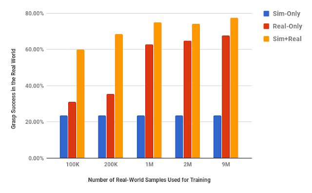
The performance effect of using 8 million simulated samples of procedural objects with no randomization and various amounts of real data.

Before we consider introducing simulated experience, what does it take for our robots to learn to reliably grasp such not-before-seen objects with only real-world experience? In a previous post, we discussed how the Google Brain team and X’s robotics teams teach robots how to grasp a variety of ordinary objects by just using images from a single monocular camera. It takes tens to hundreds of thousands of grasp attempts, the equivalent of thousands of robot-hours of real-world experience. Although distributing the learning across multiple robots expedites this, the realities of real-world data collection, including maintenance and wear-and-tear, mean that these kinds of data collection efforts still take a significant amount of real time. As mentioned above, an appealing alternative is to use off-the-shelf simulators and learn basic sensorimotor skills like grasping in a virtual environment. Training a robot how to grasp in simulation can be parallelized easily over any number of machines, and can provide large amounts of experience in dramatically less time (e.g., hours rather than months) and at a fraction of the cost.


If the goal is to bridge the reality gap for vision-based robotic manipulation, we must answer a few critical questions. First, how do we design simulation so that simulated experience appears realistic to a neural network? And second, how should we integrate simulated and real experience in a way that maximizes transfer to the real world? We studied these questions in the context of a particularly challenging and important robotic manipulation task: vision-based grasping of diverse objects. We extensively evaluated the effect of various simulation design decisions in combination with various techniques for integrating simulated and real experience for maximal performance.
The setup we used for collecting the simulated and real-world datasets.

Images used during training of simulated grasping experience with procedurally generated objects (left) and of real-world experience with a varied collection of everyday physical objects (right). In both cases, we see pairs of image inputs with and without the robot arm present.
When it comes to simulation, there are a number of choices we have to make: the type of objects to use for simulated grasping, whether to use appearance and/or dynamics randomization, and whether to extract any additional information from the simulator that could aid adaptation to the real world. The types of objects we use in simulation is a particularly important one, and there are a number of choices. A question that comes naturally is: how realistic do the objects used in simulation need to be? Using randomly generated procedural objects is the most desirable choice, because these objects are generated effortlessly on demand, and are easy to parameterize if we change the requirements of the task. However, they are not realistic and one could imagine they might not be useful for transferring the experience of grasping them to the real world. Using realistic 3D object models from a publicly available model library, such as the widely used ShapeNet, is another choice, which however restricts our findings to be related to the characteristics of the specific models we are using. In this work, we compared the effect of using procedurally-generated and realistic objects from the ShapeNet model repository, and found that simply using random objects generated programmatically was not just sufficient for efficient experience transfer from simulation to reality, but also generalized better to the real world than using ShapeNet ones.

Some of the procedurally-generated objects used in simulation.

Some of the ShapeNet objects used in simulation.

Some of the physical objects used to collect real grasping experience.
Another decision about our simulated environment has to do with the randomization of the simulation. Simulation randomization has shown promise in providing generalization to real-world environments in previous work. We further evaluate randomization as a way to provide generalization by separately evaluating the effect of using appearance randomization (randomly changing textures of different visual components of the virtual environment), and dynamics randomization (randomly changing object mass, and friction properties). For our task, visual randomization had a positive effect when we did not use domain adaptation methods to aid with generalization, and had no effect when we included domain adaptation. Using dynamics randomization did not show a significant improvement for this particular task, however it is possible that dynamics randomization might be more relevant in other tasks. These results suggest that, although randomization can be an important part of simulation-to-real-world transfer, the inclusion of effective domain adaptation can have a substantially more pronounced impact for vision-based manipulation tasks.

Appearance randomization in simulation.
Finally, the information we choose to extract and use for our domain adaptation methods has a significant impact on performance. In one of our proposed methods, we utilize the extracted semantic map of the simulated image, ie the description of each pixel in the simulated image, and use it to ground our proposed domain adaptation approach to produce semantically-meaningful realistic samples, as we discuss below.

Our main proposed approach to integrating simulated and real experience, which we call GraspGAN, takes as input synthetic images generated by a simulator, along with their semantic maps, and produces adapted images that look similar to real-world ones. This is possible with adversarial training, a powerful idea proposed by Goodfellow et al. In our framework, a convolutional neural network, the generator, takes as input synthetic images and generates images that another neural network, the discriminator, cannot distinguish from actual real images. The generator and discriminator networks are trained simultaneously and improve together, resulting in a generator that can produce images that are both realistic and useful for learning a grasping model that will generalize to the real world. One way to make sure that these images are useful is the use of the semantic maps of the synthetic images to ground the generator. By using the prediction of these masks as an auxiliary task, the generator is encouraged to produce meaningful adapted images that correspond to the original label attributed to the simulated experience. We train a deep vision-based grasping model with both visually-adapted simulated and real images, and attempt to account for the domain shift further by using a feature-level domain adaptation technique which helps produce a domain-invariant model. See below the GraspGAN adapting simulated images to realistic ones and a semantic map it infers.


By using synthetic data and domain adaptation we are able to reduce the number of real-world samples required to achieve a given level of performance by up to 50 times, using only randomly generated objects in simulation. This means that we have no prior information about the objects in the real world, other than pre-specified size limits for the graspable objects. We have shown that we are able to increase performance with various amounts of real-world data, and also that by using only unlabeled real-world data and our GraspGAN methodology, we obtain real-world grasping performance without any real-world labels that is similar to that achieved with hundreds of thousands of labeled real-world samples. This suggests that, instead of collecting labeled experience, it may be sufficient in the future to simply record raw unlabeled images, use them to train a GraspGAN model, and then learn the skills themselves in simulation.

Although this work has not addressed all the issues around closing the reality gap, we believe that our results show that using simulation and domain adaptation to integrate simulated and real robotic experience is an attractive choice for training robots. Most importantly, we have extensively evaluated the performance gains for different available amounts of labeled real-world samples, and for the different design choices for both the simulator and the domain adaptation methods used. This evaluation can hopefully serve as a guide for practitioners to use for their own design decisions and for weighing the advantages and disadvantages of incorporating such an approach in their experimental design.

This research was conducted by K. Bousmalis, A. Irpan, P. Wohlhart, Y. Bai, M, Kelcey, M. Kalakrishnan, L. Downs, J. Ibarz, P. Pastor, K. Konolige, S. Levine, V. Vanhoucke, with special thanks to colleagues at Google Research and X who've contributed their expertise and time to this research. An early preprint is available on arXiv.

The collection of procedurally-generated objects we used in simulation was made publicly available here by Laura Downs.


Announcing OpenFermion: The Open Source Chemistry Package for Quantum Computers


“The underlying physical laws necessary for the mathematical theory of a large part of physics and the whole of chemistry are thus completely known, and the difficulty is only that the exact application of these laws leads to equations much too complicated to be soluble.”
-Paul Dirac, Quantum Mechanics of Many-Electron Systems (1929)

In this passage, physicist Paul Dirac laments that while quantum mechanics accurately models all of chemistry, exactly simulating the associated equations appears intractably complicated. Not until 1982 would Richard Feynman suggest that instead of surrendering to the complexity of quantum mechanics, we might harness it as a computational resource. Hence, the original motivation for quantum computing: by operating a computer according to the laws of quantum mechanics, one could efficiently unravel exact simulations of nature. Such simulations could lead to breakthroughs in areas such as photovoltaics, batteries, new materials, pharmaceuticals and superconductivity. And while we do not yet have a quantum computer large enough to solve classically intractable problems in these areas, rapid progress is being made. Last year, Google published this paper detailing the first quantum computation of a molecule using a superconducting qubit quantum computer. Building on that work, the quantum computing group at IBM scaled the experiment to larger molecules, which made the cover of Nature last month.

Today, we announce the release of OpenFermion, the first open source platform for translating problems in chemistry and materials science into quantum circuits that can be executed on existing platforms. OpenFermion is a library for simulating the systems of interacting electrons (fermions) which give rise to the properties of matter. Prior to OpenFermion, quantum algorithm developers would need to learn a significant amount of chemistry and write a large amount of code hacking apart other codes to put together even the most basic quantum simulations. While the project began at Google, collaborators at ETH Zurich, Lawrence Berkeley National Labs, University of Michigan, Harvard University, Oxford University, Dartmouth University, Rigetti Computing and NASA all contributed to alpha releases. You can learn more details about this release in our paper, OpenFermion: The Electronic Structure Package for Quantum Computers.

One way to think of OpenFermion is as a tool for generating and compiling physics equations which describe chemical and material systems into representations which can be interpreted by a quantum computer1. The most effective quantum algorithms for these problems build upon and extend the power of classical quantum chemistry packages used and developed by research chemists across government, industry and academia. Accordingly, we are also releasing OpenFermion-Psi4 and OpenFermion-PySCF which are plugins for using OpenFermion in conjunction with the classical electronic structure packages Psi4 and PySCF.

The core OpenFermion library is designed in a quantum programming framework agnostic way to ensure compatibility with various platforms being developed by the community. This allows OpenFermion to support external packages which compile quantum assembly language specifications for diverse hardware platforms. We hope this decision will help establish OpenFermion as a community standard for putting quantum chemistry on quantum computers. To see how OpenFermion is used with diverse quantum programming frameworks, take a look at OpenFermion-ProjectQ and Forest-OpenFermion - plugins which link OpenFermion to the externally developed circuit simulation and compilation platforms known as ProjectQ and Forest.

The following workflow describes how a quantum chemist might use OpenFermion in order to simulate the energy surface of a molecule (for instance, by preparing the sort of quantum computation we described in our past blog post):
  1. The researcher initializes an OpenFermion calculation with specification of:
    • An input file specifying the coordinates of the nuclei in the molecule.
    • The basis set (e.g. cc-pVTZ) that should be used to discretize the molecule.
    • The charge and spin multiplicity (if known) of the system.
  1. The researcher uses the OpenFermion-Psi4 plugin or the OpenFermion-PySCF plugin to perform scalable classical computations which are used to optimally stage the quantum computation. For instance, one might perform a classical Hartree-Fock calculation to choose a good initial state for the quantum simulation.
  2. The researcher then specifies which electrons are most interesting to study on a quantum computer (known as an active space) and asks OpenFermion to map the equations for those electrons to a representation suitable for quantum bits, using one of the available procedures in OpenFermion, e.g. the Bravyi-Kitaev transformation.
  3. The researcher selects a quantum algorithm to solve for the properties of interest and uses a quantum compilation framework such as OpenFermion-ProjectQ to output the quantum circuit in assembly language which can be run on a quantum computer. If the researcher has access to a quantum computer, they then execute the experiment.
A few examples of what one might do with OpenFermion are demonstrated in ipython notebooks here, here and here. While quantum simulation is widely recognized as one of the most important applications of quantum computing in the near term, very few quantum computer scientists know quantum chemistry and even fewer chemists know quantum computing. Our hope is that OpenFermion will help to close the gap between these communities and bring the power of quantum computing to chemists and material scientists. If you’re interested, please checkout our GitHub repository - pull requests welcome!


1 If we may be allowed one sentence for the experts: the primary function of OpenFermion is to encode the electronic structure problem in second quantization defined by various basis sets and active spaces and then to transform those operators into spin Hamiltonians using various isomorphisms between qubit and fermion algebras.

Announcing AVA: A Finely Labeled Video Dataset for Human Action Understanding


Teaching machines to understand human actions in videos is a fundamental research problem in Computer Vision, essential to applications such as personal video search and discovery, sports analysis, and gesture interfaces. Despite exciting breakthroughs made over the past years in classifying and finding objects in images, recognizing human actions still remains a big challenge. This is due to the fact that actions are, by nature, less well-defined than objects in videos, making it difficult to construct a finely labeled action video dataset. And while many benchmarking datasets, e.g., UCF101, ActivityNet and DeepMind’s Kinetics, adopt the labeling scheme of image classification and assign one label to each video or video clip in the dataset, no dataset exists for complex scenes containing multiple people who could be performing different actions.

In order to facilitate further research into human action recognition, we have released AVA, coined from “atomic visual actions”, a new dataset that provides multiple action labels for each person in extended video sequences. AVA consists of URLs for publicly available videos from YouTube, annotated with a set of 80 atomic actions (e.g. “walk”, “kick (an object)”, “shake hands”) that are spatial-temporally localized, resulting in 57.6k video segments, 96k labeled humans performing actions, and a total of 210k action labels. You can browse the website to explore the dataset and download annotations, and read our arXiv paper that describes the design and development of the dataset.

Compared with other action datasets, AVA possesses the following key characteristics:
  • Person-centric annotation. Each action label is associated with a person rather than a video or clip. Hence, we are able to assign different labels to multiple people performing different actions in the same scene, which is quite common.
  • Atomic visual actions. We limit our action labels to fine temporal scales (3 seconds), where actions are physical in nature and have clear visual signatures.
  • Realistic video material. We use movies as the source of AVA, drawing from a variety of genres and countries of origin. As a result, a wide range of human behaviors appear in the data.
Examples of 3-second video segments (from Video Source) with their bounding box annotations in the middle frame of each segment. (For clarity, only one bounding box is shown for each example.)

To create AVA, we first collected a diverse set of long form content from YouTube, focusing on the “film” and “television” categories, featuring professional actors of many different nationalities. We analyzed a 15 minute clip from each video, and uniformly partitioned it into 300 non-overlapping 3-second segments. The sampling strategy preserved sequences of actions in a coherent temporal context.

Next, we manually labeled all bounding boxes of persons in the middle frame of each 3-second segment. For each person in the bounding box, annotators selected a variable number of labels from a pre-defined atomic action vocabulary (with 80 classes) that describe the person’s actions within the segment. These actions were divided into three groups: pose/movement actions, person-object interactions, and person-person interactions. Because we exhaustively labeled all people performing all actions, the frequencies of AVA’s labels followed a long-tail distribution, as summarized below.
Distribution of AVA’s atomic action labels. Labels displayed in the x-axis are only a partial set of our vocabulary.

The unique design of AVA allows us to derive some interesting statistics that are not available in other existing datasets. For example, given the large number of persons with at least two labels, we can measure the co-occurrence patterns of action labels. The figure below shows the top co-occurring action pairs in AVA with their co-occurrence scores. We confirm expected patterns such as people frequently play instruments while singing, lift a person while playing with kids, and hug while kissing.
Top co-occurring action pairs in AVA.

To evaluate the effectiveness of human action recognition systems on the AVA dataset, we implemented an existing baseline deep learning model that obtains highly competitive performance on the much smaller JHMDB dataset. Due to challenging variations in zoom, background clutter, cinematography, and appearance variation, this model achieves a relatively modest performance when correctly identifying actions on AVA (18.4% mAP). This suggests that AVA will be a useful testbed for developing and evaluating new action recognition architectures and algorithms for years to come.

We hope that the release of AVA will help improve the development of human action recognition systems, and provide opportunities to model complex activities based on labels with fine spatio-temporal granularity at the level of individual person’s actions. We will continue to expand and improve AVA, and are eager to hear feedback from the community to help us guide future directions. Please join the AVA users mailing list to receive dataset updates as well as to send us emails for feedback.

Acknowledgements
The core team behind AVA includes Chunhui Gu, Chen Sun, David Ross, Caroline Pantofaru, Yeqing Li, Sudheendra Vijayanarasimhan, George Toderici, Susanna Ricco, Rahul Sukthankar, Cordelia Schmid, and Jitendra Malik. We thank many Google colleagues and annotators for their dedicated support on this project.