Author Archives: Research Blog

TFGAN: A Lightweight Library for Generative Adversarial Networks


(Crossposted on the Google Open Source Blog)

Training a neural network usually involves defining a loss function, which tells the network how close or far it is from its objective. For example, image classification networks are often given a loss function that penalizes them for giving wrong classifications; a network that mislabels a dog picture as a cat will get a high loss. However, not all problems have easily-defined loss functions, especially if they involve human perception, such as image compression or text-to-speech systems. Generative Adversarial Networks (GANs), a machine learning technique that has led to improvements in a wide range of applications including generating images from text, superresolution, and helping robots learn to grasp, offer a solution. However, GANs introduce new theoretical and software engineering challenges, and it can be difficult to keep up with the rapid pace of GAN research.
A video of a generator improving over time. It begins by producing random noise, and eventually learns to generate MNIST digits.
In order to make GANs easier to experiment with, we’ve open sourced TFGAN, a lightweight library designed to make it easy to train and evaluate GANs. It provides the infrastructure to easily train a GAN, provides well-tested loss and evaluation metrics, and gives easy-to-use examples that highlight the expressiveness and flexibility of TFGAN. We’ve also released a tutorial that includes a high-level API to quickly get a model trained on your data.
This demonstrates the effect of an adversarial loss on image compression. The top row shows image patches from the ImageNet dataset. The middle row shows the results of compressing and uncompressing an image through an image compression neural network trained on a traditional loss. The bottom row shows the results from a network trained with a traditional loss and an adversarial loss. The GAN-loss images are sharper and more detailed, even if they are less like the original.
TFGAN supports experiments in a few important ways. It provides simple function calls that cover the majority of GAN use-cases so you can get a model running on your data in just a few lines of code, but is built in a modular way to cover more exotic GAN designs as well. You can just use the modules you want — loss, evaluation, features, training, etc. are all independent. TFGAN’s lightweight design also means you can use it alongside other frameworks, or with native TensorFlow code. GAN models written using TFGAN will easily benefit from future infrastructure improvements, and you can select from a large number of already-implemented losses and features without having to rewrite your own. Lastly, the code is well-tested, so you don’t have to worry about numerical or statistical mistakes that are easily made with GAN libraries.
Most neural text-to-speech (TTS) systems produce over-smoothed spectrograms. When applied to the Tacotron TTS system, a GAN can recreate some of the realistic-texture, which reduces artifacts in the resulting audio.
When you use TFGAN, you’ll be using the same infrastructure that many Google researchers use, and you’ll have access to the cutting-edge improvements that we develop with the library. Anyone can contribute to the github repositories, which we hope will facilitate code-sharing among ML researchers and users.

Introducing Appsperiments: Exploring the Potentials of Mobile Photography


Each of the world's approximately two billion smartphone owners is carrying a camera capable of capturing photos and video of a tonal richness and quality unimaginable even five years ago. Until recently, those cameras behaved mostly as optical sensors, capturing light and operating on the resulting image's pixels. The next generation of cameras, however, will have the capability to blend hardware and computer vision algorithms that operate as well on an image's semantic content, enabling radically new creative mobile photo and video applications.

Today, we're launching the first installment of a series of photography appsperiments: usable and useful mobile photography experiences built on experimental technology. Our "appsperimental" approach was inspired in part by Motion Stills, an app developed by researchers at Google that converts short videos into cinemagraphs and time lapses using experimental stabilization and rendering technologies. Our appsperiments replicate this approach by building on other technologies in development at Google. They rely on object recognition, person segmentation, stylization algorithms, efficient image encoding and decoding technologies, and perhaps most importantly, fun!

Storyboard
Storyboard (Android) transforms your videos into single-page comic layouts, entirely on device. Simply shoot a video and load it in Storyboard. The app automatically selects interesting video frames, lays them out, and applies one of six visual styles. Save the comic or pull down to refresh and instantly produce a new one. There are approximately 1.6 trillion different possibilities!

Selfissimo!
Selfissimo! (iOS, Android) is an automated selfie photographer that snaps a stylish black and white photo each time you pose. Tap the screen to start a photoshoot. The app encourages you to pose and captures a photo whenever you stop moving. Tap the screen to end the session and review the resulting contact sheet, saving individual images or the entire shoot.

Scrubbies
Scrubbies (iOS) lets you easily manipulate the speed and direction of video playback to produce delightful video loops that highlight actions, capture funny faces, and replay moments. Shoot a video in the app and then remix it by scratching it like a DJ. Scrubbing with one finger plays the video. Scrubbing with two fingers captures the playback so you can save or share it.

Try them out and tell us what you think using the in-app feedback links. The feedback and ideas we get from the new and creative ways people use our appsperiments will help guide some of the technology we develop next.

Acknowledgements
These appsperiments represent a collaboration across many teams at Google. We would like to thank the core contributors Andy Dahley, Ashley Ma, Dexter Allen, Ignacio Garcia Dorado, Madison Le, Mark Bowers, Pascal Getreuer, Robin Debreuil, Suhong Jin, and William Lindmeier. We also wish to give special thanks to Buck Bourdon, Hossein Talebi, Kanstantsin Sokal, Karthik Raveendran, Matthias Grundmann, Peyman Milanfar, Suril Shah, Tomas Izo, Tyler Mullen, and Zheng Sun.

Introducing a New Foveation Pipeline for Virtual/Mixed Reality


Virtual Reality (VR) and Mixed Reality (MR) offer a novel way to immerse people into new and compelling experiences, from gaming to professional training. However, current VR/MR technologies present a fundamental challenge: to present images at the extremely high resolution required for immersion places enormous demands on the rendering engine and transmission process. Headsets often have insufficient display resolution, which can limit the field of view, worsening the experience. But, to drive a higher resolution headset, the traditional rendering pipeline requires significant processing power that even high-end mobile processors cannot achieve. As research continues to deliver promising new techniques to increase display resolution, the challenges of driving those displays will continue to grow.

In order to further improve the visual experience in VR and MR, we introduce a pipeline that takes advantage of the characteristics of human visual perception to enable a amazing visual experience at low compute and power cost. The pipeline proposed in this article considers the full system dependency including the rendering engine, memory bandwidth and capability of display module itself. We determined that the current limitation is not just in the content creation, but it also may be in transmitting data, handling latency and enabling interaction with real objects (mixed reality applications). The pipeline consists of 1. Foveated Rendering with a focus on reducing of compute per pixel. 2. Foveated Image Processing with a focus on the reduction of visual artifacts and 3. Foveated Transmission with a focus on bits per pixel transmitted.

Foveated Rendering
In the human visual system, the fovea centralis allows us to see at high-fidelity in the center of our vision, allowing our brain to pay less attention to things in our peripheral vision. Foveated rendering takes advantage of this characteristic to improve the performance of the rendering engine by reducing the spatial or bit-depth resolution of objects in our peripheral vision. To make this work, the location of the High Acuity (HA) region needs to be updated with eye-tracking to align with eye saccades, which preserves the perception of a constant high-resolution across the field of view. In contrast, systems with no eye-tracking may need to render a much larger HA region.
The left image is rendered at full resolution. The right image uses two layers of foveation — one rendered at high resolution (inside the yellow region) and one at lower resolution (outside).
A traditional foveation technique may divide a frame buffer into multiple spatial resolution regions. Aliasing introduced by rendering to lower spatial resolution may cause perceptible temporal artifacts when there is motion in the content due to head motion or animation. Below we show an example of temporal artifacts introduced by head rotation.
A smooth full rendering (image on the left). The image on the right shows temporal artifacts introduced by motion in foveated region.
In the following sections, we present two different methods we use aimed at reducing these artifacts: Phase-Aligned Foveated Rendering and Conformal Foveated Rendering. Each of these methods provide different benefits for visual quality during rendering and are useful under different conditions.

Phase-Aligned Rendering
Aliasing occurs in the Low-Acuity (LA) region during foveated rendering due to the subsampling of rendered content. In traditional foveated rendering discussed above, these aliasing artifacts flicker from frame to frame, since the display pixel grid moves across the virtual scene as the user moves their head. The motion of these pixels relative to the scene cause any existing aliasing artifacts to flicker, which is highly perceptible to the user, even in the periphery.

In Phase-Aligned rendering, we force the LA region frustums to be aligned rotationally to the world (e.g. always facing north, east, south, etc.), not the current frame's head-rotation. The aliasing artifacts are mostly invariant to head pose and therefore much less detectable. After upsampling, these regions are then reprojected onto the final display screen to compensate for the user's head rotation, which reduces temporal flicker. As with traditional foveation, we render the high-acuity region in a separate pass, and overlay it onto the merged image at the location of the fovea. The figure below compares traditional foveated rendering with phase-aligned rendering, both at the same level of foveation.
Temporal artifacts in non-world aligned foveated rendered content (left) and the phase-aligned method (right).
This method gives a major benefit to reducing the severity of visual artifacts during foveated rendering. Although phase-aligned rendering is more expensive to compute than traditional foveation under the same level of acuity reduction, we can still yield a net savings by pushing foveation to more aggressive levels that would otherwise have yielded too many artifacts.

Conformal Rendering
Another approach for foveated rendering is to render content in a space that matches the smoothly varying reduction in resolution of our visual acuity, based on a nonlinear mapping of the screen distance from the visual fixation point.

This method gives two main benefits. First, by more closely matching the visual fidelity fall-off of the human eye, we can reduce the total number of pixels computed compared to other foveation techniques. Second, by using a smooth fall-off in fidelity, we prevent the user from seeing a clear dividing line between High-Acuity and Low-Acuity, which is often one of the first artifacts that is noticed. These benefits allow for aggressive foveation to be used while preserving the same quality levels, yielding more savings.

We perform this method by warping the vertices of the virtual scene into non-linear space. This scene is then rasterized at a reduced resolution, then unwarped into linear space as a post-processing effect combined with lens distortion correction.
Comparison of traditional foveation (left) to conformal rendering (right), where content is rendered to a space matched to visual perception acuity and HMD lens characteristics. Both methods use the same number of total pixels.
A major benefit of this method over the phase-aligned method above is that conformal rendering only requires a single pass of rasterization. For scenes with lots of vertices, this difference can provide major savings. Additionally, although phase-aligned rendering reduces flicker, it still produces a distinct boundary between the high- and low-acuity regions, whereas conformal rendering does not show this artifact. However, a downside of conformal rendering compared to phase-alignment is that aliasing artifacts still flicker in the periphery, which may be less desirable for applications that require high visual fidelity.

Foveated Image Processing
HMDs often require image processing steps to be performed after rendering, such as local tone mapping, lens distortion correction, or lighting blending. With foveated image-processing, different operations are applied for different foveation regions. As an example, lens distortion correction, including chromatic aberration correction, may not require the same spatial accuracy for each part of the display. By running lens distortion correction on foveated content before upscaling, significant savings are gained in computation. This technique does not introduce perceptible artifacts.
Correction for head-mounted-display lens chromatic aberration in foveated space. Top image shows the conventional pipeline. The bottom image (in Green) shows the operation in the foveated space.
The left image shows reconstructed foveated content after lens distortion. The right image shows image difference when lens distortion correction is performed in a foveated manner. The right image shows that minimal error is introduced close to edges of frame buffer. These errors are imperceptible in an HMD.

Foveated Transmission
A non-trivial source of power consumption for standalone HMDs is data transmission from the system-on-a-chip (SoC) to the display module. Foveated transmission aims to save power and bandwidth by transmitting the minimum amount of data necessary to the display as shown in figure below.
Rather than streaming upscaled foveated content (left image), foveated transmission enables streaming content pre-reconstruction (right image) and reducing the number of bits transmitted.
This change requires moving the simple upscaling and blending operations to the display side and transmitting only the foveated rendered content. Complexity arises if the foveal region, the red box in above figure, moves with eyetracking. Such motion may cause temporal artifacts (figure below) since Display Stream Compression (DSC) used between SoC and the display is not designed for foveated content.
Comparison of full integration of foveation and compression techniques (left) versus typical flickering artifacts that may be introduced by applying DSC to foveated content (right).
Toward a New Pipeline
We have focused on a few components of a “foveation pipeline” for MR and VR applications. By considering the impact of foveation in every part of a display system — rendering, processing and transmission — we can enable the next generation of lightweight, low-power, and high resolution MR/VR HMDs. This topic has been an active area of research for many years and it seems reasonable to expect the appearance of VR and MR headsets with foveated pipelines in the coming years.

Acknowledgements
We would like to recognize the work done by the following collaborators:
  • Haomiao Jiang and Carlin Vieri on display compression and foveated transmission
  • Brian Funt and Sylvain Vignaud on the development of new foveated rendering algorithms

DeepVariant: Highly Accurate Genomes With Deep Neural Networks


(Crossposted on the Google Open Source Blog)

Across many scientific disciplines, but in particular in the field of genomics, major breakthroughs have often resulted from new technologies. From Sanger sequencing, which made it possible to sequence the human genome, to the microarray technologies that enabled the first large-scale genome-wide experiments, new instruments and tools have allowed us to look ever more deeply into the genome and apply the results broadly to health, agriculture and ecology.

One of the most transformative new technologies in genomics was high-throughput sequencing (HTS), which first became commercially available in the early 2000s. HTS allowed scientists and clinicians to produce sequencing data quickly, cheaply, and at scale. However, the output of HTS instruments is not the genome sequence for the individual being analyzed — for humans this is 3 billion paired bases (guanine, cytosine, adenine and thymine) organized into 23 pairs of chromosomes. Instead, these instruments generate ~1 billion short sequences, known as reads. Each read represents just 100 of the 3 billion bases, and per-base error rates range from 0.1-10%. Processing the HTS output into a single, accurate and complete genome sequence is a major outstanding challenge. The importance of this problem, for biomedical applications in particular, has motivated efforts such as the Genome in a Bottle Consortium (GIAB), which produces high confidence human reference genomes that can be used for validation and benchmarking, as well as the precisionFDA community challenges, which are designed to foster innovation that will improve the quality and accuracy of HTS-based genomic tests.
For any given location in the genome, there are multiple reads among the ~1 billion that include a base at that position. Each read is aligned to a reference, and then each of the bases in the read is compared to the base of the reference at that location. When a read includes a base that differs from the reference, it may indicate a variant (a difference in the true sequence), or it may be an error.
Today, we announce the open source release of DeepVariant, a deep learning technology to reconstruct the true genome sequence from HTS sequencer data with significantly greater accuracy than previous classical methods. This work is the product of more than two years of research by the Google Brain team, in collaboration with Verily Life Sciences. DeepVariant transforms the task of variant calling, as this reconstruction problem is known in genomics, into an image classification problem well-suited to Google's existing technology and expertise.
Each of the four images above is a visualization of actual sequencer reads aligned to a reference genome. A key question is how to use the reads to determine whether there is a variant on both chromosomes, on just one chromosome, or on neither chromosome. There is more than one type of variant, with SNPs and insertions/deletions being the most common. A: a true SNP on one chromosome pair, B: a deletion on one chromosome, C: a deletion on both chromosomes, D: a false variant caused by errors. It's easy to see that these look quite distinct when visualized in this manner.
We started with GIAB reference genomes, for which there is high-quality ground truth (or the closest approximation currently possible). Using multiple replicates of these genomes, we produced tens of millions of training examples in the form of multi-channel tensors encoding the HTS instrument data, and then trained a TensorFlow-based image classification model to identify the true genome sequence from the experimental data produced by the instruments. Although the resulting deep learning model, DeepVariant, had no specialized knowledge about genomics or HTS, within a year it had won the the highest SNP accuracy award at the precisionFDA Truth Challenge, outperforming state-of-the-art methods. Since then, we've further reduced the error rate by more than 50%.
DeepVariant is being released as open source software to encourage collaboration and to accelerate the use of this technology to solve real world problems. To further this goal, we partnered with Google Cloud Platform (GCP) to deploy DeepVariant workflows on GCP, available today, in configurations optimized for low-cost and fast turnarounds using scalable GCP technologies like the Pipelines API. This paired set of releases provides a smooth ramp for users to explore and evaluate the capabilities of DeepVariant in their current compute environment while providing a scalable, cloud-based solution to satisfy the needs of even the largest genomics datasets.

DeepVariant is the first of what we hope will be many contributions that leverage Google's computing infrastructure and ML expertise to both better understand the genome and to provide deep learning-based genomics tools to the community. This is all part of a broader goal to apply Google technologies to healthcare and other scientific applications, and to make the results of these efforts broadly accessible.

Google at NIPS 2017


This week, Long Beach, California hosts the 31st annual Conference on Neural Information Processing Systems (NIPS 2017), a machine learning and computational neuroscience conference that includes invited talks, demonstrations and presentations of some of the latest in machine learning research. Google will have a strong presence at NIPS 2017, with over 450 Googlers attending to contribute to, and learn from, the broader academic research community via technical talks and posters, workshops, competitions and tutorials.

Google is at the forefront of machine learning, actively exploring virtually all aspects of the field from classical algorithms to deep learning and more. Focusing on both theory and application, much of our work on language understanding, speech, translation, visual processing, and prediction relies on state-of-the-art techniques that push the boundaries of what is possible. In all of those tasks and many others, we develop learning approaches to understand and generalize, providing us with new ways of looking at old problems and helping transform how we work and live.

If you are attending NIPS 2017, we hope you’ll stop by our booth and chat with our researchers about the projects and opportunities at Google that go into solving interesting problems for billions of people, and to see demonstrations of some of the exciting research we pursue. You can also learn more about our work being presented in the list below (Googlers highlighted in blue).

Google is a Platinum Sponsor of NIPS 2017.

Organizing Committee
Program Chair: Samy Bengio
Senior Area Chairs include: Corinna Cortes, Dale Schuurmans, Hugo Larochelle
Area Chairs include: Afshin Rostamizadeh, Amir Globerson, Been Kim, D. Sculley, Dumitru Erhan, Gal Chechik, Hartmut Neven, Honglak Lee, Ian Goodfellow, Jasper Snoek, John Wright, Jon Shlens, Kun Zhang, Lihong Li, Maya Gupta, Moritz Hardt, Navdeep Jaitly, Ryan Adams, Sally Goldman, Sanjiv Kumar, Surya Ganguli, Tara Sainath, Umar Syed, Viren Jain, Vitaly Kuznetsov

Invited Talk
Powering the next 100 years
John Platt

Accepted Papers
A Meta-Learning Perspective on Cold-Start Recommendations for Items
Manasi Vartak, Hugo Larochelle, Arvind Thiagarajan

AdaGAN: Boosting Generative Models
Ilya Tolstikhin, Sylvain Gelly, Olivier Bousquet, Carl-Johann Simon-Gabriel, Bernhard Schölkopf

Deep Lattice Networks and Partial Monotonic Functions
Seungil You, David Ding, Kevin Canini, Jan Pfeifer, Maya Gupta

From which world is your graph
Cheng Li, Varun Kanade, Felix MF Wong, Zhenming Liu

Hiding Images in Plain Sight: Deep Steganography
Shumeet Baluja

Improved Graph Laplacian via Geometric Self-Consistency
Dominique Joncas, Marina Meila, James McQueen

Model-Powered Conditional Independence Test
Rajat Sen, Ananda Theertha Suresh, Karthikeyan Shanmugam, Alexandros Dimakis, Sanjay Shakkottai

Nonlinear random matrix theory for deep learning
Jeffrey Pennington, Pratik Worah

Resurrecting the sigmoid in deep learning through dynamical isometry: theory and practice
Jeffrey Pennington, Samuel Schoenholz, Surya Ganguli

SGD Learns the Conjugate Kernel Class of the Network
Amit Daniely

SVCCA: Singular Vector Canonical Correlation Analysis for Deep Learning Dynamics and Interpretability
Maithra Raghu, Justin Gilmer, Jason Yosinski, Jascha Sohl-Dickstein

Learning Hierarchical Information Flow with Recurrent Neural Modules
Danijar Hafner, Alexander Irpan, James Davidson, Nicolas Heess

Online Learning with Transductive Regret
Scott Yang, Mehryar Mohri

Acceleration and Averaging in Stochastic Descent Dynamics
Walid Krichene, Peter Bartlett

Parameter-Free Online Learning via Model Selection
Dylan J Foster, Satyen Kale, Mehryar Mohri, Karthik Sridharan

Dynamic Routing Between Capsules
Sara Sabour, Nicholas Frosst, Geoffrey E Hinton

Modulating early visual processing by language
Harm de Vries, Florian Strub, Jeremie Mary, Hugo Larochelle, Olivier Pietquin, Aaron C Courville

MarrNet: 3D Shape Reconstruction via 2.5D Sketches
Jiajun Wu, Yifan Wang, Tianfan Xue, Xingyuan Sun, Bill Freeman, Josh Tenenbaum

Affinity Clustering: Hierarchical Clustering at Scale
Mahsa Derakhshan, Soheil Behnezhad, Mohammadhossein Bateni, Vahab Mirrokni, MohammadTaghi Hajiaghayi, Silvio Lattanzi, Raimondas Kiveris

Asynchronous Parallel Coordinate Minimization for MAP Inference
Ofer Meshi, Alexander Schwing

Cold-Start Reinforcement Learning with Softmax Policy Gradient
Nan Ding, Radu Soricut

Filtering Variational Objectives
Chris J Maddison, Dieterich Lawson, George Tucker, Mohammad Norouzi, Nicolas Heess, Andriy Mnih, Yee Whye Teh, Arnaud Doucet

Multi-Armed Bandits with Metric Movement Costs
Tomer Koren, Roi Livni, Yishay Mansour

Multiscale Quantization for Fast Similarity Search
Xiang Wu, Ruiqi Guo, Ananda Theertha Suresh, Sanjiv Kumar, Daniel Holtmann-Rice, David Simcha, Felix Yu

Reducing Reparameterization Gradient Variance
Andrew Miller, Nicholas Foti, Alexander D'Amour, Ryan Adams

Statistical Cost Sharing
Eric Balkanski, Umar Syed, Sergei Vassilvitskii

The Unreasonable Effectiveness of Structured Random Orthogonal Embeddings
Krzysztof Choromanski, Mark Rowland, Adrian Weller

Value Prediction Network
Junhyuk Oh, Satinder Singh, Honglak Lee

REBAR: Low-variance, unbiased gradient estimates for discrete latent variable models
George Tucker, Andriy Mnih, Chris J Maddison, Dieterich Lawson, Jascha Sohl-Dickstein

Approximation and Convergence Properties of Generative Adversarial Learning
Shuang Liu, Olivier Bousquet, Kamalika Chaudhuri

Attention is All you Need
Ashish Vaswani, Noam Shazeer, Niki Parmar, Jakob Uszkoreit, Llion Jones, Aidan N Gomez, Łukasz Kaiser, Illia Polosukhin

PASS-GLM: polynomial approximate sufficient statistics for scalable Bayesian GLM inference
Jonathan Huggins, Ryan Adams, Tamara Broderick

Repeated Inverse Reinforcement Learning
Kareem Amin, Nan Jiang, Satinder Singh

Fair Clustering Through Fairlets
Flavio Chierichetti, Ravi Kumar, Silvio Lattanzi, Sergei Vassilvitskii

Affine-Invariant Online Optimization and the Low-rank Experts Problem
Tomer Koren, Roi Livni

Batch Renormalization: Towards Reducing Minibatch Dependence in Batch-Normalized Models
Sergey Ioffe

Bridging the Gap Between Value and Policy Based Reinforcement Learning
Ofir Nachum, Mohammad Norouzi, Kelvin Xu, Dale Schuurmans

Discriminative State Space Models
Vitaly Kuznetsov, Mehryar Mohri

Dynamic Revenue Sharing
Santiago Balseiro, Max Lin, Vahab Mirrokni, Renato Leme, Song Zuo

Multi-view Matrix Factorization for Linear Dynamical System Estimation
Mahdi Karami, Martha White, Dale Schuurmans, Csaba Szepesvari

On Blackbox Backpropagation and Jacobian Sensing
Krzysztof Choromanski, Vikas Sindhwani

On the Consistency of Quick Shift
Heinrich Jiang

Revenue Optimization with Approximate Bid Predictions
Andres Munoz, Sergei Vassilvitskii

Shape and Material from Sound
Zhoutong Zhang, Qiujia Li, Zhengjia Huang, Jiajun Wu, Josh Tenenbaum, Bill Freeman

Learning to See Physics via Visual De-animation
Jiajun Wu, Erika Lu, Pushmeet Kohli, Bill Freeman, Josh Tenenbaum

Conference Demos
Electronic Screen Protector with Efficient and Robust Mobile Vision
Hee Jung Ryu, Florian Schroff

Magenta and deeplearn.js: Real-time Control of DeepGenerative Music Models in the Browser
Curtis Hawthorne, Ian Simon, Adam Roberts, Jesse Engel, Daniel Smilkov, Nikhil Thorat, Douglas Eck

Workshops
6th Workshop on Automated Knowledge Base Construction (AKBC) 2017
Program Committee includes: Arvind Neelakanta
Authors include: Jiazhong Nie, Ni Lao

Acting and Interacting in the Real World: Challenges in Robot Learning
Invited Speakers include: Pierre Sermanet

Advances in Approximate Bayesian Inference
Panel moderator: Matthew D. Hoffman

Conversational AI - Today's Practice and Tomorrow's Potential
Invited Speakers include: Matthew Henderson, Dilek Hakkani-Tur
Organizers include: Larry Heck

Extreme Classification: Multi-class and Multi-label Learning in Extremely Large Label Spaces
Invited Speakers include: Ed Chi, Mehryar Mohri

Learning in the Presence of Strategic Behavior
Invited Speakers include: Mehryar Mohri
Presenters include: Andres Munoz Medina, Sebastien Lahaie, Sergei Vassilvitskii, Balasubramanian Sivan

Learning on Distributions, Functions, Graphs and Groups
Invited speakers include: Corinna Cortes

Machine Deception
Organizers include: Ian Goodfellow
Invited Speakers include: Jacob Buckman, Aurko Roy, Colin Raffel, Ian Goodfellow

Machine Learning and Computer Security
Invited Speakers include: Ian Goodfellow
Organizers include: Nicolas Papernot
Authors include: Jacob Buckman, Aurko Roy, Colin Raffel, Ian Goodfellow

Machine Learning for Creativity and Design
Keynote Speakers include: Ian Goodfellow
Organizers include: Doug Eck, David Ha

Machine Learning for Audio Signal Processing (ML4Audio)
Authors include: Aren Jansen, Manoj Plakal, Dan Ellis, Shawn Hershey, Channing Moore, Rif A. Saurous, Yuxuan Wang, RJ Skerry-Ryan, Ying Xiao, Daisy Stanton, Joel Shor, Eric Batternberg, Rob Clark

Machine Learning for Health (ML4H)
Organizers include: Jasper Snoek, Alex Wiltschko
Keynote: Fei-Fei Li

NIPS Time Series Workshop 2017
Organizers include: Vitaly Kuznetsov
Authors include: Brendan Jou

OPT 2017: Optimization for Machine Learning
Organizers include: Sashank Reddi

ML Systems Workshop
Invited Speakers include: Rajat Monga, Alexander Mordvintsev, Chris Olah, Jeff Dean
Authors include: Alex Beutel, Tim Kraska, Ed H. Chi, D. Scully, Michael Terry

Aligned Artificial Intelligence
Invited Speakers include: Ian Goodfellow

Bayesian Deep Learning
Organizers include: Kevin Murphy
Invited speakers include: Nal Kalchbrenner, Matthew D. Hoffman

BigNeuro 2017
Invited speakers include: Viren Jain

Cognitively Informed Artificial Intelligence: Insights From Natural Intelligence
Authors include: Jiazhong Nie, Ni Lao

Deep Learning At Supercomputer Scale
Organizers include: Erich Elsen, Zak Stone, Brennan Saeta, Danijar Haffner

Deep Learning: Bridging Theory and Practice
Invited Speakers include: Ian Goodfellow

Interpreting, Explaining and Visualizing Deep Learning
Invited Speakers include: Been Kim, Honglak Lee
Authors include: Pieter Kinderman, Sara Hooker, Dumitru Erhan, Been Kim

Learning Disentangled Features: from Perception to Control
Organizers include: Honglak Lee
Authors include: Jasmine Hsu, Arkanath Pathak, Abhinav Gupta, James Davidson, Honglak Lee

Learning with Limited Labeled Data: Weak Supervision and Beyond
Invited Speakers include: Ian Goodfellow

Machine Learning on the Phone and other Consumer Devices
Invited Speakers include: Rajat Monga
Organizers include: Hrishikesh Aradhye
Authors include: Suyog Gupta, Sujith Ravi

Optimal Transport and Machine Learning
Organizers include: Olivier Bousquet

The future of gradient-based machine learning software & techniques
Organizers include: Alex Wiltschko, Bart van Merriënboer

Workshop on Meta-Learning
Organizers include: Hugo Larochelle
Panelists include: Samy Bengio
Authors include: Aliaksei Severyn, Sascha Rothe

Symposiums
Deep Reinforcement Learning Symposium
Authors include: Benjamin Eysenbach, Shane Gu, Julian Ibarz, Sergey Levine

Interpretable Machine Learning
Authors include: Minmin Chen

Metalearning
Organizers include: Quoc V Le

Competitions
Adversarial Attacks and Defences
Organizers include: Alexey Kurakin, Ian Goodfellow, Samy Bengio

Competition IV: Classifying Clinically Actionable Genetic Mutations
Organizers include: Wendy Kan

Tutorial
Fairness in Machine Learning
Solon Barocas, Moritz Hardt


Understanding Bias in Peer Review


In the 1600’s, a series of practices came into being known collectively as the “scientific method.” These practices encoded verifiable experimentation as a path to establishing scientific fact. Scientific literature arose as a mechanism to validate and disseminate findings, and standards of scientific peer review developed as a means to control the quality of entrants into this literature. Over the course of development of peer review, one key structural question remains unresolved to the current day: should the reviewers of a piece of scientific work be made aware of the identify of the authors? Those in favor argue that such additional knowledge may allow the reviewer to set the work in perspective and evaluate it more completely. Those opposed argue instead that the reviewer may form an opinion based on past performance rather than the merit of the work at hand.

Existing academic literature on this subject describes specific forms of bias that may arise when reviewers are aware of the authors. In 1968, Merton proposed the Matthew effect, whereby credit goes to the best established researchers. More recently, Knobloch-Westerwick et al. proposed a Matilda effect, whereby papers from male-first authors were considered to have greater scientific merit that those from female-first authors. But with the exception of one classical study performed by Rebecca Blank in 1991 at the American Economic Review, there have been few controlled experimental studies of such effects on reviews of academic papers.

Last year we had the opportunity to explore this question experimentally, resulting in “Reviewer bias in single- versus double-blind peer review,” a paper that just appeared in the Proceedings of the National Academy of Sciences. Working with Professor Min Zhang of Tsinghua University, we performed an experiment during the peer review process of the 10th ACM Web Search and Data Mining Conference (WSDM 2017) to compare the behavior of reviewers under single-blind and double-blind review. Our experiment ran as follows:
  1. We invited a number of experts to join the conference Program Committee (PC).
  2. We randomly split these PC members into a single-blind cadre and a double-blind cadre.
  3. We asked all PC members to “bid” for papers they were qualified to review, but only the single-blind cadre had access to the names and institutions of the paper authors.
  4. Based on the resulting bids, we then allocated two single-blind and two double-blind PC members to each paper.
  5. Each PC member read his or her assigned papers and entered reviews, again with only single-blind PC members able to see the authors and institutions.
At this point, we closed our experiment and performed the remainder of the conference reviewing process under the single-blind model. As a result, we were able to assess the difference in bidding and reviewing behavior of single-blind and double-blind PC members on the same papers. We discovered a number of surprises.

Our first finding shows that compared to their double-blind counterparts, single-blind PC members tend to enter higher scores for papers from top institutions (the finding holds for both universities and companies) and for papers written by well-known authors. This suggests that a paper authored by an up-and-coming researcher might be reviewed more negatively (by a single-blind PC member) than exactly the same paper written by an established star of the field.

Digging a little deeper, we show some additional findings related to the “bidding process,” in which PC members indicate which papers they would like to review. We found that single-blind PC members (a) bid for about 22% fewer papers than their double-blind counterparts, and (b) bid preferentially for papers from top schools and companies. Finding (a) is especially intriguing; with no author information reviewers have less information, arguably making the job of weighing the merit of each paper more difficult. Yet, the double-blind reviewers bid for more work, not less, than their single-blind counterparts. This suggests that double-blind reviewers become more engaged in the review process. Finding (b) is less surprising, but nonetheless enlightening: In the presence of author names and institution, this information is incorporated into the reviewers’ bids. All else being equal, the odds that single-blind reviewers bid on papers from top institutions is about 15 percent above parity.

We also studied whether the actual or perceived gender of authors influenced the behavior of single-blind versus double-blind reviewers. Here the results are a little more nuanced. Compared to double-blind reviewers, we saw about a 22% decrease in the odds that a single-blind reviewer would give a female-authored paper a favorable review, but due to the smaller count of female-authored papers this result was not statistically significant. In an extended version of our paper, we consider our study as well as a range of other studies in the literature and perform a “meta-analysis” of all these results. From this larger pool of observations, the combined results do show a significant finding for the gender effect.

To conclude, we see that the practice of double-blind reviewing yields a denser landscape of bids, which may result in a better allocation of papers to qualified reviewers. We also see that reviewers who see author and institution information tend to bid more for papers from top institutions, and are more likely to vote to accept papers from top institutions or famous authors than their double-blind counterparts. This offers some evidence to suggest that a particular piece of work might be accepted under single-blind review if the authors are famous or come from top institutions, but rejected otherwise. Of course, the situation remains complex: double-blind review imposes an administrative burden on conference organizers, reduces the opportunity to detect several varieties of conflict of interest, and may in some cases be difficult to implement due to the existence of pre-prints or long-running research agendas that are well-known to experts in the field. Nonetheless, we recommend that journal editors and conference chairs carefully consider the merits of double-blind review.

Please take a look at our full paper for more details of our study.

Interpreting Deep Neural Networks with SVCCA


Deep Neural Networks (DNNs) have driven unprecedented advances in areas such as vision, language understanding and speech recognition. But these successes also bring new challenges. In particular, contrary to many previous machine learning methods, DNNs can be susceptible to adversarial examples in classification, catastrophic forgetting of tasks in reinforcement learning, and mode collapse in generative modelling. In order to build better and more robust DNN-based systems, it is critically important to be able to interpret these models. In particular, we would like a notion of representational similarity for DNNs: can we effectively determine when the representations learned by two neural networks are same?

In our paper, “SVCCA: Singular Vector Canonical Correlation Analysis for Deep Learning Dynamics and Interpretability,” we introduce a simple and scalable method to address these points. Two specific applications of this that we look at are comparing the representations learned by different networks, and interpreting representations learned by hidden layers in DNNs. Furthermore, we are open sourcing the code so that the research community can experiment with this method.

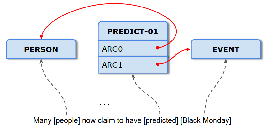
Key to our setup is the interpretation of each neuron in a DNN as an activation vector. As shown in the figure below, the activation vector of a neuron is the scalar output it produces on the input data. For example, for 50 input images, a neuron in a DNN will output 50 scalar values, encoding how much it responds to each input. These 50 scalar values then make up an activation vector for the neuron. (Of course, in practice, we take many more than 50 inputs.)
Here a DNN is given three inputs, x1, x2, x3. Looking at a neuron inside the DNN (bolded in red, right pane), this neuron produces a scalar output zi corresponding to each input xi. These values form the activation vector of the neuron.
With this basic observation and a little more formulation, we introduce Singular Vector Canonical Correlation Analysis (SVCCA), a technique for taking in two sets of neurons and outputting aligned feature maps learned by both of them. Critically, this technique accounts for superficial differences such as permutations in neuron orderings (crucial for comparing different networks), and can detect similarities where other, more straightforward comparisons fail.

As an example, consider training two convolutional neural nets (net1 and net2, below) on 
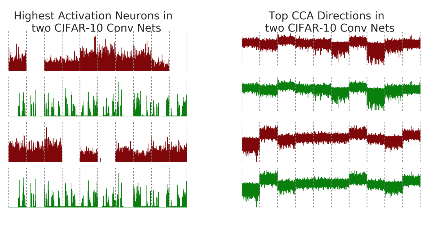
CIFAR-10, a medium scale image classification task. To visualize the results of our method, we compare activation vectors of neurons with the aligned features output by SVCCA. Recall that the activation vector of a neuron is the raw scalar outputs on input images. The x-axis of the plot consists of images sorted by class (gray dotted lines showing class boundaries), and the y axis the output value of the neuron.
On the left pane, we show the two highest activation (largest euclidean norm) neurons in net1 and net2. Examining highest activations neurons has been a popular method to interpret DNNs in computer vision, but in this case, the highest activation neurons in net1 and net2 have no clear correspondence, despite both being trained on the same task. However, after applying SVCCA, (right pane), we see that the latent representations learned by both networks do indeed share some very similar features. Note that the top two rows representing aligned feature maps are close to identical, as are the second highest aligned feature maps (bottom two rows). Furthermore, these aligned mappings in the right pane also show a clear correspondence with the class boundaries, e.g. we see the top pair give negative outputs for Class 8, with the bottom pair giving a positive output for Class 2 and Class 7.

While you can apply SVCCA across networks, one can also do this for the same network, across time, enabling the study of how different layers in a network converge to their final representations. Below, we show panes that compare the representation of layers in net1 during training (y-axes) with the layers at the end of training (x-axes). For example, in the top left pane (titled “0% trained”), the x-axis shows layers of increasing depth of net1 at 100% trained, and the y axis shows layers of increasing depth at 0% trained. Each (i,j) square then tells us how similar the representation of layer i at 100% trained is to layer j at 0% trained. The input layer is at the bottom left, and is (as expected) identical at 0% to 100%. We make this comparison at several points through training, at 0%, 35%, 75% and 100%, for convolutional (top row) and residual (bottom row) nets on CIFAR-10.
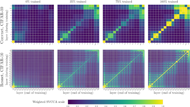
Plots showing learning dynamics of convolutional and residual networks on CIFAR-10. Note the additional structure also visible: the 2x2 blocks in the top row are due to batch norm layers, and the checkered pattern in the bottom row due to residual connections.
We find evidence of bottom-up convergence, with layers closer to the input converging first, and layers higher up taking longer to converge. This suggests a faster training method, Freeze Training — see our paper for details. Furthermore, this visualization also helps highlight properties of the network. In the top row, there are a couple of 2x2 blocks. These correspond to batch normalization layers, which are representationally identical to their previous layers. On the bottom row, towards the end of training, we can see a checkerboard like pattern appear, which is due to the residual connections of the network having greater similarity to previous layers.

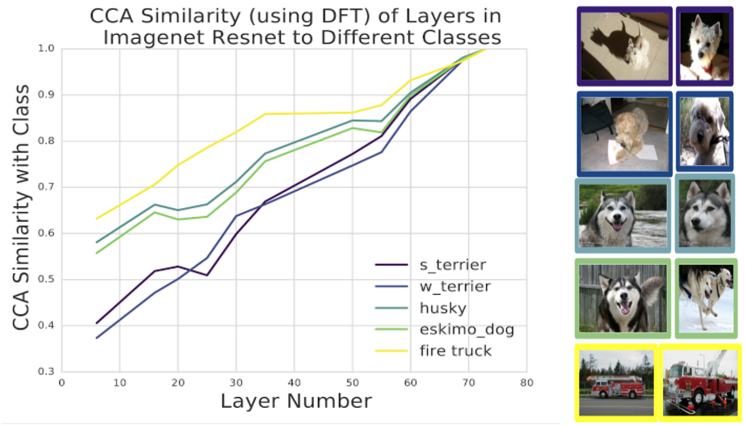
So far, we’ve concentrated on applying SVCCA to CIFAR-10. But applying preprocessing techniques with the Discrete Fourier transform, we can scale this method to Imagenet sized models. We applied this technique to the Imagenet Resnet, comparing the similarity of latent representations to representations corresponding to different classes:
SVCCA similarity of latent representations with different classes. We take different layers in Imagenet Resnet, with 0 indicating input and 74 indicating output, and compare representational similarity of the hidden layer and the output class. Interestingly, different classes are learned at different speeds: the firetruck class is learned faster than the different dog breeds. Furthermore, the two pairs of dog breeds (a husky-like pair and a terrier-like pair) are learned at the same rate, reflecting the visual similarity between them.
Our paper gives further details on the results we’ve explored so far, and also touches on different applications, e.g. compressing DNNs by projecting onto the SVCCA outputs, and Freeze Training, a computationally cheaper method for training deep networks. There are many followups we’re excited about exploring with SVCCA — moving on to different kinds of architectures, comparing across datasets, and better visualizing the aligned directions are just a few ideas we’re eager to try out. We look forward to presenting these results next week at NIPS 2017 in Long Beach, and we hope the code will also encourage many people to apply SVCCA to their network representations to interpret and understand what their network is learning.

Understanding Medical Conversations


Good documentation helps create good clinical care by communicating a doctor's thinking, their concerns, and their plans to the rest of the team. Unfortunately, physicians routinely spend more time doing documentation than doing what they love most — caring for patients. Part of the reason is that doctors spend ~6 hours in an 11-hour workday in the Electronic Health Records (EHR) on documentation.1 Consequently, one study found that more than half of surveyed doctors report at least one symptom of burnout.2

In order to help offload note-taking, many doctors have started using medical scribes as a part of their workflow. These scribes listen to the patient-doctor conversations and create notes for the EHR. According to a recent study, introducing scribes not only improved physician satisfaction, but also medical chart quality and accuracy.3 But the number of doctor-patient conversations that need a scribe is far beyond the capacity of people who are available for medical scribing.

We wondered: could the voice recognition technologies already available in Google Assistant, Google Home, and Google Translate be used to document patient-doctor conversations and help doctors and scribes summarize notes more quickly?
In “Speech Recognition for Medical Conversations”, we show that it is possible to build Automatic Speech Recognition (ASR) models for transcribing medical conversations. While most of the current ASR solutions in medical domain focus on transcribing doctor dictations (i.e., single speaker speech consisting of predictable medical terminology), our research shows that it is possible to build an ASR model which can handle multiple speaker conversations covering everything from weather to complex medical diagnosis.

Using this technology, we will start working with physicians and researchers at Stanford University, who have done extensive research on how scribes can improve physician satisfaction, to understand how deep learning techniques such as ASR can facilitate the scribing process of physician notes. In our pilot study, we investigate what types of clinically relevant information can be extracted from medical conversations to assist physicians in reducing their interactions with the EHR. The study is fully patient-consented and the content of the recording will be de-identified to protect patient privacy.

We hope these technologies will not only help return joy to practice by facilitating doctors and scribes with their everyday workload, but also help the patients get more dedicated and thorough medical attention, ideally, leading to better care.


1 http://www.annfammed.org/content/15/5/419.full
2 http://www.mayoclinicproceedings.org/article/S0025-6196%2815%2900716-8/abstract
3 http://www.annfammed.org/content/15/5/427.full

SLING: A Natural Language Frame Semantic Parser


Until recently, most practical natural language understanding (NLU) systems used a pipeline of analysis stages, from part-of-speech tagging and dependency parsing to steps that computed a semantic representation of the input text. While this facilitated easy modularization of different analysis stages, errors in earlier stages would have cascading effects in later stages and the final representation, and the intermediate stage outputs might not be relevant on their own. For example, a typical pipeline might perform the task of dependency parsing in an early stage and the task of coreference resolution towards the end. If one was only interested in the output of coreference resolution, it would be affected by cascading effects of any errors during dependency parsing.

Today we are announcing SLING, an experimental system for parsing natural language text directly into a representation of its meaning as a semantic frame graph. The output frame graph directly captures the semantic annotations of interest to the user, while avoiding the pitfalls of pipelined systems by not running any intermediate stages, additionally preventing unnecessary computation. SLING uses a special-purpose recurrent neural network model to compute the output representation of input text through incremental editing operations on the frame graph. The frame graph, in turn, is flexible enough to capture many semantic tasks of interest (more on this below). SLING's parser is trained using only the input words, bypassing the need for producing any intermediate annotations (e.g. dependency parses).

SLING provides fast parsing at inference time by providing (a) an efficient and scalable frame store implementation and (b) a JIT compiler that generates efficient code to execute the recurrent neural network. Although SLING is experimental, it achieves a parsing speed of >2,500 tokens/second on a desktop CPU, thanks to its efficient frame store and neural network compiler. SLING is implemented in C++ and it is available for download on GitHub. The entire system is described in detail in a technical report as well.

Frame Semantic Parsing
Frame Semantics [1] represents the meaning of text — such as a sentence — as a set of formal statements. Each formal statement is called a frame, which can be seen as a unit of knowledge or meaning, that also contains interactions with concepts or other frames typically associated with it. SLING organizes each frame as a list of slots, where each slot has a name (role) and a value which could be a literal or a link to another frame. As an example, consider the sentence:

“Many people now claim to have predicted Black Monday.”

The figure below illustrates SLING recognizing mentions of entities (e.g. people, places, or events), measurements (e.g. dates or distances), and other concepts (e.g. verbs), and placing them in the correct semantic roles for the verbs in the input. The word predicted evokes the most dominant sense of the verb "predict", denoted as a PREDICT-01 frame. Additionally, this frame also has interactions (slots) with who made the prediction (denoted via the ARG0 slot, which points to the PERSON frame for people) and what was being predicted (denoted via ARG1, which links to the EVENT frame for Black Monday). Frame semantic parsing is the task of producing a directed graph of such frames linked through slots.
Although the example above is fairly simple, frame graphs are powerful enough to model a variety of complex semantic annotation tasks. For starters, frames provide a convenient way to bring together language-internal and external information types (e.g. knowledge bases). This can then be used to address complex language understanding problems such as reference, metaphor, metonymy, and perspective. The frame graphs for these tasks only differ in the inventory of frame types, roles, and any linking constraints.

SLING
SLING trains a recurrent neural network by optimizing for the semantic frames of interest.
The internal learned representations in the network’s hidden layers replace the hand-crafted feature combinations and intermediate representations in pipelined systems. Internally, SLING uses an encoder-decoder architecture where each input word is encoded into a vector using simple lexical features like the raw word, its suffix(es), punctuation etc. The decoder uses that representation, along with recurrent features from its own history, to compute a sequence of transitions that update the frame graph to obtain the intended frame semantic representation of the input sentence. SLING trains its model using TensorFlow and DRAGNN.

The animation below shows how frames and roles are incrementally added to the under-construction frame graph using individual transitions. As discussed earlier with our simple example sentence, SLING connects the VERB and EVENT frames using the role ARG1, signifying that the EVENT frame is the concept being predicted. The EVOKE transition evokes a frame of a specified type from the next few tokens in the text (e.g. EVENT from Black Monday). Similarly, the CONNECT transition links two existing frames with a specified role. When the input is exhausted and the last transition (denoted as STOP) is executed, the frame graph is deemed as complete and returned to the user, who can inspect the graph to get the semantic meaning behind the sentence.
One key aspect of our transition system is the presence of a small fixed-size attention buffer of frames that represents the most recent frames to be evoked or modified, shown with the orange boxes in the figure above. This buffer captures the intuition that we tend to remember knowledge that was recently evoked, referred to, or enhanced. If a frame is no longer in use, it eventually gets flushed out of this buffer as new frames come into picture. We found this simple mechanism to be surprisingly effective at capturing a large fraction of inter-frame links.

Next Steps
The illustrative experiment above is just a launchpad for research in semantic parsing for tasks such as knowledge extraction, resolving complex references, and dialog understanding. The SLING release on Github comes with a pre-trained model for the task we illustrated, as well as examples and recipes to train your own parser on either the supplied synthetic data or your own data. We hope the community finds SLING useful and we look forward to engaging conversations about applying and extending SLING to other semantic parsing tasks.

Acknowledgements
The research described in this post was done by Michael Ringgaard, Rahul Gupta, and Fernando Pereira. We thank the Tensorflow and DRAGNN teams for open-sourcing their packages, and various colleagues at DRAGNN who helped us with multiple aspects of SLING's training setup.


1 Charles J. Fillmore. 1982. Frame semantics. Linguistics in the Morning Calm, pages 111–138.

On-Device Conversational Modeling with TensorFlow Lite


Earlier this year, we launched Android Wear 2.0 which featured the first "on-device" machine learning technology for smart messaging. This enabled cloud-based technologies like Smart Reply, previously available in Gmail, Inbox and Allo, to be used directly within any application for the first time, including third-party messaging apps, without ever having to connect to the cloud. So you can respond to incoming chat messages on the go, directly from your smartwatch.

Today, we announce TensorFlow Lite, TensorFlow’s lightweight solution for mobile and embedded devices. This framework is optimized for low-latency inference of machine learning models, with a focus on small memory footprint and fast performance. As part of the library, we have also released an on-device conversational model and a demo app that provides an example of a natural language application powered by TensorFlow Lite, in order to make it easier for developers and researchers to build new machine intelligence features powered by on-device inference. This model generates reply suggestions to input conversational chat messages, with efficient inference that can be easily plugged in to your chat application to power on-device conversational intelligence.

The on-device conversational model we have released uses a new ML architecture for training compact neural networks (as well as other machine learning models) based on a joint optimization framework, originally presented in ProjectionNet: Learning Efficient On-Device Deep Networks Using Neural Projections. This architecture can run efficiently on mobile devices with limited computing power and memory, by using efficient “projection” operations that transform any input to a compact bit vector representation — similar inputs are projected to nearby vectors that are dense or sparse depending on type of projection. For example, the messages “hey, how's it going?” and “How's it going buddy?”, might be projected to the same vector representation.

Using this idea, the conversational model combines these efficient operations at low computation and memory footprint. We trained this on-device model end-to-end using an ML framework that jointly trains two types of models — a compact projection model (as described above) combined with a trainer model. The two models are trained in a joint fashion, where the projection model learns from the trainer model — the trainer is characteristic of an expert and modeled using larger and more complex ML architectures, whereas the projection model resembles a student that learns from the expert. During training, we can also stack other techniques such as quantization or distillation to achieve further compression or selectively optimize certain portions of the objective function. Once trained, the smaller projection model is able to be used directly for inference on device.
For inference, the trained projection model is compiled into a set of TensorFlow Lite operations that have been optimized for fast execution on mobile platforms and executed directly on device. The TensorFlow Lite inference graph for the on-device conversational model is shown here.
TensorFlow Lite execution for the On-Device Conversational Model.
The open-source conversational model released today (along with code) was trained end-to-end using the joint ML architecture described above. Today’s release also includes a demo app, so you can easily download and try out one-touch smart replies on your mobile device. The architecture enables easy configuration for model size and prediction quality based on application needs. You can find a list of sample messages where this model does well here. The system can also fall back to suggesting replies from a fixed set that was learned and compiled from popular response intents observed in chat conversations. The underlying model is different from the ones Google uses for Smart Reply responses in its apps1.

Beyond Conversational Models
Interestingly, the ML architecture described above permits flexible choices for the underlying model. We also designed the architecture to be compatible with different machine learning approaches — for example, when used with TensorFlow deep learning, we learn a lightweight neural network (ProjectionNet) for the underlying model, whereas a different architecture (ProjectionGraph) represents the model using a graph framework instead of a neural network.

The joint framework can also be used to train lightweight on-device models for other tasks using different ML modeling architectures. As an example, we derived a ProjectionNet architecture that uses a complex feed-forward or recurrent architecture (like LSTM) for the trainer model coupled with a simple projection architecture comprised of dynamic projection operations and a few, narrow fully-connected layers. The whole architecture is trained end-to-end using backpropagation in TensorFlow and once trained, the compact ProjectionNet is directly used for inference. Using this method, we have successfully trained tiny ProjectionNet models that achieve significant reduction in model sizes (up to several orders of magnitude reduction) and high performance with respect to accuracy on multiple visual and language classification tasks (a few examples here). Similarly, we trained other lightweight models using our graph learning framework, even in semi-supervised settings.
ML architecture for training on-device models: ProjectionNet trained using deep learning (left), and ProjectionGraph trained using graph learning (right).
We will continue to improve and release updated TensorFlow Lite models in open-source. We think that the released model (as well as future models) learned using these ML architectures may be reused for many natural language and computer vision applications or plugged into existing apps for enabling machine intelligence. We hope that the machine learning and natural language processing communities will be able to build on these to address new problems and use-cases we have not yet conceived.

Acknowledgments
Yicheng Fan and Gaurav Nemade contributed immensely to this effort. Special thanks to Rajat Monga, Andre Hentz, Andrew Selle, Sarah Sirajuddin, and Anitha Vijayakumar from the TensorFlow team; Robin Dua, Patrick McGregor, Andrei Broder, Andrew Tomkins and the Google Expander team.


1 The released on-device model was trained to optimize for small size and low latency applications on mobile phones and wearables. Smart Reply predictions in Google apps, however are generated using larger, more complex models. In production systems, we also use multiple classifiers that are trained to detect inappropriate content and apply further filtering and tuning to optimize user experience and quality levels. We recommend that developers using the open-source TensorFlow Lite version also follow such practices for their end applications.