Author Archives: Research Blog

Introducing the iNaturalist 2018 Challenge


Thanks to recent advances in deep learning, the visual recognition abilities of machines have improved dramatically, permitting the practical application of computer vision to tasks ranging from pedestrian detection for self-driving cars to expression recognition in virtual reality. One area that remains challenging for computers, however, is fine-grained and instance-level recognition. Earlier this month, we posted an instance-level landmark recognition challenge for identifying individual landmarks. Here we focus on fine-grained visual recognition, which is to distinguish species of animals and plants, car and motorcycle models, architectural styles, etc. For computers, discriminating fine-grained categories is challenging because many categories have relatively few training examples (i.e., the long tail problem), the examples that do exist often lack authoritative training labels, and there is variability in illumination, viewing angle and object occlusion.

To help confront these hurdles, we are excited to announce the 2018 iNaturalist Challenge (iNat-2018), a species classification competition offered in partnership with iNaturalist and Visipedia (short for Visual Encyclopedia), a project for which Caltech and Cornell Tech received a Google Focused Research Award. This is a flagship challenge for the 5th International Workshop on Fine Grained Visual Categorization (FGVC5) at CVPR 2018. Building upon the first iNaturalist challenge, iNat-2017, iNat-2018 spans over 8000 categories of plants, animals, and fungi, with a total of more than 450,000 training images. We invite participants to enter the competition on Kaggle, with final submissions due in early June. Training data, annotations, and links to pretrained models can be found on our GitHub repo.

iNaturalist has emerged as a world leader for citizen scientists to share observations of species and connect with nature since its founding in 2008. It hosts research-grade photos and annotations submitted by a thriving, engaged community of users. Consider the following photo from iNaturalist:
The map on the right shows where the photo was taken. Image credit: Serge Belongie.
You may notice that the photo on the left contains a turtle. But did you also know this is a Trachemys scripta, common name “Pond Slider?” If you knew the latter, you possess knowledge of fine-grained or subordinate categories.

In contrast to other image classification datasets such as ImageNet, the dataset in the iNaturalist challenge exhibits a long-tailed distribution, with many species having relatively few images. It is important to enable machine learning models to handle categories in the long-tail, as the natural world is heavily imbalanced – some species are more abundant and easier to photograph than others. The iNaturalist challenge will encourage progress because the training distribution of iNat-2018 has an even longer tail than iNat-2017.
Distribution of training images per species for iNat-2017 and iNat-2018, plotted on a log-log scale, illustrating the long-tail behavior typical of fine-grained classification problems. Image Credit: Grant Van Horn and Oisin Mac Aodha.
Along with iNat-2018, FGVC5 will also host the iMaterialist 2018 challenge (including a furniture categorization challenge and a fashion attributes challenge for product images) and a set of “FGVCx” challenges representing smaller scale – but still significant – challenges, featuring content such as food and modern art.

FGVC5 will be showcased on the main stage at CVPR 2018, thereby ensuring broad exposure for the top performing teams. This project will advance the state-of-the-art in automatic image classification for real world, fine-grained categories, with heavy class imbalances, and large numbers of classes. We cordially invite you to participate in these competitions and help move the field forward!

Acknowledgements
We’d like to thank our colleagues and friends at iNaturalist, Visipedia, and FGVC5 for working together to advance this important area. At Google we would like to thank Hartwig Adam, Weijun Wang, Nathan Frey, Andrew Howard, Alessandro Fin, Yuning Chai, Xiao Zhang, Jack Sim, Yuan Li, Grant Van Horn, Yin Cui, Chen Sun, Yanan Qian, Grace Vesom, Tanya Birch, Wendy Kan, and Maggie Demkin.

Open Sourcing the Hunt for Exoplanets


Recently, we discovered two exoplanets by training a neural network to analyze data from NASA’s Kepler space telescope and accurately identify the most promising planet signals. And while this was only an initial analysis of ~700 stars, we consider this a successful proof-of-concept for using machine learning to discover exoplanets, and more generally another example of using machine learning to make meaningful gains in a variety of scientific disciplines (e.g. healthcare, quantum chemistry, and fusion research).

Today, we’re excited to release our code for processing the Kepler data, training our neural network model, and making predictions about new candidate signals. We hope this release will prove a useful starting point for developing similar models for other NASA missions, like K2 (Kepler’s second mission) and the upcoming Transiting Exoplanet Survey Satellite mission. As well as announcing the release of our code, we’d also like take this opportunity to dig a bit deeper into how our model works.

A Planet Hunting Primer
First, let’s consider how data collected by the Kepler telescope is used to detect the presence of a planet. The plot below is called a light curve, and it shows the brightness of the star (as measured by Kepler’s photometer) over time. When a planet passes in front of the star, it temporarily blocks some of the light, which causes the measured brightness to decrease and then increase again shortly thereafter, causing a “U-shaped” dip in the light curve.
A light curve from the Kepler space telescope with a “U-shaped” dip that indicates a transiting exoplanet.
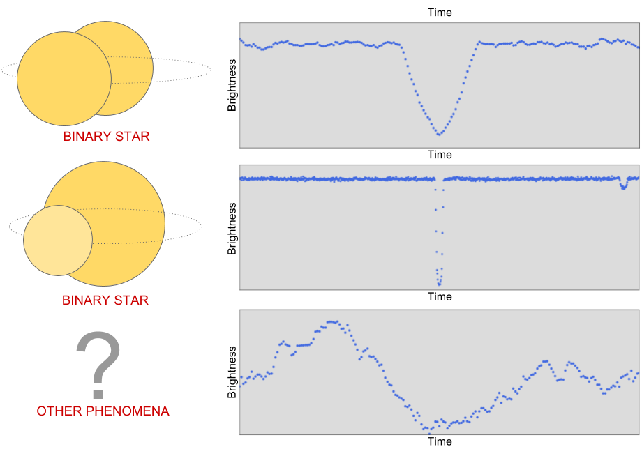
However, other astronomical and instrumental phenomena can also cause the measured brightness of a star to decrease, including binary star systems, starspots, cosmic ray hits on Kepler’s photometer, and instrumental noise.
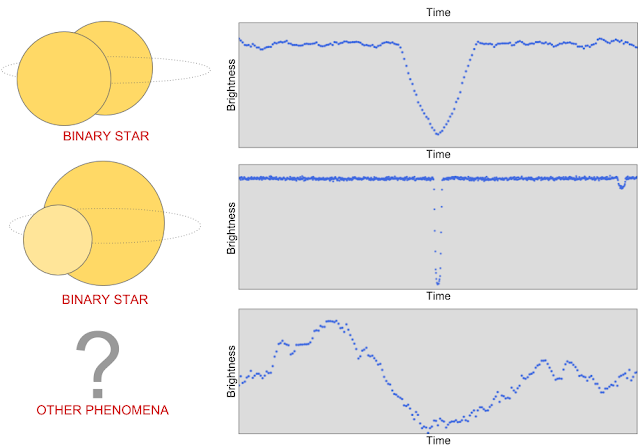
The first light curve has a “V-shaped” pattern that tells us that a very large object (i.e. another star) passed in front of the star that Kepler was observing. The second light curve contains two places where the brightness decreases, which indicates a binary system with one bright and one dim star: the larger dip is caused by the dimmer star passing in front of the brighter star, and vice versa. The third light curve is one example of the many other non-planet signals where the measured brightness of a star appears to decrease.
To search for planets in Kepler data, scientists use automated software (e.g. the Kepler data processing pipeline) to detect signals that might be caused by planets, and then manually follow up to decide whether each signal is a planet or a false positive. To avoid being overwhelmed with more signals than they can manage, the scientists apply a cutoff to the automated detections: those with signal-to-noise ratios above a fixed threshold are deemed worthy of follow-up analysis, while all detections below the threshold are discarded. Even with this cutoff, the number of detections is still formidable: to date, over 30,000 detected Kepler signals have been manually examined, and about 2,500 of those have been validated as actual planets!

Perhaps you’re wondering: does the signal-to-noise cutoff cause some real planet signals to be missed? The answer is, yes! However, if astronomers need to manually follow up on every detection, it’s not really worthwhile to lower the threshold, because as the threshold decreases the rate of false positive detections increases rapidly and actual planet detections become increasingly rare. However, there’s a tantalizing incentive: it’s possible that some potentially habitable planets like Earth, which are relatively small and orbit around relatively dim stars, might be hiding just below the traditional detection threshold — there might be hidden gems still undiscovered in the Kepler data!

A Machine Learning Approach
The Google Brain team applies machine learning to a diverse variety of data, from human genomes to sketches to formal mathematical logic. Considering the massive amount of data collected by the Kepler telescope, we wondered what we might find if we used machine learning to analyze some of the previously unexplored Kepler data. To find out, we teamed up with Andrew Vanderburg at UT Austin and developed a neural network to help search the low signal-to-noise detections for planets.
We trained a convolutional neural network (CNN) to predict the probability that a given Kepler signal is caused by a planet. We chose a CNN because they have been very successful in other problems with spatial and/or temporal structure, like audio generation and image classification.
Luckily, we had 30,000 Kepler signals that had already been manually examined and classified by humans. We used a subset of around 15,000 of these signals, of which around 3,500 were verified planets or strong planet candidates, to train our neural network to distinguish planets from false positives. The inputs to our network are two separate views of the same light curve: a wide view that allows the model to examine signals elsewhere on the light curve (e.g., a secondary signal caused by a binary star), and a zoomed-in view that enables the model to closely examine the shape of the detected signal (e.g., to distinguish “U-shaped” signals from “V-shaped” signals).

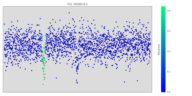
Once we had trained our model, we investigated the features it learned about light curves to see if they matched with our expectations. One technique we used (originally suggested in this paper) was to systematically occlude small regions of the input light curves to see whether the model’s output changed. Regions that are particularly important to the model’s decision will change the output prediction if they are occluded, but occluding unimportant regions will not have a significant effect. Below is a light curve from a binary star that our model correctly predicts is not a planet. The points highlighted in green are the points that most change the model’s output prediction when occluded, and they correspond exactly to the secondary “dip” indicative of a binary system. When those points are occluded, the model’s output prediction changes from ~0% probability of being a planet to ~40% probability of being a planet. So, those points are part of the reason the model rejects this light curve, but the model uses other evidence as well - for example, zooming in on the centred primary dip shows that it's actually “V-shaped”, which is also indicative of a binary system.
Searching for New Planets
Once we were confident with our model’s predictions, we tested its effectiveness by searching for new planets in a small set 670 stars. We chose these stars because they were already known to have multiple orbiting planets, and we believed that some of these stars might host additional planets that had not yet been detected. Importantly, we allowed our search to include signals that were below the signal-to-noise threshold that astronomers had previously considered. As expected, our neural network rejected most of these signals as spurious detections, but a handful of promising candidates rose to the top, including our two newly discovered planets: Kepler-90 i and Kepler-80 g.

Find your own Planet(s)!
Let’s take a look at how the code released today can help (re-)discover the planet Kepler-90 i. The first step is to train a model by following the instructions on the code’s home page. It takes a while to download and process the data from the Kepler telescope, but once that’s done, it’s relatively fast to train a model and make predictions about new signals. One way to find new signals to show the model is to use an algorithm called Box Least Squares (BLS), which searches for periodic “box shaped” dips in brightness (see below). The BLS algorithm will detect “U-shaped” planet signals, “V-shaped” binary star signals and many other types of false positive signals to show the model. There are various freely available software implementations of the BLS algorithm, including VARTOOLS and LcTools. Alternatively, you can even look for candidate planet transits by eye, like the Planet Hunters.
A low signal-to-noise detection in the light curve of the Kepler 90 star detected by the BLS algorithm. The detection has period 14.44912 days, duration 2.70408 hours (0.11267 days) beginning 2.2 days after 12:00 on 1/1/2009 (the year the Kepler telescope launched).
To run this detected signal though our trained model, we simply execute the following command:
python predict.py  --kepler_id=11442793 --period=14.44912 --t0=2.2
--duration=0.11267 --kepler_data_dir=$HOME/astronet/kepler
--output_image_file=$HOME/astronet/kepler-90i.png
--model_dir=$HOME/astronet/model
The output of the command is prediction = 0.94, which means the model is 94% certain that this signal is a real planet. Of course, this is only a small step in the overall process of discovering and validating an exoplanet: the model’s prediction is not proof one way or the other. The process of validating this signal as a real exoplanet requires significant follow-up work by an expert astronomer — see Sections 6.3 and 6.4 of our paper for the full details. In this particular case, our follow-up analysis validated this signal as a bona fide exoplanet, and it’s now called Kepler-90 i!
Our work here is far from done. We’ve only searched 670 stars out of 200,000 observed by Kepler — who knows what we might find when we turn our technique to the entire dataset. Before we do that, though, we have a few improvements we want to make to our model. As we discussed in our paper, our model is not yet as good at rejecting binary stars and instrumental false positives as some more mature computer heuristics. We’re hard at work improving our model, and now that it’s open sourced, we hope others will do the same!

If you’d like to learn more, Chris is featured on the latest episode of This Week In Machine Learning & AI discussing his work.

The Building Blocks of Interpretability


(Crossposted on the Google Open Source Blog)

In 2015, our early attempts to visualize how neural networks understand images led to psychedelic images. Soon after, we open sourced our code as DeepDream and it grew into a small art movement producing all sorts of amazing things. But we also continued the original line of research behind DeepDream, trying to address one of the most exciting questions in Deep Learning: how do neural networks do what they do?

Last year in the online journal Distill, we demonstrated how those same techniques could show what individual neurons in a network do, rather than just what is “interesting to the network” as in DeepDream. This allowed us to see how neurons in the middle of the network are detectors for all sorts of things — buttons, patches of cloth, buildings — and see how those build up to be more and more sophisticated over the networks layers.
Visualizations of neurons in GoogLeNet. Neurons in higher layers represent higher level ideas.
While visualizing neurons is exciting, our work last year was missing something important: how do these neurons actually connect to what the network does in practice?

Today, we’re excited to publish “The Building Blocks of Interpretability,” a new Distill article exploring how feature visualization can combine together with other interpretability techniques to understand aspects of how networks make decisions. We show that these combinations can allow us to sort of “stand in the middle of a neural network” and see some of the decisions being made at that point, and how they influence the final output. For example, we can see things like how a network detects a floppy ear, and then that increases the probability it gives to the image being a “Labrador retriever” or “beagle”.

We explore techniques for understanding which neurons fire in the network. Normally, if we ask which neurons fire, we get something meaningless like “neuron 538 fired a little bit,” which isn’t very helpful even to experts. Our techniques make things more meaningful to humans by attaching visualizations to each neuron, so we can see things like “the floppy ear detector fired”. It’s almost a kind of MRI for neural networks.
We can also zoom out and show how the entire image was “perceived” at different layers. This allows us to really see the transition from the network detecting very simple combinations of edges, to rich textures and 3d structure, to high-level structures like ears, snouts, heads and legs.
These insights are exciting by themselves, but they become even more exciting when we can relate them to the final decision the network makes. So not only can we see that the network detected a floppy ear, but we can also see how that increases the probability of the image being a labrador retriever.
In addition to our paper, we’re also releasing Lucid, a neural network visualization library building off our work on DeepDream. It allows you to make the sort lucid feature visualizations we see above, in addition to more artistic DeepDream images.

We’re also releasing colab notebooks. These notebooks make it extremely easy to use Lucid to reproduce visualizations in our article! Just open the notebook, click a button to run code — no setup required!
In colab notebooks you can click a button to run code, and see the result below.
This work only scratches the surface of the kind of interfaces that we think it’s possible to build for understanding neural networks. We’re excited to see what the community will do — and we’re excited to work together towards deeper human understanding of neural networks.

A Preview of Bristlecone, Google’s New Quantum Processor


The goal of the Google Quantum AI lab is to build a quantum computer that can be used to solve real-world problems. Our strategy is to explore near-term applications using systems that are forward compatible to a large-scale universal error-corrected quantum computer. In order for a quantum processor to be able to run algorithms beyond the scope of classical simulations, it requires not only a large number of qubits. Crucially, the processor must also have low error rates on readout and logical operations, such as single and two-qubit gates.

Today we presented Bristlecone, our new quantum processor, at the annual American Physical Society meeting in Los Angeles. The purpose of this gate-based superconducting system is to provide a testbed for research into system error rates and scalability of our qubit technology, as well as applications in quantum simulation, optimization, and machine learning.
Bristlecone is Google’s newest quantum processor (left). On the right is a cartoon of the device: each “X” represents a qubit, with nearest neighbor connectivity.
The guiding design principle for this device is to preserve the underlying physics of our previous 9-qubit linear array technology1, 2, which demonstrated low error rates for readout (1%), single-qubit gates (0.1%) and most importantly two-qubit gates (0.6%) as our best result. This device uses the same scheme for coupling, control, and readout, but is scaled to a square array of 72 qubits. We chose a device of this size to be able to demonstrate quantum supremacy in the future, investigate first and second order error-correction using the surface code, and to facilitate quantum algorithm development on actual hardware.
2D conceptual chart showing the relationship between error rate and number of qubits. The intended research direction of the Quantum AI Lab is shown in red, where we hope to access near-term applications on the road to building an error corrected quantum computer.
Before investigating specific applications, it is important to quantify a quantum processor’s capabilities. Our theory team has developed a benchmarking tool for exactly this task. We can assign a single system error by applying random quantum circuits to the device and checking the sampled output distribution against a classical simulation. If a quantum processor can be operated with low enough error, it would be able to outperform a classical supercomputer on a well-defined computer science problem, an achievement known as quantum supremacy. These random circuits must be large in both number of qubits as well as computational length (depth). Although no one has achieved this goal yet, we calculate quantum supremacy can be comfortably demonstrated with 49 qubits, a circuit depth exceeding 40, and a two-qubit error below 0.5%. We believe the experimental demonstration of a quantum processor outperforming a supercomputer would be a watershed moment for our field, and remains one of our key objectives.
A Bristlecone chip being installed by Research Scientist Marissa Giustina at the Quantum AI Lab in Santa Barbara
We are looking to achieve similar performance to the best error rates of the 9-qubit device, but now across across all 72 qubits of Bristlecone. We believe Bristlecone would then be a compelling proof-of-principle for building larger scale quantum computers. Operating a device such as Bristlecone at low system error requires harmony between a full stack of technology ranging from software and control electronics to the processor itself. Getting this right requires careful systems engineering over several iterations.

We are cautiously optimistic that quantum supremacy can be achieved with Bristlecone, and feel that learning to build and operate devices at this level of performance is an exciting challenge! We look forward to sharing the results and allowing collaborators to run experiments in the future.

Making Healthcare Data Work Better with Machine Learning


Over the past 10 years, healthcare data has moved from being largely on paper to being almost completely digitized in electronic health records. But making sense of this data involves a few key challenges. First, there is no common data representation across vendors; each uses a different way to structure their data. Second, even sites that use the same vendor may differ significantly, for example, they typically use different codes for the same medication. Third, data can be spread over many tables, some containing encounters, some containing lab results, and yet others containing vital signs.

The Fast Healthcare Interoperability Resources (FHIR) standard addresses most of these challenges: it has a solid yet extensible data-model, is built on established Web standards, and is rapidly becoming the de-facto standard for both individual records and bulk-data access. But to enable large-scale machine learning, we needed a few additions: implementations in various programming languages, an efficient way to serialize large amounts of data to disk, and a representation that allows analyses of large datasets.

Today, we are happy to open source a protocol buffer implementation of the FHIR standard, which addresses these issues. The current version supports Java, and support for C++, Go, and Python will follow soon. Support for profiles will follow shortly as well, plus tools to help convert legacy data into FHIR.

FHIR as the core data model
Over the past few years, as we’ve been partnering with academic medical centers to apply machine learning to de-identified medical records, it became clear that we needed to address the complexity of healthcare data head-on. Indeed, for machine learning to be effective on medical data, we need a holistic view of what happened to each patient over time. And as a bonus, we want a data representation that is directly applicable in a clinical setting.

While the FHIR standard addresses most of our needs, making healthcare data substantially easier to manage than “legacy” data structures and enabling large-scale machine-learning independent of vendors, we believe the introduction of protocol buffers can help both application developers and (machine-learning) researchers use FHIR.

Current release of protocol buffers
We’ve taken care to make our protocol buffer representation suitable for both programmatic access and database queries. One of the provided examples shows how to upload FHIR data into Google Cloud BigQuery and have it available for querying, and we are adding other examples that upload directly from bulk data export. Our protocol buffers adhere to the FHIR standard (they are in fact auto-generated from it) but make for more elegant queries.

The current release does not yet include support for training TensorFlow models, but keep an eye out for future updates. We aim to open-source as much as possible of our recent work, to help make our research more reproducible and applicable to real-world scenarios. Furthermore, we are working closely with our colleagues in Google Cloud on more tools for managing healthcare data at scale.

Acknowledgements
We enjoyed great discussions and helpful feedback from the FHIR community, including Grahame Grieve, Ewout Kramer, Josh Mandel and others. Thanks to our colleagues at DeepMind, the Google Brain team and our academic collaborators.

Mobile Real-time Video Segmentation


Video segmentation is a widely used technique that enables movie directors and video content creators to separate the foreground of a scene from the background, and treat them as two different visual layers. By modifying or replacing the background, creators can convey a particular mood, transport themselves to a fun location or enhance the impact of the message. However, this operation has traditionally been performed as a time-consuming manual process (e.g. an artist rotoscoping every frame) or requires a studio environment with a green screen for real-time background removal (a technique referred to as chroma keying). In order to enable users to create this effect live in the viewfinder, we designed a new technique that is suitable for mobile phones.

Today, we are excited to bring precise, real-time, on-device mobile video segmentation to the YouTube app by integrating this technology into stories. Currently in limited beta, stories is YouTube’s new lightweight video format, designed specifically for YouTube creators. Our new segmentation technology allows creators to replace and modify the background, effortlessly increasing videos’ production value without specialized equipment.
Neural network video segmentation in YouTube stories.
To achieve this, we leverage machine learning to solve a semantic segmentation task using convolutional neural networks. In particular, we designed a network architecture and training procedure suitable for mobile phones focusing on the following requirements and constraints:
  • A mobile solution should be lightweight and run at least 10-30 times faster than existing state-of-the-art photo segmentation models. For real time inference, such a model needs to provide results at 30 frames per second.
  • A video model should leverage temporal redundancy (neighboring frames look similar) and exhibit temporal consistency (neighboring results should be similar)
  • High quality segmentation results require high quality annotations.
The Dataset
To provide high quality data for our machine learning pipeline, we annotated ten of thousands of images that captured a wide spectrum of foreground poses and background settings. Annotations consisted of pixel accurate locations of foreground elements such as hair, glass, neck, skin, lips, etc. and a general background label achieving a cross-validation result of 98% Intersection-Over-Union (IOU) of human annotator quality.
An example image from our dataset carefully annotated with nine labels - foreground elements are overlaid over the image.
Network Input
Our specific segmentation task is to compute a binary mask separating foreground from background for every input frame (three channels, RGB) of the video. Achieving temporal consistency of the computed masks across frames is key. Current methods that utilize LSTMs or GRUs to realize this are too computationally expensive for real-time applications on mobile phones. Instead we first pass the computed mask from the previous frame as a prior by concatenating it as a fourth channel to the current RGB input frame to achieve temporal consistency, as shown below:
The original frame (left) is separated in its three color channels and concatenated with the previous mask (middle). This is used as input to our neural network to predict the mask for the current frame (right).
Training Procedure
In video segmentation we need to achieve frame-to-frame temporal continuity, while also accounting for temporal discontinuities such as people suddenly appearing in the field of view of the camera. To train our model to robustly handle those use cases, we transform the annotated ground truth of each photo in several ways and use it as a previous frame mask:
  • Empty previous mask - Trains the network to work correctly for the first frame and new objects in scene. This emulates the case of someone appearing in the camera's frame.
  • Affine transformed ground truth mask - Minor transformations train the network to propagate and adjust to the previous frame mask. Major transformations train the network to understand inadequate masks and discard them.
  • Transformed image - We implement thin plate spline smoothing of the original image to emulate fast camera movements and rotations.
Our real-time video segmentation in action.
Network Architecture
With that modified input/output, we build on a standard hourglass segmentation network architecture by adding the following improvements:
  • We use big convolution kernels with large strides of four and above to detect object features on the high-resolution RGB input frame. Convolutions for layers with a small number of channels (as it is the case for the RGB input) are comparably cheap, so using big kernels here has almost no effect on the computational costs.
  • For speed gains, we aggressively downsample using large strides combined with skip connections like U-Net to restore low-level features during upsampling. For our segmentation model this technique results in a significant improvement of 5% IOU compared to using no skip connections.
    Hourglass segmentation network w/ skip connections.
  • For even further speed gains, we optimized default ResNet bottlenecks. In the literature authors tend to squeeze channels in the middle of the network by a factor of four (e.g. reducing 256 channels to 64 by using 64 different convolution kernels). However, we noticed that one can squeeze much more aggressively by a factor of 16 or 32 without significant quality degradation.
    ResNet bottleneck with large squeeze factor.
  • To refine and improve the accuracy of edges, we add several DenseNet layers on top of our network in full resolution similar to neural matting. This technique improves overall model quality by a slight 0.5% IOU, however perceptual quality of segmentation improves significantly.
The end result of these modifications is that our network runs remarkably fast on mobile devices, achieving 100+ FPS on iPhone 7 and 40+ FPS on Pixel 2 with high accuracy (realizing 94.8% IOU on our validation dataset), delivering a variety of smooth running and responsive effects in YouTube stories.
Our immediate goal is to use the limited rollout in YouTube stories to test our technology on this first set of effects. As we improve and expand our segmentation technology to more labels, we plan to integrate it into Google's broader Augmented Reality services.

Acknowledgements
A thank you to our team members who worked on the tech and this launch with us: Andrey Vakunov, Yury Kartynnik, Artsiom Ablavatski, Ivan Grishchenko, Matsvei Zhdanovich, Andrei Kulik, Camillo Lugaresi, John Kim, Ryan Bolyard, Wendy Huang, Michael Chang, Aaron La Lau, Willi Geiger, Tomer Margolin, John Nack and Matthias Grundmann.


Google-Landmarks: A New Dataset and Challenge for Landmark Recognition


Image classification technology has shown remarkable improvement over the past few years, exemplified in part by the Imagenet classification challenge, where error rates continue to drop substantially every year. In order to continue advancing the state of the art in computer vision, many researchers are now putting more focus on fine-grained and instance-level recognition problems – instead of recognizing general entities such as buildings, mountains and (of course) cats, many are designing machine learning algorithms capable of identifying the Eiffel Tower, Mount Fuji or Persian cats. However, a significant obstacle for research in this area has been the lack of large annotated datasets.

Today, we are excited to advance instance-level recognition by releasing Google-Landmarks, the largest worldwide dataset for recognition of human-made and natural landmarks. Google-Landmarks is being released as part of the Landmark Recognition and Landmark Retrieval Kaggle challenges, which will be the focus of the CVPR’18 Landmarks workshop. The dataset contains more than 2 million images depicting 30 thousand unique landmarks from across the world (their geographic distribution is presented below), a number of classes that is ~30x larger than what is available in commonly used datasets. Additionally, to spur research in this field, we are open-sourcing Deep Local Features (DELF), an attentive local feature descriptor that we believe is especially suited for this kind of task.

Geographic distribution of landmarks in our dataset.
Landmark recognition presents some noteworthy differences from other problems. For example, even within a large annotated dataset, there might not be much training data available for some of the less popular landmarks. Additionally, since landmarks are generally rigid objects which do not move, the intra-class variation is very small (in other words, a landmark’s appearance does not change that much across different images of it). As a result, variations only arise due to image capture conditions, such as occlusions, different viewpoints, weather and illumination, making this distinct from other image recognition datasets where images of a particular class (such as a dog) can vary much more. These characteristics are also shared with other instance-level recognition problems, such as artwork recognition — so we hope the new dataset can benefit research for other image recognition problems as well.

The two Kaggle challenges provide access to annotated data to help researchers address these problems. The recognition track challenge is to build models that recognize the correct landmark in a dataset of challenging test images, while the retrieval track challenges participants to retrieve images containing the same landmark.

A few examples of images from the Google-Landmarks dataset, including landmarks such as Big Ben, Sacre Coeur Basilica, the rock sculpture of Decebalus and the Megyeri Bridge, among others.
If you plan to be at CVPR this year, we hope you’ll attend the CVPR’18 Landmarks workshop. However, everyone is able to participate in the challenge, and access to the new dataset is available via the Kaggle website. We hope this resource is valuable to your research and we can’t wait to see the ideas you will come up with for recognizing landmarks!

Acknowledgments
Jack Sim, Will Cukierski, Maggie Demkin, Hartwig Adam, Bohyung Han, Shih-Fu Chang, Ondrej Chum, Torsten Sattler, Giorgos Tolias, Xu Zhang, Fernando Brucher, Marco Andreetto, Gursheesh Kour.

A Summary of the Google Zürich Algorithms & Optimization Workshop


Recently, we hosted a workshop on Algorithms and Optimization in our office in Zürich, with the goal of fostering collaboration between researchers from academia and Google by providing a forum to exchange ideas in machine learning theory and large-scale graph mining. As part of the topics discussed, we additionally highlighted our aim to build a group similar to the NYC algorithms research team in Google’s Zürich office.
Silvio Lattanzi presenting the work of the Graph Mining team
The workshop was structured in five sessions (see the full agenda here), each consisting of talks by attendees that touched the following research areas:
Overall, it was a great day with many excellent talks and with many opportunities for discussing interesting problems. All the presentations, including videos, can be found on our workshop website, here.

Assessing Cardiovascular Risk Factors with Computer Vision


Heart attacks, strokes and other cardiovascular (CV) diseases continue to be among the top public health issues. Assessing this risk is critical first step toward reducing the likelihood that a patient suffers a CV event in the future. To do this assessment, doctors take into account a variety of risk factors — some genetic (like age and sex), some with lifestyle components (like smoking and blood pressure). While most of these factors can be obtained by simply asking the patient, others factors, like cholesterol, require a blood draw. Doctors also take into account whether or not a patient has another disease, such as diabetes, which is associated with significantly increased risk of CV events.

Recently, we’ve seen many examples [1–4] of how deep learning techniques can help to increase the accuracy of diagnoses for medical imaging, especially for diabetic eye disease. In “Prediction of Cardiovascular Risk Factors from Retinal Fundus Photographs via Deep Learning,” published in Nature Biomedical Engineering, we show that in addition to detecting eye disease, images of the eye can very accurately predict other indicators of CV health. This discovery is particularly exciting because it suggests we might discover even more ways to diagnose health issues from retinal images.

Using deep learning algorithms trained on data from 284,335 patients, we were able to predict CV risk factors from retinal images with surprisingly high accuracy for patients from two independent datasets of 12,026 and 999 patients. For example, our algorithm could distinguish the retinal images of a smoker from that of a non-smoker 71% of the time. In addition, while doctors can typically distinguish between the retinal images of patients with severe high blood pressure and normal patients, our algorithm could go further to predict the systolic blood pressure within 11 mmHg on average for patients overall, including those with and without high blood pressure.
LEFT: image of the back of the eye showing the macula (dark spot in the middle), optic disc (bright spot at the right), and blood vessels (dark red lines arcing out from the bright spot on the right). RIGHT: retinal image in gray, with the pixels used by the deep learning algorithm to make predictions about the blood pressure highlighted in shades of green (heatmap). We found that each CV risk factor prediction uses a distinct pattern, such as blood vessels for blood pressure, and optic disc for other predictions.
In addition to predicting the various risk factors (age, gender, smoking, blood pressure, etc) from retinal images, our algorithm was fairly accurate at predicting the risk of a CV event directly. Our algorithm used the entire image to quantify the association between the image and the risk of heart attack or stroke. Given the retinal image of one patient who (up to 5 years) later experienced a major CV event (such as a heart attack) and the image of another patient who did not, our algorithm could pick out the patient who had the CV event 70% of the time. This performance approaches the accuracy of other CV risk calculators that require a blood draw to measure cholesterol.

More importantly, we opened the “black box” by using attention techniques to look at how the algorithm was making its prediction. These techniques allow us to generate a heatmap that shows which pixels were the most important for a predicting a specific CV risk factor. For example, the algorithm paid more attention to blood vessels for making predictions about blood pressure, as shown in the image above. Explaining how the algorithm is making its prediction gives doctor more confidence in the algorithm itself. In addition, this technique could help generate hypotheses for future scientific investigations into CV risk and the retina.

At the broadest level, we are excited about this work because it may represent a new method of scientific discovery. Traditionally, medical discoveries are often made through a sophisticated form of guess and test — making hypotheses from observations and then designing and running experiments to test the hypotheses. However, with medical images, observing and quantifying associations can be difficult because of the wide variety of features, patterns, colors, values and shapes that are present in real images. Our approach uses deep learning to draw connections between changes in the human anatomy and disease, akin to how doctors learn to associate signs and symptoms with the diagnosis of a new disease. This could help scientists generate more targeted hypotheses and drive a wide range of future research.

With these promising results, a lot of scientific work remains. Our dataset had many images labeled with smoking status, systolic blood pressure, age, gender and other variables, but it only had a few hundred examples of CV events. We look forward to developing and testing our algorithm on larger and more comprehensive datasets. To make this useful for patients, we will be seeking to understand the effects of interventions such as lifestyle changes or medications on our risk predictions and we will be generating new hypotheses and theories to test.


References

[1] Gulshan, V. et al. Development and Validation of a Deep Learning Algorithm for Detection of Diabetic Retinopathy in Retinal Fundus Photographs. JAMA 316, 2402–2410 (2016).

[2] Ting, D. S. W. et al. Development and Validation of a Deep Learning System for Diabetic Retinopathy and Related Eye Diseases Using Retinal Images From Multiethnic Populations With Diabetes. JAMA 318, 2211–2223 (2017).

[3] Esteva, A. et al. Dermatologist-level classification of skin cancer with deep neural networks. Nature (2017). doi:10.1038/nature21056

[4] Ehteshami Bejnordi, B. et al. Diagnostic Assessment of Deep Learning Algorithms for Detection of Lymph Node Metastases in Women With Breast Cancer. JAMA 318, 2199–2210 (2017).