Author Archives: Research Blog

Investing in France’s AI Ecosystem


Recently, we announced the launch of a new AI research team in our Paris office. And today DeepMind has also announced a new AI research presence in Paris. We are excited about expanding Google’s research presence in Europe, which bolsters the efforts of the existing groups in our Zürich and London offices. As strong supporters of academic research, we are also excited to foster collaborations with France’s vibrant academic ecosystem.

Our research teams in Paris will focus on fundamental AI research, as well as important applications of these ideas to areas such as Health, Science or Arts. They will publish and open-source their results to advance the state-of-the-art in core areas such as Deep Learning and Reinforcement Learning.

Our approach to research is based on building a strong connection with the academic community; contributing to training the next generation of scientists and establishing a bridge between academic and industrial research. We believe that both objectives are key to fostering a healthy research ecosystem that will flourish in the long term. These ideas are very much aligned with some of the recommendations that Fields Medalist and member of French Parliament Cédric Villani is putting forward in his report on AI to the French government.

As we expand our teams in France, we have several initiatives that illustrate our commitment to these goals:
  • We are sponsoring “Artificial Intelligence and Visual Computing” Chair at École Polytechnique (one of the leading higher education institutions in France) which will support their education initiatives in AI
  • We just established a partnership with INRIA for conducting collaborative research projects
  • We are funding academic research with unrestricted grants mostly dedicated to the support of PhD and postdoc positions through our Faculty Research Awards and PhD Fellowship programs, as well as our Focused Research Awards. As one example, we have recently funded a project on large scale optimization of neural networks led by Francis Bach (INRIA and ENS) and Alexandre d’Aspremont (CNRS and ENS)
  • We are working on offering CIFRE PhD positions (joint PhD positions between Google and an academic lab) as well as internships for PhD students
Additionally, we are pleased to announce that one of the world’s leading experts in computer vision, Cordelia Schmid, will begin a dual appointment at INRIA and Google Paris. These kind of appointments, together with our Visiting Faculty program, are a great way to share ideas and research challenges, and utilize Google's world-class computing infrastructure to explore new projects at industrial scale.

France has a long tradition of research and educational excellence, and has a very dynamic and active machine learning community. This makes it a great place to pursue our goal of building AI-enabled technologies that can benefit everyone, through fundamental advances in machine learning and related fields.

Using Machine Learning to Discover Neural Network Optimizers


Deep learning models have been deployed in numerous Google products, such as Search, Translate and Photos. The choice of optimization method plays a major role when training deep learning models. For example, stochastic gradient descent works well in many situations, but more advanced optimizers can be faster, especially for training very deep networks. Coming up with new optimizers for neural networks, however, is challenging due to to the non-convex nature of the optimization problem. On the Google Brain team, we wanted to see if it could be possible to automate the discovery of new optimizers, in a way that is similar to how AutoML has been used to discover new competitive neural network architectures.

In “Neural Optimizer Search with Reinforcement Learning”, we present a method to discover optimization methods with a focus on deep learning architectures. Using this method we found two new optimizers, PowerSign and AddSign, that are competitive on a variety of different tasks and architectures, including ImageNet classification and Google’s neural machine translation system. To help others benefit from this work we have made the optimizers available in Tensorflow.

Neural Optimizer Search makes use of a recurrent neural network controller which is given access to a list of simple primitives that are typically relevant for optimization. These primitives include, for example, the gradient or the running average of the gradient and lead to search spaces with over 1010 possible combinations. The controller then generates the computation graph for a candidate optimizer or update rule in that search space.

In our paper, proposed candidate update rules (U) are used to train a child convolutional neural network on CIFAR10 for a few epochs and the final validation accuracy (R) is fed as a reward to the controller. The controller is trained with reinforcement learning to maximize the validation accuracies of the sampled update rules. This process is illustrated below.
An overview of Neural Optimizer Search using an iterative process to discover new optimizers.
Interestingly, the optimizers we have found are interpretable. For example, in the PowerSign optimizer we are releasing, each update compares the sign of the gradient and its running average, adjusting the step size according to whether those two values agree. The intuition behind this is that if these values agree, one is more confident in the direction of the update, and thus the step size can be larger. We also discovered a simple learning rate decay scheme, linear cosine decay, which we found can lead to faster convergence.
Graph comparing learning rate decay functions for linear cosine decay, stepwise decay and cosine decay.
Neural Optimizer Search found several optimizers that outperform commonly used optimizers on the small ConvNet model. Among the ones that transfer well to other tasks, we found that PowerSign and AddSign improve top-1 and top-5 accuracy of a state-of-the-art ImageNet mobile-sized model by up to 0.4%. They also work well on Google’s Neural Machine Translation system, giving an improvement of up to 0.7 using bilingual evaluation metrics (BLEU) on an English to German translation task.

We are excited that Neural Optimizer Search can not only improve the performance of machine learning models but also potentially lead to new, interpretable equations and discoveries. It is our hope that open sourcing these optimizers in Tensorflow will be useful to machine learning practitioners.

Expressive Speech Synthesis with Tacotron


At Google, we're excited about the recent rapid progress of neural network-based text-to-speech (TTS) research. In particular, end-to-end architectures, such as the Tacotron systems we announced last year, can both simplify voice building pipelines and produce natural-sounding speech. This will help us build better human-computer interfaces, like conversational assistants, audiobook narration, news readers, or voice design software. To deliver a truly human-like voice, however, a TTS system must learn to model prosody, the collection of expressive factors of speech, such as intonation, stress, and rhythm. Most current end-to-end systems, including Tacotron, don't explicitly model prosody, meaning they can't control exactly how the generated speech should sound. This may lead to monotonous-sounding speech, even when models are trained on very expressive datasets like audiobooks, which often contain character voices with significant variation. Today, we are excited to share two new papers that address these problems.

Our first paper, “Towards End-to-End Prosody Transfer for Expressive Speech Synthesis with Tacotron”, introduces the concept of a prosody embedding. We augment the Tacotron architecture with an additional prosody encoder that computes a low-dimensional embedding from a clip of human speech (the reference audio).
We augment Tacotron with a prosody encoder. The lower half of the image is the original Tacotron sequence-to-sequence model. For technical details, please refer to the paper.
This embedding captures characteristics of the audio that are independent of phonetic information and idiosyncratic speaker traits — these are attributes like stress, intonation, and timing. At inference time, we can use this embedding to perform prosody transfer, generating speech in the voice of a completely different speaker, but exhibiting the prosody of the reference.

Text: *Is* that Utah travel agency?
Reference prosody (Australian)
Synthesized without prosody embedding (American)
Synthesized with prosody embedding (American)

The embedding can also transfer fine time-aligned prosody from one phrase to a slightly different phrase, though this technique works best when the reference and target phrases are similar in length and structure.

Reference Text: For the first time in her life she had been danced tired.
Synthesized Text: For the last time in his life he had been handily embarrassed.
Reference prosody (American)
Synthesized without prosody embedding (American)
Synthesized with prosody embedding (American)

Excitingly, we observe prosody transfer even when the reference audio comes from a speaker whose voice is not in Tacotron's training data.

Text: I've Swallowed a Pollywog.
Reference prosody (Unseen American Speaker)
Synthesized without prosody embedding (British)
Synthesized with prosody embedding (British)

This is a promising result, as it paves the way for voice interaction designers to use their own voice to customize speech synthesis. You can listen to the full set of audio demos for “Towards End-to-End Prosody Transfer for Expressive Speech Synthesis with Tacotron” on this web page.

Despite their ability to transfer prosody with high fidelity, the embeddings from the paper above don't completely disentangle prosody from the content of a reference audio clip. (This explains why they transfer prosody best to phrases of similar structure and length.) Furthermore, they require a clip of reference audio at inference time. A natural question then arises: can we develop a model of expressive speech that alleviates these problems?

In our second paper, “Style Tokens: Unsupervised Style Modeling, Control and Transfer in End-to-End Speech Synthesis”, we do just that. Building upon the architecture in our first paper, we propose a new unsupervised method for modeling latent "factors" of speech. The key to this model is that, rather than learning fine time-aligned prosodic elements, it learns higher-level speaking style patterns that can be transferred across arbitrarily different phrases.

The model works by adding an extra attention mechanism to Tacotron, forcing it to represent the prosody embedding of any speech clip as the linear combination of a fixed set of basis embeddings. We call these embeddings Global Style Tokens (GSTs), and find that they learn text-independent variations in a speaker's style (soft, high-pitch, intense, etc.), without the need for explicit style labels.
Model architecture of Global Style Tokens. The prosody embedding is decomposed into “style tokens” to enable unsupervised style control and transfer. For technical details, please refer to the paper.
At inference time, we can select or modify the combination weights for the tokens, allowing us to force Tacotron to use a specific speaking style without needing a reference audio clip. Using GSTs, for example, we can make different sentences of varying lengths sound more "lively", "angry", "lamenting", etc:

Text: United Airlines five six three from Los Angeles to New Orleans has Landed.
Style 1
Style 2
Style 3
Style 4
Style 5
The text-independent nature of GSTs make them ideal for style transfer, which takes a reference audio clip spoken in a specific style and transfers its style to any target phrase we choose. To achieve this, we first run inference to predict the GST combination weights for an utterance whose style we want to imitate. We can then feed those combination weights to the model to synthesize completely different phrases — even those with very different lengths and structure — in the same style.

Finally, our paper shows that Global Style Tokens can model more than just speaking style. When trained on noisy YouTube audio from unlabeled speakers, a GST-enabled Tacotron learns to represent noise sources and distinct speakers as separate tokens. This means that by selecting the GSTs we use in inference, we can synthesize speech free of background noise, or speech in the voice of a specific unlabeled speaker from the dataset. This exciting result provides a path towards highly scalable but robust speech synthesis. You can listen to the full set of demos for "Style Tokens: Unsupervised Style Modeling, Control and Transfer in End-to-End Speech Synthesis" on this web page.

We are excited about the potential applications and opportunities that these two bodies of research enable. In the meantime, there are new important research problems to be addressed. We'd like to extend the techniques of the first paper to support prosody transfer in the natural pitch range of the target speaker. We'd also like to develop techniques to select appropriate prosody or speaking style automatically from context, using, for example, the integration of natural language understanding with TTS. Finally, while our first paper proposes an initial set of objective and subjective metrics for prosody transfer, we'd like to develop these further to help establish generally-accepted methods for prosodic evaluation.

Acknowledgements
These projects were done jointly between multiple Google teams. Contributors include RJ Skerry-Ryan, Yuxuan Wang, Daisy Stanton, Eric Battenberg, Ying Xiao, Joel Shor, Rif A. Saurous, Yu Zhang, Ron J. Weiss, Rob Clark, Fei Ren and Ye Jia.


Reformulating Chemistry for More Efficient Quantum Computation


The first known classical “computer” was the Antikythera mechanism, an analog machine used to simulate the classical mechanics governing dynamics of celestial bodies on an astronomical scale. Similarly, a major ambition of quantum computers is to simulate the quantum mechanics governing dynamics of particles on the atomic scale. These simulations are often classically intractable due to the complex quantum mechanics at play. Of particular interest is the simulation of electrons forming chemical bonds, which give rise to the properties of essentially all molecules, materials and chemical reactions.
Left: The first known computing device, the Antikythera mechanism: a classical machine used to simulate classical mechanics. Right: Google’s 22 Xmon qubit “foxtail” chip arranged in a bilinear array on a wafer, the predecessor to Google’s new Bristlecone quantum processor with 72 qubits, a quantum machine we intend to use to simulate quantum mechanics, among other applications.
Since the launch of the Quantum AI team in 2013, we have been developing practical algorithms for quantum processors. In 2015, we conducted the first quantum chemistry experiment on a superconducting quantum computing device, published in Physical Review X. More recently, our quantum simulation effort experimentally simulated exotic phases of matter and released the first software package for quantum computing chemistry, OpenFermion. Earlier this month, our hardware team announced the new Bristlecone quantum processor with 72 qubits.

Today, we highlight two recent publications with theoretical advances that significantly reduce the cost of these quantum computations. Our results were presented at the Quantum Information Processing and IBM ThinkQ conferences.

The first of these works, “Low-Depth Quantum Simulation of Materials,” published this week in Physical Review X, was a collaboration between researchers at Google, the group of Professor Garnet Chan at Caltech and the QuArC group at Microsoft. Our fundamental advance was to realize that by changing how molecules are represented on quantum computers, we can greatly simplify the quantum circuits required to solve the problem. Specifically, we specially design basis sets so that the equations describing the system energies (i.e. the Hamiltonian) become more straightforward to express for quantum computation.

To do this, we focused on using basis sets related to functions (plane waves) used in classical electronic structure calculations to provide a periodic representation of the physical system. This enables one to go beyond the quantum simulation of single-molecules and instead use quantum computers to model realistic materials. For instance, instead of simulating a single lithium hydride molecule floating in free space, with our approach one can quantum simulate a crystal of lithium hydride, which is how the material appears in nature. With larger quantum computers one could study other important materials problems such as the degradation of battery cathodes, chemical reactions involving heterogeneous catalysts, or the unusual electrical properties of graphene and superconductors.

In “Quantum Simulation of Electronic Structure with Linear Depth and Connectivity,” published last week in Physical Review Letters with the same collaborators and a Google intern from the Aspuru-Guzik group at Harvard, we leverage the structure introduced in the work above to design algorithms for near-term quantum computers with qubits laid out in a linear array. Whereas past methods required such quantum computers to run for time scaling as the fifth power of the number of simulated electrons for each dynamic step, our improved algorithm runs for time scaling linearly with respect to the number of electrons. This reduction in computational cost makes it viable to perform quantum chemistry simulations on near-term devices with fewer gates in each quantum circuit, possibly avoiding the need for full error-correction.

Even with these improvements, it is no small task to deploy such new technology to outperform classical quantum chemistry algorithms and methods which have been refined in parallel with the development of classical computers for more than eighty years. However, at the current rate of advances in quantum algorithms and hardware, quantum technologies may provide chemists with an invaluable new tool. We look forward to sharing our research results as they develop.

Google Faculty Research Awards 2017


We’ve just completed another round of the Google Faculty Research Awards, our annual open call for proposals on computer science and related topics such as machine learning, machine perception, natural language processing, and quantum computing. Our grants cover tuition for a graduate student and provide both faculty and students the opportunity to work directly with Google researchers and engineers.

This round we received 1033 proposals covering 46 countries and over 360 universities. After expert reviews and committee discussions, we decided to fund 152 projects. The subject areas that received the most support this year were human computer interaction, machine learning, machine perception, and systems. Here are a few observations from this round:
  • There was a 17% increase in the total number of proposals received
  • There was a 87% increase in the number of proposals from Asia Pacific universities
  • Proposals focused on Computational Neuroscience increased 53%
  • Proposals focused on Quantum Computing more than doubled this round
Congratulations to the well-deserving recipients of this round’s awards. If you are interested in applying for the next round (September 2018 deadline), please visit our website for more information. You can find award recipients from previous years here.

Using Deep Learning to Facilitate Scientific Image Analysis


Many scientific imaging applications, especially microscopy, can produce terabytes of data per day. These applications can benefit from recent advances in computer vision and deep learning. In our work with biologists on robotic microscopy applications (e.g., to distinguish cellular phenotypes) we've learned that assembling high quality image datasets that separate signal from noise is a difficult but important task. We've also learned that there are many scientists who may not write code, but who are still excited to utilize deep learning in their image analysis work. A particular challenge we can help address involves dealing with out-of-focus images. Even with the autofocus systems on state-of-the-art microscopes, poor configuration or hardware incompatibility may result in image quality issues. Having an automated way to rate focus quality can enable the detection, troubleshooting and removal of such images.

Deep Learning to the Rescue
In “Assessing Microscope Image Focus Quality with Deep Learning”, we trained a deep neural network to rate the focus quality of microscopy images with higher accuracy than previous methods. We also integrated the pre-trained TensorFlow model with plugins in Fiji (ImageJ) and CellProfiler, two leading open source scientific image analysis tools that can be used with either a graphical user interface or invoked via scripts.
A pre-trained TensorFlow model rates focus quality for a montage of microscope image patches of cells in Fiji (ImageJ). Hue and lightness of the borders denote predicted focus quality and prediction uncertainty, respectively.
Our publication and source code (TensorFlow, Fiji, CellProfiler) illustrate the basics of a machine learning project workflow: assembling a training dataset (we synthetically defocused 384 in-focus images of cells, avoiding the need for a hand-labeled dataset), training a model using data augmentation, evaluating generalization (in our case, on unseen cell types acquired by an additional microscope) and deploying the pre-trained model. Previous tools for identifying image focus quality often require a user to manually review images for each dataset to determine a threshold between in and out-of-focus images; our pre-trained model requires no user set parameters to use, and can rate focus quality more accurately as well. To help improve interpretability, our model evaluates focus quality on 84×84 pixel patches which can be visualized with colored patch borders.

What about Images without Objects?
An interesting challenge we overcame was that there are often "blank" image patches with no objects, a scenario where no notion of focus quality exists. Instead of explicitly labeling these "blank" patches and teaching our model to recognize them as a separate category, we configured our model to predict a probability distribution across defocus levels, allowing it to learn to express uncertainty (dim borders in the figure) for these empty patches (e.g. predict equal probability in/out-of-focus).

What's Next?
Deep learning-based approaches for scientific image analysis will improve accuracy, reduce manual parameter tuning and may reveal new insights. Clearly, the sharing and availability of datasets and models, and implementation into tools that are proven to be useful within respective communities, will be important for widespread adoption.

Acknowledgements
We thank Claire McQuin, Allen Goodman, Anne Carpenter of the Broad Institute and Kevin Eliceiri of the University of Wisconsin at Madison for assistance with CellProfiler and Fiji integration, respectively.

Using Evolutionary AutoML to Discover Neural Network Architectures


The brain has evolved over a long time, from very simple worm brains 500 million years ago to a diversity of modern structures today. The human brain, for example, can accomplish a wide variety of activities, many of them effortlessly — telling whether a visual scene contains animals or buildings feels trivial to us, for example. To perform activities like these, artificial neural networks require careful design by experts over years of difficult research, and typically address one specific task, such as to find what's in a photograph, to call a genetic variant, or to help diagnose a disease. Ideally, one would want to have an automated method to generate the right architecture for any given task.

One approach to generate these architectures is through the use of evolutionary algorithms. Traditional research into neuro-evolution of topologies (e.g. Stanley and Miikkulainen 2002) has laid the foundations that allow us to apply these algorithms at scale today, and many groups are working on the subject, including OpenAI, Uber Labs, Sentient Labs and DeepMind. Of course, the Google Brain team has been thinking about AutoML too. In addition to learning-based approaches (eg. reinforcement learning), we wondered if we could use our computational resources to programmatically evolve image classifiers at unprecedented scale. Can we achieve solutions with minimal expert participation? How good can today's artificially-evolved neural networks be? We address these questions through two papers.

In “Large-Scale Evolution of Image Classifiers,” presented at ICML 2017, we set up an evolutionary process with simple building blocks and trivial initial conditions. The idea was to "sit back" and let evolution at scale do the work of constructing the architecture. Starting from very simple networks, the process found classifiers comparable to hand-designed models at the time. This was encouraging because many applications may require little user participation. For example, some users may need a better model but may not have the time to become machine learning experts. A natural question to consider next was whether a combination of hand-design and evolution could do better than either approach alone. Thus, in our more recent paper, “Regularized Evolution for Image Classifier Architecture Search” (2018), we participated in the process by providing sophisticated building blocks and good initial conditions (discussed below). Moreover, we scaled up computation using Google's new TPUv2 chips. This combination of modern hardware, expert knowledge, and evolution worked together to produce state-of-the-art models on CIFAR-10 and ImageNet, two popular benchmarks for image classification.

A Simple Approach
The following is an example of an experiment from our first paper. In the figure below, each dot is a neural network trained on the CIFAR-10 dataset, which is commonly used to train image classifiers. Initially, the population consists of one thousand identical simple seed models (no hidden layers). Starting from simple seed models is important — if we had started from a high-quality model with initial conditions containing expert knowledge, it would have been easier to get a high-quality model in the end. Once seeded with the simple models, the process advances in steps. At each step, a pair of neural networks is chosen at random. The network with higher accuracy is selected as a parent and is copied and mutated to generate a child that is then added to the population, while the other neural network dies out. All other networks remain unchanged during the step. With the application of many such steps in succession, the population evolves.
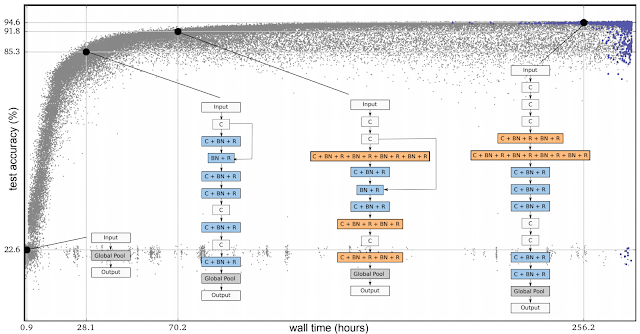
Progress of an evolution experiment. Each dot represents an individual in the population. The four diagrams show examples of discovered architectures. These correspond to the best individual (rightmost; selected by validation accuracy) and three of its ancestors.
The mutations in our first paper are purposefully simple: remove a convolution at random, add a skip connection between arbitrary layers, or change the learning rate, to name a few. This way, the results show the potential of the evolutionary algorithm, as opposed to the quality of the search space. For example, if we had used a single mutation that transforms one of the seed networks into an Inception-ResNet classifier in one step, we would be incorrectly concluding that the algorithm found a good answer. Yet, in that case, all we would have done is hard-coded the final answer into a complex mutation, rigging the outcome. If instead we stick with simple mutations, this cannot happen and evolution is truly doing the job. In the experiment in the figure, simple mutations and the selection process cause the networks to improve over time and reach high test accuracies, even though the test set had never been seen during the process. In this paper, the networks can also inherit their parent's weights. Thus, in addition to evolving the architecture, the population trains its networks while exploring the search space of initial conditions and learning-rate schedules. As a result, the process yields fully trained models with optimized hyperparameters. No expert input is needed after the experiment starts.

In all the above, even though we were minimizing the researcher's participation by having simple initial architectures and intuitive mutations, a good amount of expert knowledge went into the building blocks those architectures were made of. These included important inventions such as convolutions, ReLUs and batch-normalization layers. We were evolving an architecture made up of these components. The term "architecture" is not accidental: this is analogous to constructing a house with high-quality bricks.
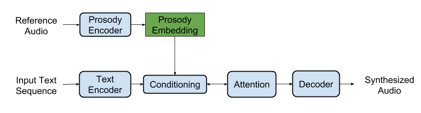
Combining Evolution and Hand Design
After our first paper, we wanted to reduce the search space to something more manageable by giving the algorithm fewer choices to explore. Using our architectural analogy, we removed all the possible ways of making large-scale errors, such as putting the wall above the roof, from the search space. Similarly with neural network architecture searches, by fixing the large-scale structure of the network, we can help the algorithm out. So how to do this? The inception-like modules introduced in Zoph et al. (2017) for the purpose of architecture search proved very powerful. Their idea is to have a deep stack of repeated modules called cells. The stack is fixed but the architecture of the individual modules can change.
The building blocks introduced in Zoph et al. (2017). The diagram on the left is the outer structure of the full neural network, which parses the input data from bottom to top through a stack of repeated cells. The diagram on the right is the inside structure of a cell. The goal is to find a cell that yields an accurate network.
In our second paper, “Regularized Evolution for Image Classifier Architecture Search” (2018), we presented the results of applying evolutionary algorithms to the search space described above. The mutations modify the cell by randomly reconnecting the inputs (the arrows on the right diagram in the figure) or randomly replacing the operations (for example, they can replace the "max 3x3" in the figure, a max-pool operation, with an arbitrary alternative). These mutations are still relatively simple, but the initial conditions are not: the population is now initialized with models that must conform to the outer stack of cells, which was designed by an expert. Even though the cells in these seed models are random, we are no longer starting from simple models, which makes it easier to get to high-quality models in the end. If the evolutionary algorithm is contributing meaningfully, the final networks should be significantly better than the networks we already know can be constructed within this search space. Our paper shows that evolution can indeed find state-of-the-art models that either match or outperform hand-designs.
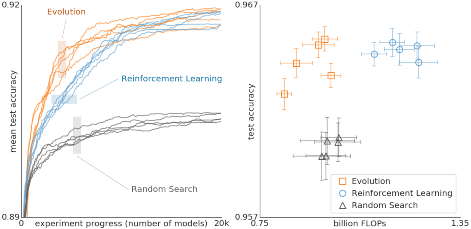
A Controlled Comparison
Even though the mutation/selection evolutionary process is not complicated, maybe an even more straightforward approach (like random search) could have done the same. Other alternatives, though not simpler, also exist in the literature (like reinforcement learning). Because of this, the main purpose of our second paper was to provide a controlled comparison between techniques.
Comparison between evolution, reinforcement learning, and random search for the purposes of architecture search. These experiments were done on the CIFAR-10 dataset, under the same conditions as Zoph et al. (2017), where the search space was originally used with reinforcement learning.
The figure above compares evolution, reinforcement learning, and random search. On the left, each curve represents the progress of an experiment, showing that evolution is faster than reinforcement learning in the earlier stages of the search. This is significant because with less compute power available, the experiments may have to stop early. Moreover evolution is quite robust to changes in the dataset or search space. Overall, the goal of this controlled comparison is to provide the research community with the results of a computationally expensive experiment. In doing so, it is our hope to facilitate architecture searches for everyone by providing a case study of the relationship between the different search algorithms. Note, for example, that the figure above shows that the final models obtained with evolution can reach very high accuracy while using fewer floating-point operations.

One important feature of the evolutionary algorithm we used in our second paper is a form of regularization: instead of letting the worst neural networks die, we remove the oldest ones — regardless of how good they are. This improves robustness to changes in the task being optimized and tends to produce more accurate networks in the end. One reason for this may be that since we didn't allow weight inheritance, all networks must train from scratch. Therefore, this form of regularization selects for networks that remain good when they are re-trained. In other words, because a model can be more accurate just by chance — noise in the training process means even identical architectures may get different accuracy values — only architectures that remain accurate through the generations will survive in the long run, leading to the selection of networks that retrain well. More details of this conjecture can be found in the paper.

The state-of-the-art models we evolved are nicknamed AmoebaNets, and are one of the latest results from our AutoML efforts. All these experiments took a lot of computation — we used hundreds of GPUs/TPUs for days. Much like a single modern computer can outperform thousands of decades-old machines, we hope that in the future these experiments will become household. Here we aimed to provide a glimpse into that future.

Acknowledgements
We would like to thank Alok Aggarwal, Yanping Huang, Andrew Selle, Sherry Moore, Saurabh Saxena, Yutaka Leon Suematsu, Jie Tan, Alex Kurakin, Quoc Le, Barret Zoph, Jon Shlens, Vijay Vasudevan, Vincent Vanhoucke, Megan Kacholia, Jeff Dean, and the rest of the Google Brain team for the collaborations that made this work possible.

Balanced Partitioning and Hierarchical Clustering at Scale


Solving large-scale optimization problems often starts with graph partitioning, which means partitioning the vertices of the graph into clusters to be processed on different machines. The need to make sure that clusters are of near equal size gives rise to the balanced graph partitioning problem. In simple terms, we need to partition the vertices of a given graph into k almost equal clusters, while we minimize the number of edges that are cut by the partition. This NP-hard problem is notoriously difficult in practice because the best approximation algorithms for small instances rely on semidefinite programming which is impractical for larger instances.

This post presents the distributed algorithm we developed which is more applicable to large instances. We introduced this balanced graph-partitioning algorithm in our WSDM 2016 paper, and have applied this approach to several applications within Google. Our more recent NIPS 2017 paper provides more details of the algorithm via a theoretical and empirical study.

Balanced Partitioning via Linear Embedding
Our algorithm first embeds vertices of the graph onto a line, and then processes vertices in a distributed manner guided by the linear embedding order. We examine various ways to find the initial embedding, and apply four different techniques (such as local swaps and dynamic programming) to obtain the final partition. The best initial embedding is based on “affinity clustering”.

Affinity Hierarchical Clustering
Affinity clustering is an agglomerative hierarchical graph clustering based on Borůvka’s classic Maximum-cost Spanning Tree algorithm. As discussed above, this algorithm is a critical part of our balanced partitioning tool. The algorithm starts by placing each vertex in a cluster of its own: v0, v1, and so on. Then, in each iteration, the highest-cost edge out of each cluster is selected in order to induce larger merged clusters: A0, A1, A2, etc. in the first round and B0, B1, etc. in the second round and so on. The set of merges naturally produces a hierarchical clustering, and gives rise to a linear ordering of the leaf vertices (vertices with degree one). The image below demonstrates this, with the numbers at the bottom corresponding to the ordering of the vertices.
Our NIPS’17 paper explains how we run affinity clustering efficiently in the massively parallel computation (MPC) model, in particular using distributed hash tables (DHTs) to significantly reduce running time. This paper also presents a theoretical study of the algorithm. We report clustering results for graphs with tens of trillions of edges, and also observe that affinity clustering empirically beats other clustering algorithms such as k-means in terms of “quality of the clusters”. This video contains a summary of the result and explains how this parallel algorithm may produce higher-quality clusters even compared to a sequential single-linkage agglomerative algorithm.

Comparison to Previous Work
In comparing our algorithm to previous work in (distributed) balanced graph partitioning, we focus on FENNEL, Spinner, METIS, and a recent label propagation-based algorithm. We report results on several public social networks as well as a large private map graph. For a Twitter followership graph, we see a consistent improvement of 15–25% over previous results (Ugander and Backstrom, 2013), and for LiveJournal graph, our algorithm outperforms all the others for all cases except k = 2, where ours is slightly worse than FENNEL's.

The following table presents the fraction of cut edges in the Twitter graph obtained via different algorithms for various values of k, the number of clusters. The numbers given in parentheses denote the size imbalance factor: i.e., the relative difference of the sizes of largest and smallest clusters. Here “Vanilla Affinity Clustering” denotes the first stage of our algorithm where only the hierarchical clustering is built and no further processing is performed on the cuts. Notice that this is already as good as the best previous work (shown in the first two columns below), cutting a smaller fraction of edges while achieving a perfect (and thus better) balance (i.e., 0% imbalance). The last column in the table includes the final result of our algorithm with the post-processing.

k
UB13
(5%)
Vanilla Affinity
Clustering
(0%)
Final Algorithm
(0%)
20
37.0%
38.0%
35.71%
27.50%
40
43.0%
40.0%
40.83%
33.71%
60
46.0%
43.0%
43.03%
36.65%
80
47.5%
44.0%
43.27%
38.65%
100
49.0%
46.0%
45.05%
41.53%

Applications
We apply balanced graph partitioning to multiple applications including Google Maps driving directions, the serving backend for web search, and finding treatment groups for experimental design. For example, in Google Maps the World map graph is stored in several shards. The navigational queries spanning multiple shards are substantially more expensive than those handled within a shard. Using the methods described in our paper, we can reduce 21% of cross-shard queries by increasing the shard imbalance factor from 0% to 10%. As discussed in our paper, live experiments on real traffic show that the number of multi-shard queries from our cut-optimization techniques is 40% less compared to a baseline Hilbert embedding technique. This, in turn, results in less CPU usage in response to queries. In a future blog post, we will talk about application of this work in the web search serving backend, where balanced partitioning helped us design a cache-aware load balancing system that dramatically reduced our cache miss rate.

Acknowledgements
We especially thank Vahab Mirrokni whose guidance and technical contribution were instrumental in developing these algorithms and writing this post. We also thank our other co-authors and colleagues for their contributions: Raimondas Kiveris, Soheil Behnezhad, Mahsa Derakhshan, MohammadTaghi Hajiaghayi, Silvio Lattanzi, Aaron Archer and other members of NYC Algorithms and Optimization research team.

Behind the Motion Photos Technology in Pixel 2


One of the most compelling things about smartphones today is the ability to capture a moment on the fly. With motion photos, a new camera feature available on the Pixel 2 and Pixel 2 XL phones, you no longer have to choose between a photo and a video so every photo you take captures more of the moment. When you take a photo with motion enabled, your phone also records and trims up to 3 seconds of video. Using advanced stabilization built upon technology we pioneered in Motion Stills for Android, these pictures come to life in Google Photos. Let’s take a look behind the technology that makes this possible!
Motion photos on the Pixel 2 in Google Photos. With the camera frozen in place the focus is put directly on the subjects. For more examples, check out this Google Photos album.
Camera Motion Estimation by Combining Hardware and Software
The image and video pair that is captured every time you hit the shutter button is a full resolution JPEG with an embedded 3 second video clip. On the Pixel 2, the video portion also contains motion metadata that is derived from the gyroscope and optical image stabilization (OIS) sensors to aid the trimming and stabilization of the motion photo. By combining software based visual tracking with the motion metadata from the hardware sensors, we built a new hybrid motion estimation for motion photos on the Pixel 2.

Our approach aligns the background more precisely than the technique used in Motion Stills or the purely hardware sensor based approach. Based on Fused Video Stabilization technology, it reduces the artifacts from the visual analysis due to a complex scene with many depth layers or when a foreground object occupies a large portion of the field of view. It also improves the hardware sensor based approach by refining the motion estimation to be more accurate, especially at close distances.
Motion photo as captured (left) and after freezing the camera by combining hardware and software For more comparisons, check out this Google Photos album.
The purely software-based technique we introduced in Motion Stills uses the visual data from the video frames, detecting and tracking features over consecutive frames yielding motion vectors. It then classifies the motion vectors into foreground and background using motion models such as an affine transformation or a homography. However, this classification is not perfect and can be misled, e.g. by a complex scene or dominant foreground.
Feature classification into background (green) and foreground (orange) by using the motion metadata from the hardware sensors of the Pixel 2. Notice how the new approach not only labels the skateboarder accurately as foreground but also the half-pipe that is at roughly the same depth.
For motion photos on Pixel 2 we improved this classification by using the motion metadata derived from the gyroscope and the OIS. This accurately captures the camera motion with respect to the scene at infinity, which one can think of as the background in the distance. However, for pictures taken at closer range, parallax is introduced for scene elements at different depth layers, which is not accounted for by the gyroscope and OIS. Specifically, we mark motion vectors that deviate too much from the motion metadata as foreground. This results in a significantly more accurate classification of foreground and background, which also enables us to use a more complex motion model known as mixture homographies that can account for rolling shutter and undo the distortions it causes.
Background motion estimation in motion photos. By using the motion metadata from Gyro and OIS we are able to accurately classify features from the visual analysis into foreground and background.
Motion Photo Stabilization and Playback
Once we have accurately estimated the background motion for the video, we determine an optimally stable camera path to align the background using linear programming techniques outlined in our earlier posts. Further, we automatically trim the video to remove any accidental motion caused by putting the phone away. All of this processing happens on your phone and produces a small amount of metadata per frame that is used to render the stabilized video in real-time using a GPU shader when you tap the Motion button in Google Photos. In addition, we play the video starting at the exact timestamp as the HDR+ photo, producing a seamless transition from still image to video.
Motion photos stabilize even complex scenes with large foreground motions.
Motion Photo Sharing
Using Google Photos, you can share motion photos with your friends and as videos and GIFs, watch them on the web, or view them on any phone. This is another example of combining hardware, software and Machine Learning to create new features for Pixel 2.

Acknowledgements
Motion photos is a result of a collaboration across several Google Research teams, Google Pixel and Google Photos. We especially want to acknowledge the work of Karthik Raveendran, Suril Shah, Marius Renn, Alex Hong, Radford Juang, Fares Alhassen, Emily Chang, Isaac Reynolds, and Dave Loxton.

Semantic Image Segmentation with DeepLab in Tensorflow


Semantic image segmentation, the task of assigning a semantic label, such as “road”, “sky”, “person”, “dog”, to every pixel in an image enables numerous new applications, such as the synthetic shallow depth-of-field effect shipped in the portrait mode of the Pixel 2 and Pixel 2 XL smartphones and mobile real-time video segmentation. Assigning these semantic labels requires pinpointing the outline of objects, and thus imposes much stricter localization accuracy requirements than other visual entity recognition tasks such as image-level classification or bounding box-level detection.
Today, we are excited to announce the open source release of our latest and best performing semantic image segmentation model, DeepLab-v3+ [1], implemented in Tensorflow. This release includes DeepLab-v3+ models built on top of a powerful convolutional neural network (CNN) backbone architecture [2, 3] for the most accurate results, intended for server-side deployment. As part of this release, we are additionally sharing our Tensorflow model training and evaluation code, as well as models already pre-trained on the Pascal VOC 2012 and Cityscapes benchmark semantic segmentation tasks.

Since the first incarnation of our DeepLab model [4] three years ago, improved CNN feature extractors, better object scale modeling, careful assimilation of contextual information, improved training procedures, and increasingly powerful hardware and software have led to improvements with DeepLab-v2 [5] and DeepLab-v3 [6]. With DeepLab-v3+, we extend DeepLab-v3 by adding a simple yet effective decoder module to refine the segmentation results especially along object boundaries. We further apply the depthwise separable convolution to both atrous spatial pyramid pooling [5, 6] and decoder modules, resulting in a faster and stronger encoder-decoder network for semantic segmentation.
Modern semantic image segmentation systems built on top of convolutional neural networks (CNNs) have reached accuracy levels that were hard to imagine even five years ago, thanks to advances in methods, hardware, and datasets. We hope that publicly sharing our system with the community will make it easier for other groups in academia and industry to reproduce and further improve upon state-of-art systems, train models on new datasets, and envision new applications for this technology.

Acknowledgements
We would like to thank the support and valuable discussions with Iasonas Kokkinos, Kevin Murphy, Alan L. Yuille (co-authors of DeepLab-v1 and -v2), as well as Mark Sandler, Andrew Howard, Menglong Zhu, Chen Sun, Derek Chow, Andre Araujo, Haozhi Qi, Jifeng Dai, and the Google Mobile Vision team.

References
  1. Encoder-Decoder with Atrous Separable Convolution for Semantic Image Segmentation, Liang-Chieh Chen, Yukun Zhu, George Papandreou, Florian Schroff, and Hartwig Adam, arXiv: 1802.02611, 2018.
  2. Xception: Deep Learning with Depthwise Separable Convolutions, François Chollet, Proc. of CVPR, 2017.
  3. Deformable Convolutional Networks — COCO Detection and Segmentation Challenge 2017 Entry, Haozhi Qi, Zheng Zhang, Bin Xiao, Han Hu, Bowen Cheng, Yichen Wei, and Jifeng Dai, ICCV COCO Challenge Workshop, 2017.
  4. Semantic Image Segmentation with Deep Convolutional Nets and Fully Connected CRFs, Liang-Chieh Chen, George Papandreou, Iasonas Kokkinos, Kevin Murphy, and Alan L. Yuille, Proc. of ICLR, 2015.
  5. Deeplab: Semantic Image Segmentation with Deep Convolutional Nets, Atrous Convolution, and Fully Connected CRFs, Liang-Chieh Chen, George Papandreou, Iasonas Kokkinos, Kevin Murphy, and Alan L. Yuille, TPAMI, 2017.
  6. Rethinking Atrous Convolution for Semantic Image Segmentation, Liang-Chieh Chen, George Papandreou, Florian Schroff, and Hartwig Adam, arXiv:1706.05587, 2017.