Author Archives: Research Blog

Announcing TensorFlow 1.0


In just its first year, TensorFlow has helped researchers, engineers, artists, students, and many others make progress with everything from language translation to early detection of skin cancer and preventing blindness in diabetics. We’re excited to see people using TensorFlow in over 6000 open-source repositories online.

Today, as part of the first annual TensorFlow Developer Summit, hosted in Mountain View and livestreamed around the world, we’re announcing TensorFlow 1.0:

It’s faster: TensorFlow 1.0 is incredibly fast! XLA lays the groundwork for even more performance improvements in the future, and tensorflow.org now includes tips & tricks for tuning your models to achieve maximum speed. We’ll soon publish updated implementations of several popular models to show how to take full advantage of TensorFlow 1.0 - including a 7.3x speedup on 8 GPUs for Inception v3 and 58x speedup for distributed Inception v3 training on 64 GPUs!

It’s more flexible: TensorFlow 1.0 introduces a high-level API for TensorFlow, with tf.layers, tf.metrics, and tf.losses modules. We’ve also announced the inclusion of a new tf.keras module that provides full compatibility with Keras, another popular high-level neural networks library.

It’s more production-ready than ever: TensorFlow 1.0 promises Python API stability (details here), making it easier to pick up new features without worrying about breaking your existing code.

Other highlights from TensorFlow 1.0:
  • Python APIs have been changed to resemble NumPy more closely. For this and other backwards-incompatible changes made to support API stability going forward, please use our handy migration guide and conversion script.
  • Experimental APIs for Java and Go
  • Higher-level API modules tf.layers, tf.metrics, and tf.losses - brought over from tf.contrib.learn after incorporating skflow and TF Slim
  • Experimental release of XLA, a domain-specific compiler for TensorFlow graphs, that targets CPUs and GPUs. XLA is rapidly evolving - expect to see more progress in upcoming releases.
  • Introduction of the TensorFlow Debugger (tfdbg), a command-line interface and API for debugging live TensorFlow programs.
  • New Android demos for object detection and localization, and camera-based image stylization.
  • Installation improvements: Python 3 docker images have been added, and TensorFlow’s pip packages are now PyPI compliant. This means TensorFlow can now be installed with a simple invocation of pip install tensorflow.
We’re thrilled to see the pace of development in the TensorFlow community around the world. To hear more about TensorFlow 1.0 and how it’s being used, you can watch the TensorFlow Developer Summit talks on YouTube, covering recent updates from higher-level APIs to TensorFlow on mobile to our new XLA compiler, as well as the exciting ways that TensorFlow is being used:


Click here for a link to the livestream and video playlist (individual talks will be posted online later in the day).

The TensorFlow ecosystem continues to grow with new techniques like Fold for dynamic batching and tools like the Embedding Projector along with updates to our existing tools like TensorFlow Serving. We’re incredibly grateful to the community of contributors, educators, and researchers who have made advances in deep learning available to everyone. We look forward to working with you on forums like GitHub issues, Stack Overflow, @TensorFlow, the [email protected] group and at future events.

On-Device Machine Intelligence


To build the cutting-edge technologies that enable conversational understanding and image recognition, we often apply combinations of machine learning technologies such as deep neural networks and graph-based machine learning. However, the machine learning systems that power most of these applications run in the cloud and are computationally intensive and have significant memory requirements. What if you want machine intelligence to run on your personal phone or smartwatch, or on IoT devices, regardless of whether they are connected to the cloud?

Yesterday, we announced the launch of Android Wear 2.0, along with brand new wearable devices, that will run Google's first entirely “on-device” ML technology for powering smart messaging. This on-device ML system, developed by the Expander research team, enables technologies like Smart Reply to be used for any application, including third-party messaging apps, without ever having to connect with the cloud…so now you can respond to incoming chat messages directly from your watch, with a tap.
The research behind this began last year while our team was developing the machine learning systems that enable conversational understanding capability in Allo and Inbox. The Android Wear team reached out to us and was interested to know whether it would be possible to deploy this Smart Reply technology directly onto a smart device. Because of the limited computing power and memory on smart devices, we quickly realized that it was not possible to do so. Our product manager, Patrick McGregor, realized that this presented a unique challenge and an opportunity for the Expander team to return to the drawing board to design a completely new, lightweight, machine learning architecture — not only to enable Smart Reply on Android Wear, but also to power a wealth of other on-device mobile applications. Together with Tom Rudick, Nathan Beach, and other colleagues from the Android Wear team, we set out to build the new system.

Learning with Projections
A simple strategy to build lightweight conversational models might be to create a small dictionary of common rules (input → reply mappings) on the device and use a naive look-up strategy at inference time. This can work for simple prediction tasks involving a small set of classes using a handful of features (such as binary sentiment classification from text, e.g. “I love this movie” conveys a positive sentiment whereas the sentence “The acting was horrible” is negative). But, it does not scale to complex natural language tasks involving rich vocabularies and the wide language variability observed in chat messages. On the other hand, machine learning models like recurrent neural networks (such as LSTMs), in conjunction with graph learning, have proven to be extremely powerful tools for complex sequence learning in natural language understanding tasks, including Smart Reply. However, compressing such rich models to fit in device memory and produce robust predictions at low computation cost (rapidly on-demand) is extremely challenging. Early experiments with restricting the model to predict only a small handful of replies or using other techniques like quantization or character-level models did not produce useful results.

Instead, we built a different solution for the on-device ML system. We first use a fast, efficient mechanism to group similar incoming messages and project them to similar (“nearby”) bit vector representations. While there are several ways to perform this projection step, such as using word embeddings or encoder networks, we employ a modified version of locality sensitive hashing (LSH) to reduce dimension from millions of unique words to a short, fixed-length sequence of bits. This allows us to compute a projection for an incoming message very fast, on-the-fly, with a small memory footprint on the device since we do not need to store the incoming messages, word embeddings, or even the full model used for training.
Projection step: Similar messages are grouped together and projected to nearby vectors. For example, the messages "hey, how's it going?" and "How's it going buddy?" share similar content and might be projected to the same vector 11100011. Another related message “Howdy, everything going well?” is mapped to a nearby vector 11100110 that differs only in 2 bits.
Next, our system takes the incoming message along with its projections and jointly trains a “message projection model” that learns to predict likely replies using our semi-supervised graph learning framework. The graph learning framework enables training a robust model by combining semantic relationships from multiple sources — message/reply interactions, word/phrase similarity, semantic cluster information — learning useful projection operations that can be mapped to good reply predictions.
Learning step: (Top) Messages along with projections and corresponding replies, if available, are used in a machine learning framework to jointly learn a “message projection model”. (Bottom) The message projection model learns to associate replies with the projections of the corresponding incoming messages. For example, the model projects two different messages “Howdy, everything going well?” and “How’s it going buddy?” (bottom center) to nearby bit vectors and learns to map these to relevant replies (bottom right).
It’s worth noting that while the message projection model can be trained using complex machine learning architectures and the power of the cloud, as described above, the model itself resides and performs inference completely on device. Apps running on the device can pass a user’s incoming messages and receive reply predictions from the on-device model without data leaving the device. The model can also be adapted to cater to the user’s writing style and individual preferences to provide a personalized experience.
Inference step: The model applies the learned projections to an incoming message (or sequence of messages) and suggests relevant and diverse replies. Inference is performed on the device, allowing the model to adapt to user data and personal writing styles.
To get the on-device system to work out of the box, we had to make a few additional improvements such as optimizing for speeding up computations on device and generating rich, diverse replies from the model. We will have a forthcoming scientific publication that describes the on-device machine learning work in more detail.

Converse from Your Wrist
When we embarked on our journey to build this technology from scratch, we weren’t sure if the predictions would be useful or of sufficient quality. We’re quite surprised and excited about how well it works even on Android wearable devices with very limited computation and memory resources. We look forward to continuing to improve the models to provide users with more delightful conversational experiences, and we will be leveraging this on-device ML platform to enable completely new applications in the months to come.

You can now use this feature to respond to your messages directly from your Google watches or any watch that runs Android Wear 2.0. It is already enabled on Google Hangouts, Google Messenger, and many third-party messaging apps. We also provide an API for developers of third-party Wear apps.

Acknowledgements
On behalf of the Google Expander team, I would also like to thank the following people who helped make this technology a success: Andrei Broder, Andrew Tomkins, David Singleton, Mirko Ranieri, Robin Dua and Yicheng Fan.

Announcing TensorFlow Fold: Deep Learning With Dynamic Computation Graphs


In much of machine learning, data used for training and inference undergoes a preprocessing step, where multiple inputs (such as images) are scaled to the same dimensions and stacked into batches. This lets high-performance deep learning libraries like TensorFlow run the same computation graph across all the inputs in the batch in parallel. Batching exploits the SIMD capabilities of modern GPUs and multi-core CPUs to speed up execution. However, there are many problem domains where the size and structure of the input data varies, such as parse trees in natural language understanding, abstract syntax trees in source code, DOM trees for web pages and more. In these cases, the different inputs have different computation graphs that don't naturally batch together, resulting in poor processor, memory, and cache utilization.

Today we are releasing TensorFlow Fold to address these challenges. TensorFlow Fold makes it easy to implement deep-learning models that operate over data of varying size and structure. Furthermore, TensorFlow Fold brings the benefits of batching to such models, resulting in a speedup of more than 10x on CPU, and more than 100x on GPU, over alternative implementations. This is made possible by dynamic batching, introduced in our paper Deep Learning with Dynamic Computation Graphs.
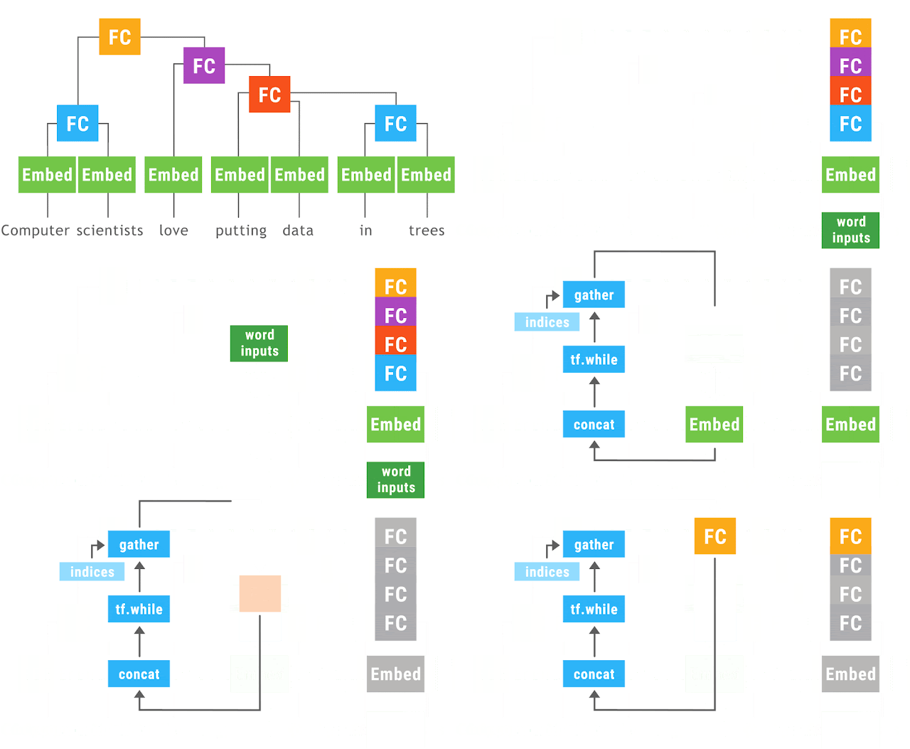
This animation shows a recursive neural network run with dynamic batching. Operations with the same color are batched together, which lets TensorFlow run them faster. The Embed operation converts words to vector representations. The fully connected (FC) operation combines word vectors to form vector representations of phrases. The output of the network is a vector representation of an entire sentence. Although only a single parse tree of a sentence is shown, the same network can run, and batch together operations, over multiple parse trees of arbitrary shapes and sizes.
The TensorFlow Fold library will initially build a separate computation graph from each input.
Because the individual inputs may have different sizes and structures, the computation graphs may as well. Dynamic batching then automatically combines these graphs to take advantage of opportunities for batching, both within and across inputs, and inserts additional instructions to move data between the batched operations (see our paper for technical details).

To learn more, head over to our github site. We hope that TensorFlow Fold will be useful for researchers and practitioners implementing neural networks with dynamic computation graphs in TensorFlow.

Acknowledgements
This work was done under the supervision of Peter Norvig.

Advancing Research on Video Understanding with the YouTube-BoundingBoxes Dataset


One of the most challenging research areas in machine learning today is enabling computers to understand what a scene is about. For example, while humans know that a ball that disappears behind a wall only to reappear a moment later is very likely the same object, this is not at all obvious to an algorithm. Understanding this requires not only a global picture of what objects are contained in each frame of a video, but also where those objects are located within the frame and their locations over time. Just last year we published YouTube-8M, a dataset consisting of automatically labelled YouTube videos. And while this helps further progress in the field, it is only one piece to the puzzle.

Today, in order to facilitate progress in video understanding research, we are introducing YouTube-BoundingBoxes, a dataset consisting of 5 million bounding boxes spanning 23 object categories, densely labeling segments from 210,000 YouTube videos. To date, this is the largest manually annotated video dataset containing bounding boxes, which track objects in temporally contiguous frames. The dataset is designed to be large enough to train large-scale models, and be representative of videos captured in natural settings. Importantly, the human-labelled annotations contain objects as they appear in the real world with partial occlusions, motion blur and natural lighting.
Summary of dataset statistics. Bar Chart: Relative number of detections in existing image (red) and video (blue) data sets. The YouTube BoundingBoxes dataset (YT-BB) is at the bottom, is at the bottom. Table: The three columns are counts for: classification annotations, bounding boxes, and unique videos with bounding boxes. Full details on the dataset can be found in the preprint.
A key feature of this dataset is that bounding box annotations are provided for entire video segments. These bounding box annotations may be used to train models that explicitly leverage this temporal information to identify, localize and track objects over time. In a video, individual annotated objects might become entirely occluded and later return in subsequent frames. These annotations of individual objects are sometimes not recognizable from individual frames, but can be understood and recognized in the context of the video if the objects are localized and tracked accurately.
Three video segments, sampled at 1 frame per second. The final frame of each example shows how it is visually challenging to recognize the bounded object, due to blur or occlusion (train example, blue arrow). However, temporally-related frames, where the object has been more clearly identified, can allow object classes to be inferred. Note how only visible parts are included in the box: the orange arrow in the bear example (middle row) points to the hidden head. The dog example illustrates tight bounding boxes that track the tail (orange arrows) and foot (blue arrows). The airplane example illustrates how partial objects are annotated (first frame) tracked across changes in perspective, occlusions and camera cuts.
We hope that this dataset might ultimately aid the computer vision and machine learning community and lead to new methods for analyzing and understanding real world vision problems. You can learn more about the dataset in this associated preprint.

Acknowledgements
The work was greatly helped along by Xin Pan and Thomas Silva, as well as support and advice from Manfred Georg, Sami Abu-El-Haija, Susanna Ricco and George Toderici.

Using Machine Learning to predict parking difficulty


"When Solomon said there was a time and a place for everything he had not encountered the problem of parking his automobile." -Bob Edwards, Broadcast Journalist

Much of driving is spent either stuck in traffic or looking for parking. With products like Google Maps and Waze, it is our long-standing goal to help people navigate the roads easily and efficiently. But until now, there wasn’t a tool to address the all-too-common parking woes.

Last week, we launched a new feature for Google Maps for Android across 25 US cities that offers predictions about parking difficulty close to your destination so you can plan accordingly. Providing this feature required addressing some significant challenges:
  • Parking availability is highly variable, based on factors like the time, day of week, weather, special events, holidays, and so on. Compounding the problem, there is almost no real time information about free parking spots.
  • Even in areas with internet-connected parking meters providing information on availability, this data doesn’t account for those who park illegally, park with a permit, or depart early from still-paid meters.
  • Roads form a mostly-planar graph, but parking structures may be more complex, with traffic flows across many levels, possibly with different layouts.
  • Both the supply and the demand for parking are in constant flux, so even the best system is at risk of being outdated as soon as it’s built.
To face these challenges, we used a unique combination of crowdsourcing and machine learning (ML) to build a system that can provide you with parking difficulty information for your destination, and even help you decide what mode of travel to take — in a pre-launch experiment, we saw a significant increase in clicks on the transit travel mode button, indicating that users with additional knowledge of parking difficulty were more likely to consider public transit rather than driving.

Three technical pieces were required to build the algorithms behind the parking difficulty feature: good ground truth data from crowdsourcing, an appropriate ML model and a robust set of features to train the model on.

Ground Truth Data
Gathering high-quality ground truth data is often a key challenge in building any ML solution. We began by asking individuals at a diverse set of locations and times if they found the parking difficult. But we learned that answers to subjective questions like this produces inconsistent results - for a given location and time, one person may answer that it was “easy” to find parking while another found it “difficult.” Switching to objective questions like “How long did it it take to find parking?” led to an increase in answer confidence, enabling us to crowdsource a high-quality set of ground truth data with over 100K responses.

Model Features
With this data available, we began to determine features we could train a model on. Fortunately, we were able to turn to the wisdom of the crowd, and utilize anonymous aggregated information from users who opt to share their location data, which already is a vital source of information for estimates of live traffic or popular times and visit durations.

We quickly discovered that even with this data, some unique challenges remain. For example, our system shouldn’t be fooled into thinking parking is plentiful if someone is parking in a gated or private lot. Users arriving by taxi might look like a sign of abundant parking at the front door, and similarly, public-transit users might seem to park at bus stops. These false positives, and many others, all have the potential to mislead an ML system.

So we needed more robust aggregate features. Perhaps not surprisingly, the inspiration for one of these features came from our own backyard in downtown Mountain View. If Google navigation observes many users circling downtown Mountain View during lunchtime along trajectories like this one, it strongly suggests that parking might be difficult:
Our team thought about how to recognize this “fingerprint” of difficult parking as a feature to train on. In this case, we aggregate the difference between when a user should have arrived at a destination if they simply drove to the front door, versus when they actually arrived, taking into account circling, parking, and walking. If many users show a large gap between these two times, we expect this to be a useful signal that parking is difficult.

From there, we continued to develop more features that took into account, for any particular destination, dispersion of parking locations, time-of-day and date dependence of parking (e.g. what if users park close to a destination in the early morning, but further away at busier hours?), historical parking data and more. In the end, we decided on roughly twenty different features along these lines for our model. Then it was time to tune the model performance.

Model Selection & Training
We decided to use a standard logistic regression ML model for this feature, for a few different reasons. First, the behavior of logistic regression is well understood, and it tends to be resilient to noise in the training data; this is a useful property when the data comes from crowdsourcing a complicated response variable like difficulty of parking. Second, it’s natural to interpret the output of these models as the probability that parking will be difficult, which we can then map into descriptive terms like “Limited parking” or “Easy.” Third, it’s easy to understand the influence of each specific feature, which makes it easier to verify that the model is behaving reasonably. For example, when we started the training process, many of us thought that the “fingerprint” feature described above would be the “silver bullet” that would crack the problem for us. We were surprised to note that this wasn’t the case at all — in fact, it was features based on the dispersion of parking locations that turned out to be one of the most powerful predictors of parking difficulty.

Results
With our model in hand, we were able to generate an estimate for difficulty of parking at any place and time. The figure below gives a few examples of the output of our system, which is then used to provide parking difficulty estimates for a given destination. Parking on Monday mornings, for instance, is difficult throughout the city, especially in the busiest financial and retail areas. On Saturday night, things are busy again, but now predominantly in the areas with restaurants and attractions.
Output of our parking difficulty model in the Financial District and Union Square areas of San Francisco. Red denotes a higher confidence that parking is difficult. Top row: a typical Monday at ~8am (left) and ~9pm (right). Bottom row: the same times but on a typical Saturday.
We’re excited about the opportunities to continue to improve the model quality based on user feedback. If we are able to better understand parking difficulty, we will be able to develop new and smarter forms of parking assistance — we’re very excited about future applications of ML to help make transportation more enjoyable!

App Discovery With Google Play, Part 3: Machine Learning to Fight Spam and Abuse at Scale


In Part 1 and Part 2 of this series on app discovery, we discussed using machine learning to gain a deeper understanding of the topics associated with an app, and a deep learning framework to provide personalized recommendations. In this post, we discuss a machine learning approach to fight spam and abuse on apps section of the Google Play Store, making it a safe and trusted app platform for more than a billion Android users.

With apps becoming an increasingly important part of people’s professional and personal lives, we realize that it is critical to make sure that 1) the apps found on Google Play are safe, and 2) the information presented to you about the apps is both authentic and unbiased. With more than 1 million apps in our catalog, and a significant number of new apps introduced everyday, we needed to develop scalable methods to identify bad actors accurately and swiftly. To tackle this problem, we take a two-pronged approach, both employing various machine learning techniques to help fight against spam and abuse at scale.

Identifying and blocking ‘bad’ apps from entering Google Play platform

As mentioned in Google Play Developer Policy, we don’t allow listing of malicious, offensive, or illegal apps. Despite such policy, there are always a small number of bad actors who attempt to publish apps that prey on users. Finding the apps that violate our policy among the vast app catalog is not a trivial problem, especially when there are tens of thousands of apps being submitted each day. This is why we embraced machine learning techniques in assessing policy violations and potential risks an app may pose to its potential users.

We use various techniques such as text analysis with word embedding with large probabilistic networks, image understanding with Google Brain, and static and dynamic analysis of the APK binary. These individual techniques are aimed to detect specific violations (e.g., restricted content, privacy and security, intellectual property, user deception), in a more systematic and reliable way compared to manual reviews. Apps that are flagged by our algorithms either gets sent back to the developers for addressing the detected issues, or are ‘quarantined’ until we can verify its safety and/or clears it of potential violations. Because of this app review process combining analyses by human experts and algorithms, developers can take necessary actions (e.g., iterate or publish) within a few hours of app submission.
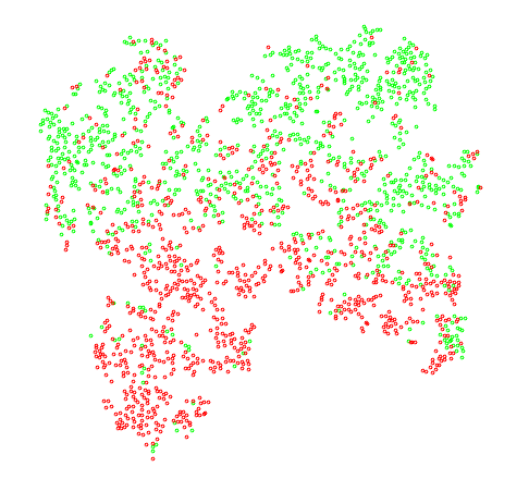
Visualization of word embedding of samples of offensive content policy violating apps (red dots) and policy compliant apps (green dots), visualized with t-SNE (t-Distributed Stochastic Neighbor Embedding).

Preventing manipulation of app ratings and rankings

While an app may itself be legitimate, some bad actors may attempt to create fake engagements in order to manipulate an app’s ratings and rankings. In order to provide our users with an accurate reflection of the app’s perceived quality, we work to nullify these attempts. However, as we place countermeasures against these efforts, the actors behind the manipulation attempts change and adapt their behaviors to bypass our countermeasures thereby presenting us with an adversarial problem.

As such, instead of using a conventional supervised learning approach (as we did in the ‘Part 1’ or ‘Part 2’ of this series, which are more ‘stationary’ problems), we needed to develop a repeatable process that allowed us the same (if not more) agility that bad actors have. We achieved this by using a hybrid strategy that utilizes unsupervised learning techniques to generate training data which in turn feeds into a model built on traditional supervised learning techniques.

Utilizing data on interactions, transactions, and behaviors occurring on the Google Play platform, we apply anomaly detection techniques to identify apps that are targeted by fake engagements. For example, a suspected app may have all its engagement originating from a single data center, whereas an app with organic engagement will have its engagement originating from a healthy distribution of sources.

We then use these apps to isolate actors who collude or orchestrate to manipulate ratings and rankings, who in turn are used as training data to build a model that identifies similar actors. This model, built using supervised learning techniques, is then used to expand coverage and nullify fake engagements across Google Play Apps platform.
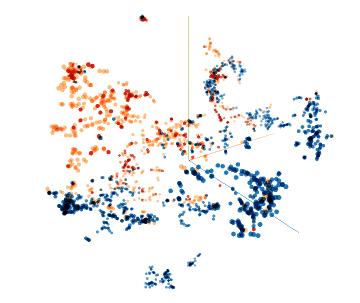
A visualization of how a model trained on known bad actors (red) expands coverage to detect similar bad actors (orange) while ignoring organic users (blue).

We strive to make Google Play the best platform for both developers and users, by enabling fast publication while not compromising user safety. The machine learning capabilities mentioned above helped us achieve both, and we’ll continue to innovate on these techniques to ensure we keep our users safe from spam and abuse.

Acknowledgements
This work was done in close collaboration with Yang Zhang, Zhikun Wang, Gengxin Miao, Liam MacDermed, Dev Manuel, Daniel Peddity, Yi Li, Kazushi Nagayama, Sid Chahar, and Xinyu Cheng.

Facilitating the discovery of public datasets


There are many hundreds of data repositories on the Web, providing access to tens of thousands—or millions—of datasets. National and regional governments, scientific publishers and consortia, commercial data providers, and others publish data for fields ranging from social science to life science to high-energy physics to climate science and more. Access to this data is critical to facilitating reproducibility of research results, enabling scientists to build on others’ work, and providing data journalists easier access to information and its provenance. For these reasons, many publishers and funding agencies now require that scientists make their research data available publicly.

However, due to the volume of data repositories available on the Web, it can be extremely difficult to determine not only where is the dataset that has the information that you are looking for, but also the veracity or provenance of that information. Yet, there is no reason why searching for datasets shouldn’t be as easy as searching for recipes, or jobs, or movies. These types of searches are often open-ended ones, where some structure over the search space makes the exploration and serendipitous discovery possible.

To provide better discovery and rich content for books, movies, events, recipes, reviews and a number of other content categories with Google Search, we rely on structured data that content providers embed in their sites using schema.org vocabulary. To facilitate similar capabilities for datasets, we have recently published new guidelines to help data providers describe their datasets in a structured way, enabling Google and others to link this structured metadata with information describing locations, scientific publications, or even Knowledge Graph, facilitating data discovery for others. We hope that this metadata will help us improve the discovery and reuse of public datasets on the Web for everybody.

The schema.org approach for describing datasets is based on an effort recently standardized at W3C (the Data Catalog Vocabulary), which we expect will be a foundation for future elaborations and improvements to dataset description. While these industry discussions are evolving, we are confident that the standards that already exist today provide a solid basis for building a data ecosystem.

Technical Challenges
While we have released the guidelines on publishing the metadata, many technical challenges remain before search for data becomes as seamless as we feel it should be. These challenges include:
  • Defining more consistently what constitutes a dataset: For example, is a single table a dataset? What about a collection of related tables? What about a protein sequence? A set of images? An API that provides access to data? We hope that a better understanding of what a dataset is will emerge as we gain more experience with how data providers define, describe, and use data.
  • Identifying datasets: Ideally, datasets should have permanent identifiers conforming to some well known scheme that enables us to identify them uniquely, but often they don’t. Is a URL for the metadata page a good identifier? Can there be multiple identifiers? Is there a primary one?
  • Relating datasets to each other: When are two records describing a dataset “the same” (for instance, if one repository copies metadata from another )? What if an aggregator provides more metadata about the same dataset or cleans the data in some useful way? We are working on clarifying and defining these relationships, but it is likely that consumers of metadata will have to assume that many data providers are using these predicates imprecisely and need to be tolerant of that.
  • Propagating metadata between related datasets: How much of the metadata can we propagate among related datasets? For instance, we can probably propagate provenance information from a composite dataset to the datasets that it contains. But how much does the metadata “degrade” with such propagation? We expect the answer to be different depending on the application: metadata for search applications may be less precise than, say, for data integration.
  • Describing content of datasets: How much of the dataset content should we describe to enable support for queries similar to those used in Explore for Docs, Sheets and Slides, or other exploration and reuse of the content of the datasets (where license terms allow, of course)? How can we efficiently use content descriptions that providers already describe in a declarative way using W3C standards for describing semantics of Web resources and linked data?
In addition to the technical and social challenges that we’ve just listed, many remaining research challenges touch on longer term open-ended research: Many datasets are described in unstructured way, in captions, figures, and tables of scientific papers and other documents. We can build on other promising efforts to extract this metadata. While we have a reasonable handle on ranking in the content of Web search, ranking datasets is often a challenging problem: we don’t know yet if the same signals that work for ranking Web pages will work equally well for ranking datasets. In the cases where the dataset content is public and available, we may be able to extract additional semantics about the dataset, for example, by learning the types of values in different fields. Indeed, can we understand the content enough to enable data integration and discovery of related resources?

A Call to Action
As any ecosystem, a data ecosystem will thrive only if a variety of players contribute to it:
  • For data providers, both individual providers and data repositories: publishing structured metadata using schema.org, DCAT, CSVW, and other community standards will make this metadata available for others to discover and use.
  • For data consumers (from scientists to data journalists and more): citing data properly, much as we cite scientific publications (see, for example, a recently proposed approach).
  • For developers: to contribute to expanding schema.org metadata for datasets, providing domain-specific vocabularies, as well as working on tools and applications that consume this rich metadata.
Our ultimate goal is to help foster an ecosystem for publishing, consuming and discovering datasets. As such, this ecosystem would include data publishers, aggregators (in the form of large data repositories that provide additional value by cleaning and reconciling metadata), search engines that enable data discovery of the data, and, most important, data consumers.

A Large Corpus for Supervised Word-Sense Disambiguation


Understanding the various meanings of a particular word in text is key to understanding language. For example, in the sentence “he will receive stock in the reorganized company”, we know that “stock” refers to “the capital raised by a business or corporation through the issue and subscription of shares” as defined in the New Oxford American Dictionary (NOAD), based on the context. However, there are more than 10 other definitions for “stock” in NOAD, ranging from “goods in a store”to “a medieval device for punishment”. For a computer algorithm, distinguishing between these meanings is so difficult that it has been described as “AI-complete” in the past (Navigli, 2009; Ide and Veronis 1998; Mallery 1988).

In order to help further progress on this challenge, we’re happy to announce the release of word-sense annotations on the popular MASC and SemCor datasets, manually annotated with senses from the NOAD. We’re also releasing mappings from the NOAD senses to English Wordnet, which is more commonly used by the research community. This is one of the largest releases of fully sense-annotated English corpora.

Supervised Word-Sense Disambiguation
Humans distinguish between meanings of words in text easily because we have access to an enormous amount of common-sense knowledge about how the world works, and how this connects to language. For an example of the difficulty, “[stock] in a business” implies the financial sense, but “[stock] in a bodega” is more likely to refer to goods on the shelves of a store, even though a bodega is a kind of business. Acquiring sufficient knowledge in a form that a machine can use, and then applying it to understanding the words in text, is a challenge.

Supervised word-sense disambiguation (WSD) is the problem of building a machine-learned system using human-labeled data that can assign a dictionary sense to all words used in text (in contrast to entity disambiguation, which focuses on nouns, mostly proper). Building a supervised model that performs better than just assigning the most frequent sense of a word without considering the surrounding text is difficult, but supervised models can perform well when supplied with significant amounts of training data. (Navigli, 2009)

By releasing this dataset, it is our hope that the research community will be able to further the advance of algorithms that allow machines to understand language better, allowing applications such as:
  • Facilitating the automatic construction of databases from text in order to answer questions and connect knowledge in documents. For example, understanding that a “hemi engine” is a kind of automotive machinery, and a “locomotive engine” is a kind of train, or that “Kanye West is a star” implies that he is a celebrity, but “Sirius is a star” implies that it is an astronomical object.
  • Disambiguating words in queries, so that results for “date palm” and “date night” or “web spam” and “spam recipe” can have distinct interpretations for different senses, and documents returned from a query have the same meaning that is implied by the query.
Manual Annotation
In the manually labeled data sets that we are releasing, each sense annotation is labeled by five raters. To ensure high quality of the sense annotation, raters are first trained with gold annotations, which were labeled by experienced linguists in a separate pilot study before the annotation task. The figure below shows an example of a rater’s work page in our annotation tool.

The left side of the page lists all candidate dictionary senses (in this case, the word “general”). Example sentences from the dictionary are also provided. The to-be-annotated words, highlighted within a sentence, are shown on the right side of the work page. Besides linking a dictionary sense to a word, raters could also label one of the three exceptions: (1) The word is a typo (2) None of the above and (3) I can’t decide. Raters could also check whether the word usage is a metaphor and leave comments.

The sense annotation task used for this data release achieves an inter-rater reliability score of 0.869 using Krippendorff's alpha (α >= 0.67 is considered an acceptable level of reproducibility, and α >= 0.80 is considered a highly reproducible result) (Krippendorff, 2004). Annotation counts are listed below.

Total
noun
verb
adjective
adverb
SemCor
115k
38k
57k
11.6k
8.6k
MASC
133k
50k
12.7k
13.6k
4.2k

Wordnet Mappings
We’ve also included two sets of mappings from NOAD to Wordnet. A smaller set of 2200 words was manually mapped in a process similar to the sense annotations described above, and a larger set was created algorithmically. Together, these mappings allow for resources in Wordnet to be applied to this NOAD corpus, and for systems built using Wordnet to be evaluated using this corpus.

You can learn more about our full research results on this corpus using LSTM-based language models and semi-supervised learning in “Semi-supervised Word Sense Disambiguation with Neural Models”.

Acknowledgements
The datasets were built with help from Eric Altendorf, Heng Chen, Jutta Degener, Ryan Doherty, David Huynh, Ji Li, Julian Richardson and Binbin Ruan.

The Google Brain team — Looking Back on 2016


The Google Brain team's long-term goal is to create more intelligent software and systems that improve people's lives, which we pursue through both pure and applied research in a variety of different domains. And while this is obviously a long-term goal, we would like to take a step back and look at some of the progress our team has made over the past year, and share what we feel may be in store for 2017.

Research Publications
One important way in which we assess the quality of our research is through publications in top tier international machine learning venues like ICML, NIPS, and ICLR. Last year our team had a total of 27 accepted papers at these venues, covering a wide ranging set of topics including program synthesis, knowledge transfer from one network to another, distributed training of machine learning models, generative models for language, unsupervised learning for robotics, automated theorem proving, better theoretical understanding of neural networks, algorithms for improved reinforcement learning, and many others. We also had numerous other papers accepted at conferences in fields such as natural language processing (ACL, CoNNL), speech (ICASSP), vision (CVPR), robotics (ISER), and computer systems (OSDI). Our group has also submitted 34 papers to the upcoming ICLR 2017, a top venue for cutting-edge deep learning research. You can learn more about our work in our list of papers, here.

Natural Language Understanding
Allowing computers to better understand human language is one key area for our research. In late 2014, three Brain team researchers published a paper on Sequence to Sequence Learning with Neural Networks, and demonstrated that the approach could be used for machine translation. In 2015, we showed that this this approach could also be used for generating captions for images, parsing sentences, and solving computational geometry problems. In 2016, this previous research (plus many enhancements) culminated in Brain team members worked closely with members of the Google Translate team to wholly replace the translation algorithms powering Google Translate with a completely end-to-end learned system (research paper). This new system closed the gap between the old system and human quality translations by up to 85% for some language pairs. A few weeks later, we showed how the system could do “zero-shot translation”, learning to translate between languages for which it had never seen example sentence pairs (research paper). This system is now deployed on the production Google Translate service for a growing number of language pairs, giving our users higher quality translations and allowing people to communicate more effectively across language barriers. Gideon Lewis-Kraus documented this translation effort (along with the history of deep learning and the history of the Google Brain team) in “The Great A.I. Awakening”, an in-depth article that appeared in The NY Times Magazine in December, 2016.

Robotics
Traditional robotics control algorithms are carefully and painstakingly hand-programmed, and therefore embodying robots with new capabilities is often a very laborious process. We believe that having robots automatically learn to acquire new skills through machine learning is a better approach. Last year, we collaborated with researchers at [X] to demonstrate how robotic arms could learn hand-eye coordination, pooling their experiences to teach themselves more quickly (research paper). Our robots made about 800,000 grasping attempts during this research. Later in the year, we explored three possible ways for robots to learn new skills, through reinforcement learning, through their own interaction with objects, and through human demonstrations. We’re continuing to build on this work in our goals for making robots that are able to flexibly and readily learn new tasks and operate in messy, real-world environments. To help other robotics researchers, we have made multiple robotics datasets publicly available.

Healthcare
We are excited by the potential to use machine learning to augment the abilities of doctors and healthcare practitioners. As just one example of the possibilities, in a paper published in the Journal of the American Medical Association (JAMA), we demonstrated that a machine-learning driven system for diagnosing diabetic retinopathy from a retinal image could perform on-par with board-certified ophthalmologists. With more than 400 million people at risk for blindness if early symptoms of diabetic retinopathy go undetected, but too few ophthalmologists to perform the necessary screening in many countries, this technology could help ensure that more people receive the proper screening. We are also doing work in other medical imaging domains, as well as investigating the use of machine learning for other kinds of medical prediction tasks. We believe that machine learning can improve the quality and efficiency of the healthcare experience for doctors and patients, and we’ll have more to say about our work in this area in 2017.

Music and Art Generation
Technology has always helped define how people create and share media — consider the printing press, film or the electric guitar. Last year we started a project called Magenta to explore the intersection of art and machine intelligence, and the potential of using machine learning systems to augment human creativity. Starting with music and image generation and moving to areas like text generation and VR, Magenta is advancing the state-of-the-art in generative models for content creation. We’ve helped to organize a one-day symposium on these topics and supported an art exhibition of machine generated art. We’ve explored a variety of topics in music generation and artistic style transfer, and our jam session demo won the Best Demo Award at NIPS 2016.

AI Safety and Fairness
As we develop more powerful and sophisticated AI systems and deploy them in a wider variety of real-world settings, we want to ensure that these systems are both safe and fair, and we also want to build tools to help humans better understand the output they produce. In the area of AI safety, in a cross-institutional collaboration with researchers at Stanford, Berkeley, and OpenAI, we published a white paper on Concrete Problems in AI Safety (see the blog post here). The paper outlines some specific problems and areas where we believe there is real and foundational research to be done in the area of AI safety. One aspect of safety on which we are making progress is the protection of the privacy of training data, obtaining differential privacy guarantees, most recently via knowledge transfer techniques. In addition to safety, as we start to rely on AI systems to make more complex and sophisticated decisions, we want to ensure that those decisions are fair. In a paper on equality of opportunity in supervised learning (see the blog post here), we showed how to optimally adjust any trained predictor to prevent one particular formal notion of discrimination, and the paper illustrated this with a case study based on FICO credit scores. To make this work more accessible, we also created a visualization to help illustrate and interactively explore the concepts from the paper.

TensorFlow
In November 2015, we open-sourced an initial version of TensorFlow so that the rest of the machine learning community could benefit from it and we could all collaborate to jointly improve it. In 2016, TensorFlow became the most popular machine learning project on GitHub, with over 10,000 commits by more than 570 people. TensorFlow’s repository of models has grown with contributions from the community, and there are also more than 5000 TensorFlow-related repositories listed on GitHub alone! Furthermore, TensorFlow has been widely adopted by well-known research groups and large companies including DeepMind, and applied towards or some unusual applications like finding sea cows Down Under and sorting cucumbers in Japan.

We’ve made numerous performance improvements, added support for distributed training, brought TensorFlow to iOS, Raspberry Pi and Windows, and integrated TensorFlow with widely-used big data infrastructure. We’ve extended TensorBoard, TensorFlow’s visualization system with improved tools for visualizing computation graphs and embeddings. We’ve also made TensorFlow accessible from Go, Rust and Haskell, released state-of-the-art image classification models, Wide and Deep and answered thousands of questions on GitHub, StackOverflow and the TensorFlow mailing list along the way. TensorFlow Serving simplifies the process of serving TensorFlow models in production, and for those working in the cloud, Google Cloud Machine Learning offers TensorFlow as a managed service.

Last November, we celebrated TensorFlow’s one year anniversary as an open-source project, and presented a paper on the computer systems aspects of TensorFlow at OSDI, one of the premier computer systems research conferences. In collaboration with our colleagues in the compiler team at Google we’ve also been hard at work on a backend compiler for TensorFlow called XLA, an alpha version of which was recently added to the open-source release.

Machine Learning Community Involvement
We also strive to educate and mentor people in how to do machine learning and how to conduct research in this field. Last January, Vincent Vanhoucke, one of the research leads in the Brain team, developed and worked with Udacity to make available a free online deep learning course (blog announcement). We also put together TensorFlow Playground, a fun and interactive system to help people better understand and visualize how very simple neural networks learn to accomplish tasks.

In June we welcomed our first class of 27 Google Brain Residents, selected from more than 2200 applicants, and in seven months they have already conducted significantly original research, helping to author 21 research papers. In August, many Brain team members took part in a Google Brain team Reddit AMA (Ask Me Anything) on r/MachineLearning to answer the community’s questions about machine learning and our team. Throughout the year, we also hosted 46 student interns (mostly Ph.D. students) in our group to conduct research and work with our team members.

Spreading Machine Learning within Google
In addition to the public-facing activities outlined above, we have continued to work within Google to spread machine learning expertise and awareness throughout our many product teams, and to ensure that the company as a whole is well positioned to take advantage of any new machine learning research that emerges. As one example, we worked closely with our platforms team to provide specifications and high level goals for Google’s Tensor Processing Unit (TPU), a custom machine learning accelerator ASIC that was discussed at Google I/O. This custom chip provides an order of magnitude improvement for machine learning workloads, and is heavily used throughout our products, including for RankBrain, for the recently launched Neural Machine Translation system, and for the AlphaGo match against Lee Sedol in Korea last March.

All in all, 2016 was an exciting year for the Google Brain team and our many collaborators and colleagues both within and outside of Google, and we look forward to our machine learning research having significant impact in 2017!

Google Brain Residency Program – 7 months in and looking ahead


“Beyond being incredibly instructive, the Google Brain Residency program has been a truly affirming experience. Working alongside people who truly love what they do--and are eager to help you develop your own passion--has vastly increased my confidence in my interests, my ability to explore them, and my plans for the near future.”
-Akosua Busia, B.S. Mathematical and Computational Science, Stanford University ‘16
2016 Google Brain Resident

In October 2015 we launched the Google Brain Residency, a 12-month program focused on jumpstarting a career for those interested in machine learning and deep learning research. This program is an opportunity to get hands on experience using the state-of-the-art infrastructure available at Google, and offers the chance to work alongside top researchers within the Google Brain team.

Our first group of residents arrived in June 2016, working with researchers on problems at the forefront of machine learning. The wide array of topics studied by residents reflects the diversity of the residents themselves — some come to the program as new graduates with degrees ranging from BAs to Ph.Ds in computer science to physics and mathematics to biology and neuroscience, while other residents come with years of industry experience under their belts. They all have come with a passion for learning how to conduct machine learning research.

The breadth of research being done by the Google Brain Team along with resident-mentorship pairing flexibility ensures that residents with interests in machine learning algorithms and reinforcement learning, natural language understanding, robotics, neuroscience, genetics and more, are able to find good mentors to help them pursue their ideas and publish interesting work. And just seven months into the program, the Residents are already making an impact in the research field.

To date, Google Brain Residents have submitted a total of 21 papers to leading machine learning conferences, spanning topics from enhancing low resolution images to building neural networks that in turn design novel, task specific neural network architectures. Of those 21 papers, 5 were accepted in the recent BayLearn Conference (two of which, “Mean Field Neural Networks” and “Regularizing Neural Networks by Penalizing Their Output Distribution’’, were presented in oral sessions), 2 were accepted in the NIPS 2016 Adversarial Training workshop, and another in ISMIR 2016 (see the full list of papers, including the 14 submissions to ICLR 2017, after the figures below).
An LSTM Cell (Left) and a state of the art RNN Cell found using a neural network (Right). This is an example of a novel architecture found using the approach presented in “Neural Architecture Search with Reinforcement Learning” (B. Zoph and Q. V. Le, submitted to ICLR 2017). This paper uses a neural network to generate novel RNN cell architectures that outperform the widely used LSTM on a variety of different tasks.
The training accuracy for neural networks, colored from black (random chance) to red (high accuracy). Overlaid in white dashed lines are the theoretical predictions showing the boundary between trainable and untrainable networks. (a) Networks with no dropout. (b)-(d) Networks with dropout rates of 0.01, 0.02, 0.06 respectively. This research explores whether theoretical calculations can replace large hyperparameter searches. For more details, read “Deep Information Propagation” (S. S. Schoenholz, J. Gilmer, S. Ganguli, J. Sohl-Dickstein, submitted to ICLR 2017).

Accepted conference papers
(Google Brain Residents marked with asterisks)

Unrolled Generative Adversarial Networks
Luke Metz*, Ben Poole, David Pfau, Jascha Sohl-Dickstein
NIPS 2016 Adversarial Training Workshop (oral presentation)

Conditional Image Synthesis with Auxiliary Classifier GANs
Augustus Odena*, Chris Olah, Jon Shlens
NIPS 2016 Adversarial Training Workshop (oral presentation)

Regularizing Neural Networks by Penalizing Their Output Distribution
Gabriel Pereyra*, George Tucker, Lukasz Kaiser, Geoff Hinton
BayLearn 2016 (oral presentation)

Mean Field Neural Networks
Samuel S. Schoenholz*, Justin Gilmer*, Jascha Sohl-Dickstein
BayLearn 2016 (oral presentation)

Learning to Remember
Aurko Roy, Ofir Nachum*, Łukasz Kaiser, Samy Bengio
BayLearn 2016 (poster session)

Towards Generating Higher Resolution Images with Generative Adversarial Networks
Augustus Odena*, Jonathon Shlens
BayLearn 2016 (poster session)

Multi-Task Convolutional Music Models
Diego Ardila, Cinjon Resnick*, Adam Roberts, Douglas Eck
BayLearn 2016 (poster session)

Audio DeepDream: Optimizing Raw Audio With Convolutional Networks
Diego Ardila, Cinjon Resnick*, Adam Roberts, Douglas Eck
ISMIR 2016 (poster session)

Papers under review (Google Brain Residents marked with asterisks)

Learning to Remember Rare Events
Lukasz Kaiser, Ofir Nachum*, Aurko Roy, Samy Bengio
Submitted to ICLR 2017

Neural Combinatorial Optimization with Reinforcement Learning
Irwan Bello*, Hieu Pham*, Quoc V. Le, Mohammad Norouzi, Samy Bengio
Submitted to ICLR 2017

HyperNetworks
David Ha*, Andrew Dai, Quoc V. Le
Submitted to ICLR 2017

Outrageously Large Neural Networks: The Sparsely-Gated Mixture-of-Experts Layer
Noam Shazeer, Azalia Mirhoseini*, Krzysztof Maziarz, Quoc Le, Jeff Dean
Submitted to ICLR 2017

Neural Architecture Search with Reinforcement Learning
Barret Zoph* and Quoc Le
Submitted to ICLR 2017

Deep Information Propagation
Samuel Schoenholz*, Justin Gilmer*, Surya Ganguli, Jascha Sohl-Dickstein
Submitted to ICLR 2017

Capacity and Learnability in Recurrent Neural Networks
Jasmine Collins*, Jascha Sohl-Dickstein, David Sussillo
Submitted to ICLR 2017

Unrolled Generative Adversarial Networks
Luke Metz*, Ben Poole, David Pfau, Jascha Sohl-Dickstein
Submitted to ICLR 2017

Conditional Image Synthesis with Auxiliary Classifier GANs
Augustus Odena*, Chris Olah, Jon Shlens
Submitted to ICLR 2017

Generating Long and Diverse Responses with Neural Conversation Models
Louis Shao, Stephan Gouws, Denny Britz*, Anna Goldie, Brian Strope, Ray Kurzweil
Submitted to ICLR 2017

Intelligible Language Modeling with Input Switched Affine Networks
Jakob Foerster, Justin Gilmer*, Jan Chorowski, Jascha Sohl-dickstein, David Sussillo
Submitted to ICLR 2017

Regularizing Neural Networks by Penalizing Confident Output Distributions
Gabriel Pereyra*, George Tucker*, Jan Chorowski, Lukasz Kaiser, Geoffrey Hinton
Submitted to ICLR 2017

Unsupervised Perceptual Rewards for Imitation Learning
Pierre Sermanet, Kelvin Xu*, Sergey Levine
Submitted to ICLR 2017

Improving policy gradient by exploring under-appreciated rewards
Ofir Nachum*, Mohammad Norouzi, Dale Schuurmans
Submitted to ICLR 2017

Protein Secondary Structure Prediction Using Deep Multi-scale Convolutional Neural Networks and Next-Step Conditioning
Akosua Busia*, Jasmine Collins*, Navdeep Jaitly

The diverse and collaborative atmosphere fostered by the Brain team has resulted in a group of researchers making great strides on a wide range of research areas which we are excited to share with the broader community. We look forward to even more innovative research that is yet to be done from our 2016 residents, and are excited for the program to continue into it’s second year!

We are currently accepting applications for the 2017 Google Brain Residency Program. To learn more about the program and to submit your application, visit g.co/brainresidency. Applications close January 13th, 2017.