Author Archives: Research Blog

Teaching Machines to Draw


Abstract visual communication is a key part of how people convey ideas to one another. From a young age, children develop the ability to depict objects, and arguably even emotions, with only a few pen strokes. These simple drawings may not resemble reality as captured by a photograph, but they do tell us something about how people represent and reconstruct images of the world around them.
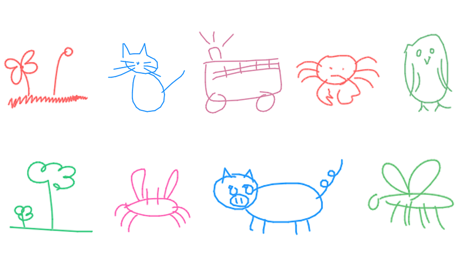
Vector drawings produced by sketch-rnn.
In our recent paper, “A Neural Representation of Sketch Drawings”, we present a generative recurrent neural network capable of producing sketches of common objects, with the goal of training a machine to draw and generalize abstract concepts in a manner similar to humans. We train our model on a dataset of hand-drawn sketches, each represented as a sequence of motor actions controlling a pen: which direction to move, when to lift the pen up, and when to stop drawing. In doing so, we created a model that potentially has many applications, from assisting the creative process of an artist, to helping teach students how to draw.

While there is a already a large body of existing work on generative modelling of images using neural networks, most of the work focuses on modelling raster images represented as a 2D grid of pixels. While these models are currently able to generate realistic images, due to the high dimensionality of a 2D grid of pixels, a key challenge for them is to generate images with coherent structure. For example, these models sometimes produce amusing images of cats with three or more eyes, or dogs with multiple heads.
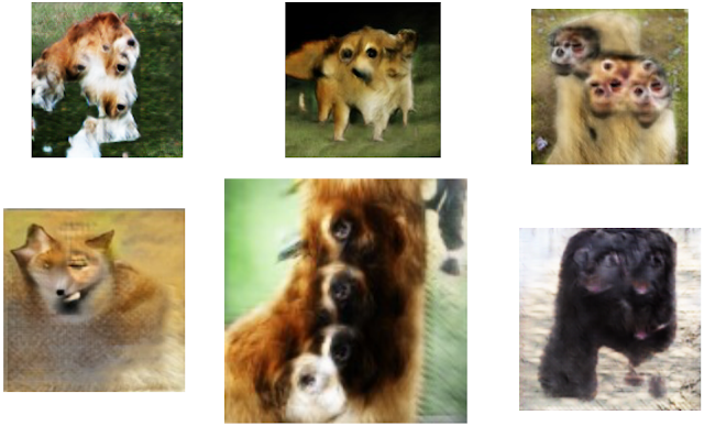
Examples of animals generated with the wrong number of body parts, produced using previous GAN models trained on 128x128 ImageNet dataset. The image above is Figure 29 of
Generative Adversarial Networks, Ian Goodfellow, NIPS 2016 Tutorial.
In this work, we investigate a lower-dimensional vector-based representation inspired by how people draw. Our model, sketch-rnn, is based on the sequence-to-sequence (seq2seq) autoencoder framework. It incorporates variational inference and utilizes hypernetworks as recurrent neural network cells. The goal of a seq2seq autoencoder is to train a network to encode an input sequence into a vector of floating point numbers, called a latent vector, and from this latent vector reconstruct an output sequence using a decoder that replicates the input sequence as closely as possible.
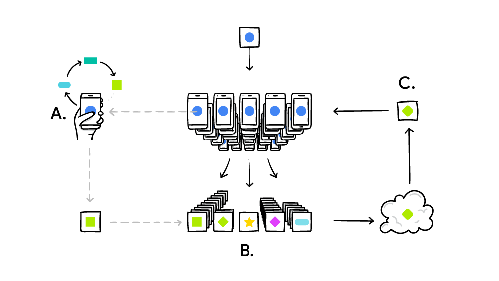
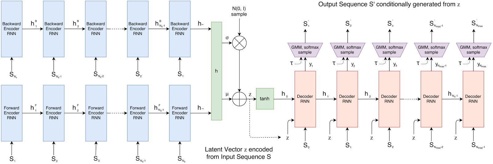
Schematic of sketch-rnn.
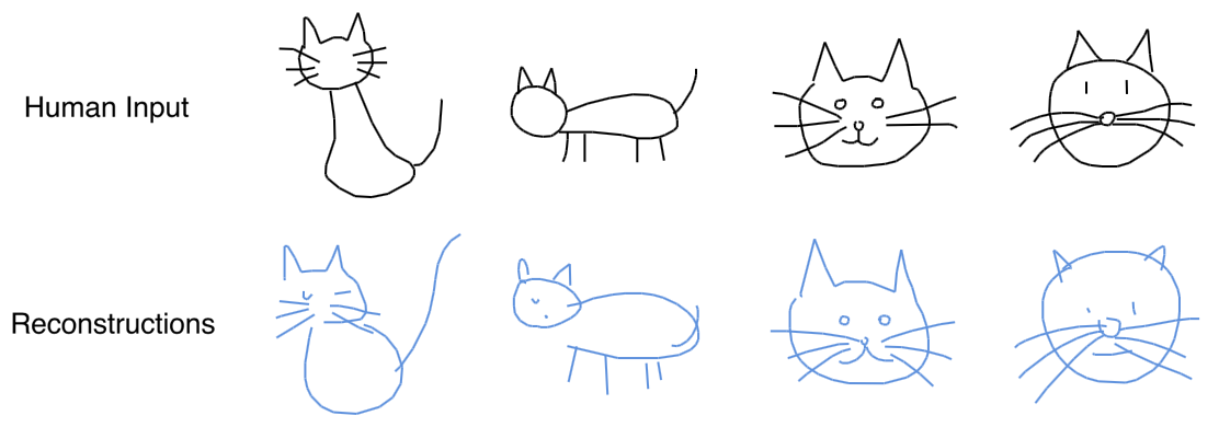
In our model, we deliberately add noise to the latent vector. In our paper, we show that by inducing noise into the communication channel between the encoder and the decoder, the model is no longer be able to reproduce the input sketch exactly, but instead must learn to capture the essence of the sketch as a noisy latent vector. Our decoder takes this latent vector and produces a sequence of motor actions used to construct a new sketch. In the figure below, we feed several actual sketches of cats into the encoder to produce reconstructed sketches using the decoder.
Reconstructions from a model trained on cat sketches.

It is important to emphasize that the reconstructed cat sketches are not copies of the input sketches, but are instead 
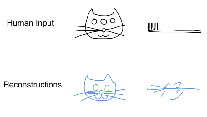
new sketches of cats with similar characteristics as the inputs. To demonstrate that the model is not simply copying from the input sequence, and that it actually learned something about the way people draw cats, we can try to feed in non-standard sketches into the encoder:
When we feed in a sketch of a three-eyed cat, the model generates a similar looking cat that has two eyes instead, suggesting that our model has learned that cats usually only have two eyes. To show that our model is not simply choosing the closest normal-looking cat from a large collection of memorized cat-sketches, we can try to input something totally different, like a sketch of a toothbrush. We see that the network generates a cat-like figure with long whiskers that mimics the features and orientation of the toothbrush. This suggests that the network has learned to encode an input sketch into a set of abstract cat-concepts embedded into the latent vector, and is also able to reconstruct an entirely new sketch based on this latent vector.

Not convinced? We repeat the experiment again on a model trained on pig sketches and arrive at similar conclusions. When presented with an eight-legged pig, the model generates a similar pig with only four legs. If we feed a truck into the pig-drawing model, we get a pig that looks a bit like the truck.
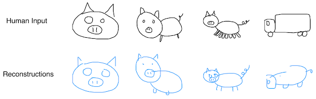
Reconstructions from a model trained on pig sketches.
To investigate how these latent vectors encode conceptual animal features, in the figure below, we first obtain two latent vectors encoded from two very different pigs, in this case a pig head (in the green box) and a full pig (in the orange box). We want to get a sense of how our model learned to represent pigs, and one way to do this is to interpolate between the two different latent vectors, and visualize each generated sketch from each interpolated latent vector. In the figure below, we visualize how the sketch of the pig head slowly morphs into the sketch of the full pig, and in the process show how the model organizes the concepts of pig sketches. We see that the latent vector controls the relatively position and size of the nose relative to the head, and also the existence of the body and legs in the sketch.
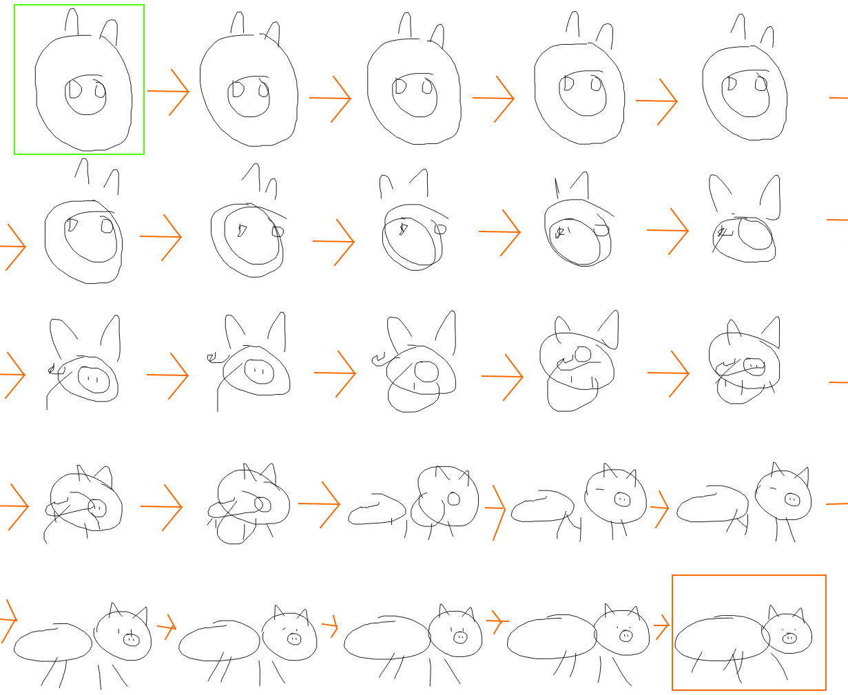
Latent space interpolations generated from a model trained on pig sketches.
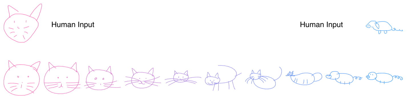
We would also like to know if our model can learn representations of multiple animals, and if so, what would they look like? In the figure below, we generate sketches from interpolating latent vectors between a cat head and a full pig. We see how the representation slowly transitions from a cat head, to a cat with a tail, to a cat with a fat body, and finally into a full pig. Like a child learning to draw animals, our model learns to construct animals by attaching a head, feet, and a tail to its body. We see that the model is also able to draw cat heads that are distinct from pig heads.
Latent Space Interpolations from a model trained on sketches of both cats and pigs.
These interpolation examples suggest that the latent vectors indeed encode conceptual features of a sketch. But can we use these features to augment other sketches without such features - for example, adding a body to a cat's head?
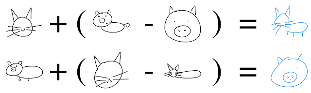
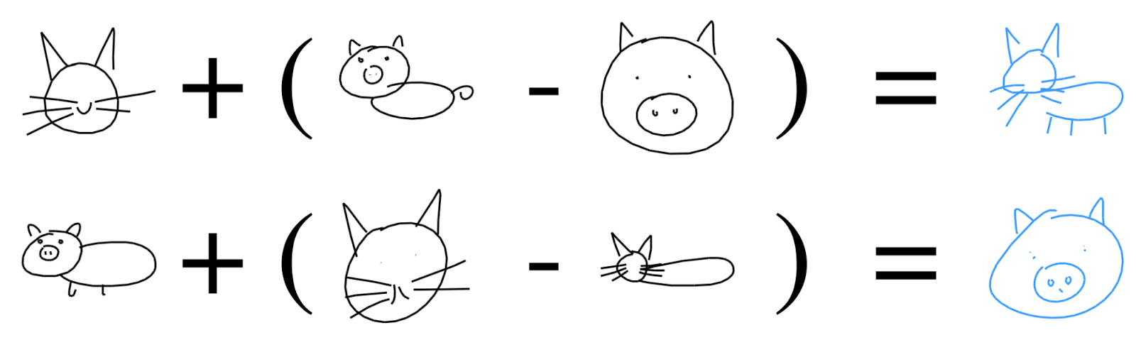
Learned relationships between abstract concepts, explored using latent vector arithmetic.
Indeed, we find that sketch drawing analogies are possible for our model trained on both cat and pig sketches. For example, we can subtract the latent vector of an encoded pig head from the latent vector of a full pig, to arrive at a vector that represents the concept of a body. Adding this difference to the latent vector of a cat head results in a full cat (i.e. cat head + body = full cat). These drawing analogies allow us to explore how the model organizes its latent space to represent different concepts in the manifold of generated sketches.

Creative Applications
In addition to the research component of this work, we are also super excited about potential creative applications of sketch-rnn. For instance, even in the simplest use case, pattern designers can apply sketch-rnn to generate a large number of similar, but unique designs for textile or wallpaper prints.
Similar, but unique cats, generated from a single input sketch (green and yellow boxes).
As we saw earlier, a model trained to draw pigs can be made to draw pig-like trucks if given an input sketch of a truck. We can extend this result to applications that might help creative designers come up with abstract designs that can resonate more with their target audience.

For instance, in the figure below, we feed sketches of four different chairs into our cat-drawing model to produce four chair-like cats. We can go further and incorporate the interpolation methodology described earlier to explore the latent space of chair-like cats, and produce a large grid of generated designs to select from.
Exploring the latent space of generated chair-cats.
Exploring the latent space between different objects can potentially enable creative designers to find interesting intersections and relationships between different drawings.
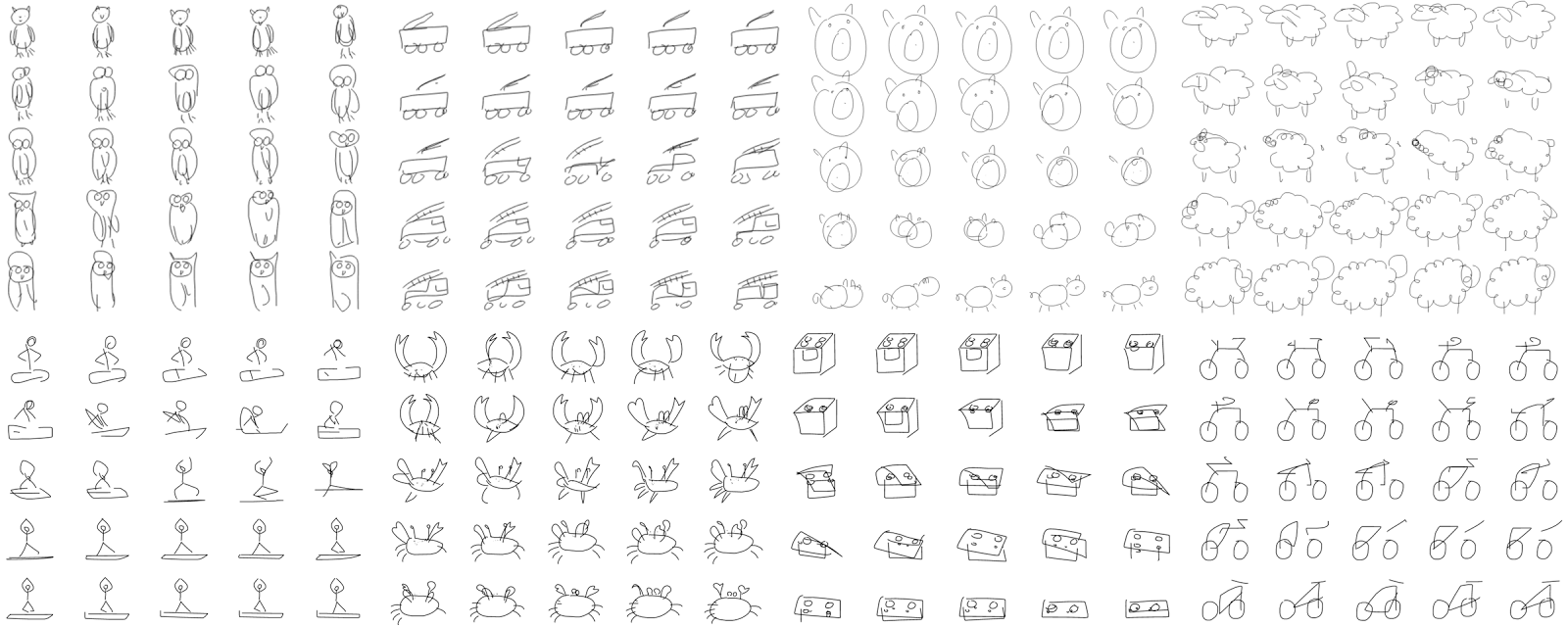
Exploring the latent space of generated sketches of everyday objects.
Latent space interpolation from left to right, and then top to bottom.
We can also use the decoder module of sketch-rnn as a standalone model and train it to predict different possible endings of incomplete sketches. This technique can lead to applications where the model assists the creative process of an artist by suggesting alternative ways to finish an incomplete sketch. In the above below, we draw different incomplete sketches (in red), and have the model come up with different possible ways to complete the drawings.
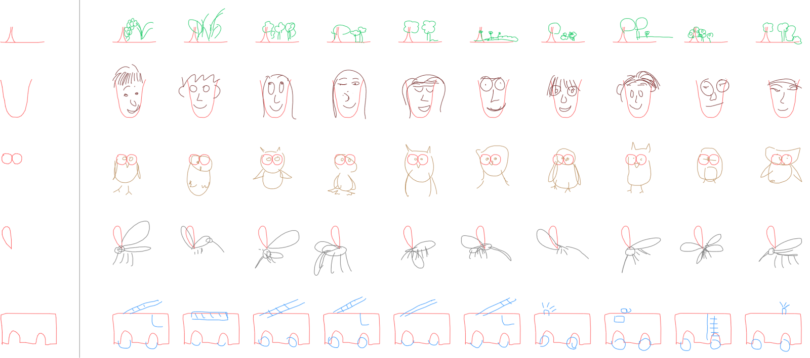
The model can start with incomplete sketches (the red partial sketches to the left of the vertical line) and automatically generate different completions.
We can take this concept even further, and have different models complete the same incomplete sketch. In the figures below, we see how to make the same circle and square figures become a part of various ants, flamingos, helicopters, owls, couches and even paint brushes. By using a diverse set of models trained to draw various objects, designers can explore creative ways to communicate meaningful visual messages to their audience.
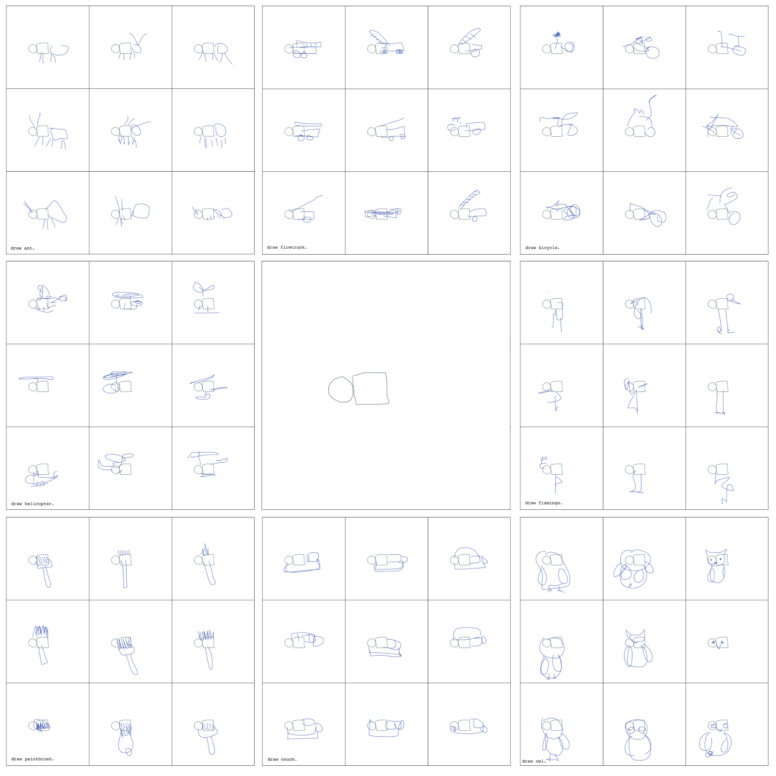
Predicting the endings of the same circle and square figures (center) using various sketch-rnn models trained to draw different objects.
We are very excited about the future possibilities of generative vector image modelling. These models will enable many exciting new creative applications in a variety of different directions. They can also serve as a tool to help us improve our understanding of our own creative thought processes. Learn more about sketch-rnn by reading our paper, “A Neural Representation of Sketch Drawings”.

Acknowledgements
We thank Ian Johnson, Jonas Jongejan, Martin Wattenberg, Mike Schuster, Ben Poole, Kyle Kastner, Junyoung Chung, Kyle McDonald for their help with this project. This work was done as part of the Google Brain Residency program.

Introducing tf-seq2seq: An Open Source Sequence-to-Sequence Framework in TensorFlow


(Crossposted on the Google Open Source Blog)

Last year, we announced Google Neural Machine Translation (GNMT), a sequence-to-sequence (“seq2seq”) model which is now used in Google Translate production systems. While GNMT achieved huge improvements in translation quality, its impact was limited by the fact that the framework for training these models was unavailable to external researchers.

Today, we are excited to introduce tf-seq2seq, an open source seq2seq framework in TensorFlow that makes it easy to experiment with seq2seq models and achieve state-of-the-art results. To that end, we made the tf-seq2seq codebase clean and modular, maintaining full test coverage and documenting all of its functionality.

Our framework supports various configurations of the standard seq2seq model, such as depth of the encoder/decoder, attention mechanism, RNN cell type, or beam size. This versatility allowed us to discover optimal hyperparameters and outperform other frameworks, as described in our paper, “Massive Exploration of Neural Machine Translation Architectures.”
A seq2seq model translating from Mandarin to English. At each time step, the encoder takes in one Chinese character and its own previous state (black arrow), and produces an output vector (blue arrow). The decoder then generates an English translation word-by-word, at each time step taking in the last word, the previous state, and a weighted combination of all the outputs of the encoder (aka attention [3], depicted in blue) and then producing the next English word. Please note that in our implementation we use wordpieces [4] to handle rare words.
In addition to machine translation, tf-seq2seq can also be applied to any other sequence-to-sequence task (i.e. learning to produce an output sequence given an input sequence), including machine summarization, image captioning, speech recognition, and conversational modeling. We carefully designed our framework to maintain this level of generality and provide tutorials, preprocessed data, and other utilities for machine translation.

We hope that you will use tf-seq2seq to accelerate (or kick off) your own deep learning research. We also welcome your contributions to our GitHub repository, where we have a variety of open issues that we would love to have your help with!

Acknowledgments:
We’d like to thank Eugene Brevdo, Melody Guan, Lukasz Kaiser, Quoc V. Le, Thang Luong, and Chris Olah for all their help. For a deeper dive into how seq2seq models work, please see the resources below.

References:
[1] Massive Exploration of Neural Machine Translation Architectures, Denny Britz, Anna Goldie, Minh-Thang Luong, Quoc Le
[2] Sequence to Sequence Learning with Neural Networks, Ilya Sutskever, Oriol Vinyals, Quoc V. Le. NIPS, 2014
[3] Neural Machine Translation by Jointly Learning to Align and Translate, Dzmitry Bahdanau, Kyunghyun Cho, Yoshua Bengio. ICLR, 2015
[4] Google’s Neural Machine Translation System: Bridging the Gap between Human and Machine Translation, Yonghui Wu, Mike Schuster, Zhifeng Chen, Quoc V. Le, Mohammad Norouzi, Wolfgang Macherey, Maxim Krikun, Yuan Cao, Qin Gao, Klaus Macherey, Jeff Klingner, Apurva Shah, Melvin Johnson, Xiaobing Liu, Łukasz Kaiser, Stephan Gouws, Yoshikiyo Kato, Taku Kudo, Hideto Kazawa, Keith Stevens, George Kurian, Nishant Patil, Wei Wang, Cliff Young, Jason Smith, Jason Riesa, Alex Rudnick, Oriol Vinyals, Greg Corrado, Macduff Hughes, Jeffrey Dean. Technical Report, 2016
[5] Attention and Augmented Recurrent Neural Networks, Chris Olah, Shan Carter. Distill, 2016
[6] Neural Machine Translation and Sequence-to-sequence Models: A Tutorial, Graham Neubig
[7] Sequence-to-Sequence Models, TensorFlow.org

Announcing the 2017 Google PhD Fellows for North America, Europe and the Middle East


Google created the PhD Fellowship program in 2009 to recognize and support outstanding graduate students doing exceptional research in Computer Science and related disciplines. Now in its eighth year, our fellowship program has supported hundreds of future faculty, industry researchers, innovators and entrepreneurs.

Reflecting our continuing commitment to supporting and building relationships with the academic community, we are excited to announce the 33 recipients from North America, Europe and the Middle East. We offer our sincere congratulations to Google’s 2017 Class of Google PhD Fellows.

Algorithms, Optimizations and Markets
Chiu Wai Sam Wong, University of California, Berkeley
Eric Balkanski, Harvard University
Haifeng Xu, University of Southern California

Human-Computer Interaction
Motahhare Eslami, University of Illinois, Urbana-Champaign
Sarah D'Angelo, Northwestern University
Sarah Mcroberts, University of Minnesota - Twin Cities

Machine Learning
Aude Genevay, Fondation Sciences Mathématiques de Paris
Dustin Tran, Columbia University
Jamie Hayes, University College London
Martin Arjovsky, New York University
Taco Cohen, University of Amsterdam
Yuhuai Wu, University of Toronto
Yunye Gong, Cornell University

Machine Perception, Speech Technology and Computer Vision
Franziska Müller, Saarland University - Saarbrücken GSCS and MPI Institute for Informatics
George Trigeorgis, Imperial College London
Iro Armeni, Stanford University
Saining Xie, University of California, San Diego
Yu-Chuan Su, University of Texas, Austin

Natural Language Processing
Jianpeng Cheng, The University of Edinburgh
Kevin Clark, Stanford University
Tim Rocktaschel, University College London

Privacy and Security
Romain Gay, ENS - École Normale Supérieure
Xi He, Duke University
Yupeng Zhang, University of Maryland, College Park

Programming Languages and Software Engineering
Christoffer Quist Adamsen, Aarhus University
Muhammad Ali Gulzar, University of California, Los Angeles
Oded Padon, Tel-Aviv University

Structured Data and Database Management
Amir Shaikhha, EPFL CS
Jingbo Shang, University of Illinois, Urbana-Champaign

Systems and Networking
Ahmed M. Said Mohamed Tawfik Issa, Georgia Institute of Technology
Khanh Nguyen, University of California, Irvine
Radhika Mittal, University of California, Berkeley
Ryan Beckett, Princeton University

Predicting Properties of Molecules with Machine Learning


Recently there have been many exciting applications of machine learning (ML) to chemistry, particularly in chemical search problems, from drug discovery and battery design to finding better OLEDs and catalysts. Historically, chemists have used numerical approximations to Schrödinger’s equation, such as Density Functional Theory (DFT), in these sorts of chemical searches. However, the computational cost of these approximations limits the size of the search. In the hope of enabling larger searches, several research groups have created ML models to predict chemical properties using training data generated by DFT (e.g. Rupp et al. and Behler and Parrinello). Expanding upon this previous work, we have been applying various modern ML methods to the QM9 benchmark –a public collection of molecules paired with DFT-computed electronic, thermodynamic, and vibrational properties.

We have recently posted two papers describing our research in this area that grew out of a collaboration between the Google Brain Team, Google Accelerated Science, DeepMind, and the University of Basel. The first paper includes a new featurization of molecules and a systematic assessment of a multitude of machine learning methods on the QM9 benchmark. After trying many existing approaches on this benchmark, we worked on improving the most promising deep neural network models.

The resulting second paper, “Neural Message Passing for Quantum Chemistry,” describes a model family called Message Passing Neural Networks (MPNNs), which are defined abstractly enough to include many previous neural net models that are invariant to graph symmetries. We developed novel variations within the MPNN family which significantly outperform all baseline methods on the QM9 benchmark, with improvements of nearly a factor of four on some targets.

One reason molecular data is so interesting from a machine learning standpoint is that one natural representation of a molecule is as a graph with atoms as nodes and bonds as edges. Models that can leverage inherent symmetries in data will tend to generalize better — part of the success of convolutional neural networks on images is due to their ability to incorporate our prior knowledge about the invariances of image data (e.g. a picture of a dog shifted to the left is still a picture of a dog). Invariance to graph symmetries is a particularly desirable property for machine learning models that operate on graph data, and there has been a lot of interesting research in this area as well (e.g. Li et al., Duvenaud et al., Kearnes et al., Defferrard et al.). However, despite this progress, much work remains. We would like to find the best versions of these models for chemistry (and other) applications and map out the connections between different models proposed in the literature.

Our MPNNs set a new state of the art for predicting all 13 chemical properties in QM9. On this particular set of molecules, our model can predict 11 of these properties accurately enough to potentially be useful to chemists, but up to 300,000 times faster than it would take to simulate them using DFT. However, much work remains to be done before MPNNs can be of real practical use to chemists. In particular, MPNNs must be applied to a significantly more diverse set of molecules (e.g. larger or with a more varied set of heavy atoms) than exist in QM9. Of course, even with a realistic training set, generalization to very different molecules could still be poor. Overcoming both of these challenges will involve making progress on questions–such as generalization–that are at the heart of machine learning research.

Predicting the properties of molecules is a practically important problem that both benefits from advanced machine learning techniques and presents interesting fundamental research challenges for learning algorithms. Eventually, such predictions could aid the design of new medicines and materials that benefit humanity. At Google, we feel that it’s important to disseminate our research and to help train new researchers in machine learning. As such, we are delighted that the first and second authors of our MPNN paper are Google Brain residents.

Federated Learning: Collaborative Machine Learning without Centralized Training Data


Standard machine learning approaches require centralizing the training data on one machine or in a datacenter. And Google has built one of the most secure and robust cloud infrastructures for processing this data to make our services better. Now for models trained from user interaction with mobile devices, we're introducing an additional approach: Federated Learning.

Federated Learning enables mobile phones to collaboratively learn a shared prediction model while keeping all the training data on device, decoupling the ability to do machine learning from the need to store the data in the cloud. This goes beyond the use of local models that make predictions on mobile devices (like the Mobile Vision API and On-Device Smart Reply) by bringing model training to the device as well.

It works like this: your device downloads the current model, improves it by learning from data on your phone, and then summarizes the changes as a small focused update. Only this update to the model is sent to the cloud, using encrypted communication, where it is immediately averaged with other user updates to improve the shared model. All the training data remains on your device, and no individual updates are stored in the cloud.
Your phone personalizes the model locally, based on your usage (A). Many users' updates are aggregated (B) to form a consensus change (C) to the shared model, after which the procedure is repeated.
Federated Learning allows for smarter models, lower latency, and less power consumption, all while ensuring privacy. And this approach has another immediate benefit: in addition to providing an update to the shared model, the improved model on your phone can also be used immediately, powering experiences personalized by the way you use your phone.

We're currently testing Federated Learning in Gboard on Android, the Google Keyboard. When Gboard shows a suggested query, your phone locally stores information about the current context and whether you clicked the suggestion. Federated Learning processes that history on-device to suggest improvements to the next iteration of Gboard’s query suggestion model.
To make Federated Learning possible, we had to overcome many algorithmic and technical challenges. In a typical machine learning system, an optimization algorithm like Stochastic Gradient Descent (SGD) runs on a large dataset partitioned homogeneously across servers in the cloud. Such highly iterative algorithms require low-latency, high-throughput connections to the training data. But in the Federated Learning setting, the data is distributed across millions of devices in a highly uneven fashion. In addition, these devices have significantly higher-latency, lower-throughput connections and are only intermittently available for training.

These bandwidth and latency limitations motivate our Federated Averaging algorithm, which can train deep networks using 10-100x less communication compared to a naively federated version of SGD. The key idea is to use the powerful processors in modern mobile devices to compute higher quality updates than simple gradient steps. Since it takes fewer iterations of high-quality updates to produce a good model, training can use much less communication. As upload speeds are typically much slower than download speeds, we also developed a novel way to reduce upload communication costs up to another 100x by compressing updates using random rotations and quantization. While these approaches are focused on training deep networks, we've also designed algorithms for high-dimensional sparse convex models which excel on problems like click-through-rate prediction.

Deploying this technology to millions of heterogenous phones running Gboard requires a sophisticated technology stack. On device training uses a miniature version of TensorFlow. Careful scheduling ensures training happens only when the device is idle, plugged in, and on a free wireless connection, so there is no impact on the phone's performance.
Your phone participates in Federated Learning only
when it won't negatively impact your experience.
The system then needs to communicate and aggregate the model updates in a secure, efficient, scalable, and fault-tolerant way. It's only the combination of research with this infrastructure that makes the benefits of Federated Learning possible.

Federated learning works without the need to store user data in the cloud, but we're not stopping there. We've developed a Secure Aggregation protocol that uses cryptographic techniques so a coordinating server can only decrypt the average update if 100s or 1000s of users have participated — no individual phone's update can be inspected before averaging. It's the first protocol of its kind that is practical for deep-network-sized problems and real-world connectivity constraints. We designed Federated Averaging so the coordinating server only needs the average update, which allows Secure Aggregation to be used; however the protocol is general and can be applied to other problems as well. We're working hard on a production implementation of this protocol and expect to deploy it for Federated Learning applications in the near future.

Our work has only scratched the surface of what is possible. Federated Learning can't solve all machine learning problems (for example, learning to recognize different dog breeds by training on carefully labeled examples), and for many other models the necessary training data is already stored in the cloud (like training spam filters for Gmail). So Google will continue to advance the state-of-the-art for cloud-based ML, but we are also committed to ongoing research to expand the range of problems we can solve with Federated Learning. Beyond Gboard query suggestions, for example, we hope to improve the language models that power your keyboard based on what you actually type on your phone (which can have a style all its own) and photo rankings based on what kinds of photos people look at, share, or delete.

Applying Federated Learning requires machine learning practitioners to adopt new tools and a new way of thinking: model development, training, and evaluation with no direct access to or labeling of raw data, with communication cost as a limiting factor. We believe the user benefits of Federated Learning make tackling the technical challenges worthwhile, and are publishing our work with hopes of a widespread conversation within the machine learning community.

Acknowledgements
This post reflects the work of many people in Google Research, including Blaise Agüera y Arcas, Galen Andrew, Dave Bacon, Keith Bonawitz, Chris Brumme, Arlie Davis, Jac de Haan, Hubert Eichner, Wolfgang Grieskamp, Wei Huang, Vladimir Ivanov, Chloé Kiddon, Jakub Konečný, Nicholas Kong, Ben Kreuter, Alison Lentz, Stefano Mazzocchi, Sarvar Patel, Martin Pelikan, Aaron Segal, Karn Seth, Ananda Theertha Suresh, Iulia Turc, Felix Yu, and our partners in the Gboard team.

Keeping fake listings off Google Maps


(Crossposted on the Google Security blog)

Google My Business enables millions of business owners to create listings and share information about their business on Google Maps and Search, making sure everything is up-to-date and accurate for their customers. Unfortunately, some actors attempt to abuse this service to register fake listings in order to defraud legitimate business owners, or to charge exorbitant service fees for services.

Over a year ago, we teamed up with the University of California, San Diego to research the actors behind fake listings, in order to improve our products and keep our users safe. The full report, “Pinning Down Abuse on Google Maps”, will be presented tomorrow at the 2017 International World Wide Web Conference.

Our study shows that fewer than 0.5% of local searches lead to fake listings. We’ve also improved how we verify new businesses, which has reduced the number of fake listings by 70% from its all-time peak back in June 2015.

What is a fake listing?
For over a year, we tracked the bad actors behind fake listings. Unlike email-based scams selling knock-off products online, local listing scams require physical proximity to potential victims. This fundamentally changes both the scale and types of abuse possible.

Bad actors posing as locksmiths, plumbers, electricians, and other contractors were the most common source of abuse—roughly 2 out of 5 fake listings. The actors operating these fake listings would cycle through non-existent postal addresses and disposable VoIP phone numbers even as their listings were discovered and disabled. The purported addresses for these businesses were irrelevant as the contractors would travel directly to potential victims.

Another 1 in 10 fake listings belonged to real businesses that bad actors had improperly claimed ownership over, such as hotels and restaurants. While making a reservation or ordering a meal was indistinguishable from the real thing, behind the scenes, the bad actors would deceive the actual business into paying referral fees for organic interest.

How does Google My Business verify information?
Google My Business currently verifies the information provided by business owners before making it available to users. For freshly created listings, we physically mail a postcard to the new listings’ address to ensure the location really exists. For businesses changing owners, we make an automated call to the listing’s phone number to verify the change.
Unfortunately, our research showed that these processes can be abused to get fake listings on Google Maps. Fake contractors would request hundreds of postcard verifications to non-existent suites at a single address, such as 123 Main St #456 and 123 Main St #789, or to stores that provided PO boxes. Alternatively, a phishing attack could maliciously repurpose freshly verified business listings by tricking the legitimate owner into sharing verification information sent either by phone or postcard.

Keeping deceptive businesses out — by the numbers
Leveraging our study’s findings, we’ve made significant changes to how we verify addresses and are even piloting an advanced verification process for locksmiths and plumbers. Improvements we’ve made include prohibiting bulk registrations at most addresses, preventing businesses from relocating impossibly far from their original address without additional verification, and detecting and ignoring intentionally mangled text in address fields designed to confuse our algorithms. We have also adapted our anti-spam machine learning systems to detect data discrepancies common to fake or deceptive listings.

Combined, here’s how these defenses stack up:

  • We detect and disable 85% of fake listings before they even appear on Google Maps.
  • We’ve reduced the number of abusive listings by 70% from its peak back in June 2015.
  • We’ve also reduced the number of impressions to abusive listings by 70%.

As we’ve shown, verifying local information comes with a number of unique anti-abuse challenges. While fake listings may slip through our defenses from time to time, we are constantly improving our systems to better serve both users and business owners.

And the award goes to…


Today, Google's Andrei Broder, Ravi Kumar, Prabhakar Raghavan, Sridhar Rajagopalan, and Andrew Tomkins, along with their coauthors, Farzin Maghoul, Raymie Stata, and Janet Wiener, have received the prestigious 2017 Seoul Test of Time Award for their classic paper “Graph Structure in the Web”. This award is given to the authors of a previous World Wide Web conference paper that has demonstrated significant scientific, technical, or social impact over the years. The first award, introduced in 2015, was given to Google founders Larry Page and Sergey Brin.

Originally presented in 2000 at the 9th WWW conference in Amsterdam, “Graph Structure in the Web” represents the seminal study of the structure of the World Wide Web. At the time of publication, it received the Best Paper Award from the WWW conference, and in the following 17 years proved to be highly influential, accumulating over 3,500 citations.

The paper made two major contributions to the study of the structure of the Internet. First, it reported the results of a very large scale experiment to confirm that the indegree of Web nodes is distributed according to a power law. To wit, the probability that a node of the Web graph has i incoming links is roughly proportional to 1/i2.1. Second, in contrast to previous research that assumed the Web to be almost fully connected, “Graph Structure in the Web” described a much more elaborate structure of the Web, which since then has been depicted with the iconic “bowtie” shape:
Original “bowtie” schematic from “Graph Structure in the Web”
The authors presented a refined model of the Web graph, and described several characteristic classes of Web pages:
  • the strongly connected core component, where each page is reachable from any other page,
  • the so-called IN and OUT clusters, which only have unidirectional paths to or from the core,
  • tendrils dangling from the two clusters, and tubes connecting the clusters while bypassing the core, and finally
  • disconnected components, which are isolated from the rest of the graph.
Whereas the core component is fully connected and each node can be reached from any other node, Broder et al. discovered that as a whole the Web is much more loosely connected than previously believed, while the probability that any two given pages can be reached from one another is just under 1/4.
Ravi Kumar, presenting the original paper in Amsterdam at WWW 2000
Curiously, the original study was done back in 1999 on two Altavista crawls having 200 million pages and 1.5 billion links. Today, Google indexes over 100 billion links merely within apps, and overall processes over 130 trillion web addresses in its web crawls.

Over the years, the power law was found to be characteristic of many other Web-related phenomena, including the structure of social networks and the distribution of search query frequencies. The description of the macroscopic structure of the Web graph proposed by Broder et al. provided a solid mathematical foundation for numerous subsequent studies on crawling and searching the Web, which profoundly influenced the architecture of modern search engines.

Hearty congratulations to all the authors on the well-deserved award!

Consistent Hashing with Bounded Loads


Running a large-scale web service, such as content hosting, necessarily requires load balancing — distributing clients uniformly across multiple servers such that none get overloaded. Further, it is desirable to find an allocation that does not change very much over time in a dynamic environment in which both clients and servers can be added or removed at any time. In other words, we need the allocation of clients to servers to be consistent over time.

In collaboration with Mikkel Thorup, a visiting researcher from university of Copenhagen, we developed a new efficient allocation algorithm for this problem with tight guarantees on the maximum load of each server, and studied it theoretically and empirically. We then worked with our Cloud team to implement it in Google Cloud Pub/Sub, a scalable event streaming service, and observed substantial improvement on uniformity of the load allocation (in terms of the maximum load assigned to servers) while maintaining consistency and stability objectives. In August 2016 we described our algorithm in the paper “Consistent Hashing with Bounded Loads”, and shared it on ArXiv for potential use by the broader research community.

Three months later, Andrew Rodland from Vimeo informed us that he had found the paper, implemented it in haproxy (a widely-used piece of open source software), and used it for their load balancing project at Vimeo. The results were dramatic: applying these algorithmic ideas helped them decrease the cache bandwidth by a factor of almost 8, eliminating a scaling bottleneck. He recently summarized this story in a blog post detailing his use case. Needless to say, we were excited to learn that our theoretical research was not only put into application, but also that it was useful and open-sourced.

Background
While the concept of consistent hashing has been developed in the past to deal with load balancing in dynamic environments, a fundamental issue with all the previously developed schemes is that, in certain scenarios, they may result in sub-optimal load balancing on many servers.

Additionally, both clients and servers may be added or removed periodically, and with such changes, we do not want to move too many clients. Thus, while the dynamic allocation algorithm has to always ensure a proper load balancing, it should also aim to minimize the number of clients moved after each change to the system. Such allocation problems become even more challenging when we face hard constraints on the capacity of each server - that is, each server has a capacity that the load may not exceed. Typically, we want capacities close to the average loads.

In other words, we want to simultaneously achieve both uniformity and consistency in the resulting allocations. There is a vast amount of literature on solutions in the much simpler case where the set of servers is fixed and only the client set is updated, but in this post we discuss solutions that are relevant in the fully dynamic case where both clients and servers can be added and removed.

The Algorithm
We can think about the servers as bins and clients as balls to have a similar notation with well-studied balls-to-bins stochastic processes. The uniformity objective encourages all bins to have a load roughly equal to the average density (the number of balls divided by the number of bins). For some parameter ε, we set the capacity of each bin to either floor or ceiling of the average load times (1+ε). This extra capacity allows us to design an allocation algorithm that meets the consistency objective in addition to the uniformity property.

Imagine a given range of numbers overlaid on a circle. We apply a hash function to balls and a separate hash function to bins to obtain numbers in that range that correspond to positions on that circle. We then start allocating balls in a specific order independent of their hash values (let’s say based on their ID). Then each ball is moved clockwise and is assigned to the first bin with spare capacity.
Consider the example above where 6 balls and 3 bins are assigned using two separate hash functions to random locations on the circle. For the sake of this instance, assume the capacity of each bin is set to 2. We start allocating balls in the increasing order of their ID values. Ball number 1 moves clockwise, and goes to bin C. Ball number 2 goes to A. Balls 3 and 4 go to bin B. Ball number 5 goes to bin C. Then ball number 6 moves clockwise and hits bin B first. However bin B has capacity 2 and already contains balls 3 and 4. So ball 6 keeps moving to reach bin C but that bin is also full. Finally, ball 6 ends up in bin A that has a spare slot for it.

Upon any update in the system (ball or bin insertion/deletion), the allocation is recomputed to keep the uniformity objective. The art of the analysis is to show that a small update (a few number of insertions and deletions) results in minor changes in the state of the allocation and therefore the consistency objective is met. In our paper we show that every ball removal or insertion in the system results in O(1/ε2) movements of other balls. The most important thing about this upper bound is that it is independent of the total number of balls or bins in the system. So if the number of balls or bins are doubled, this bound will not change. Having an upper bound independent of the number of balls or bins introduces room for scalability as the consistency objective is not violated if we move to bigger instances. Simulations for the number of movements (relocations) per update is shown below when an update occurs on a bin/server.
The red curve shows the average number of movements and the blue bars indicate the variance for different values of ε (the x-axis). The dashed curve is the upper bound suggested by our theoretical results which fits nicely as a prediction of the actual number of movements. Furthermore, for any value of ε, we know the load of each bin is at most (1+ε) times the average load. Below we see the load distribution of bins for different values of ε=0.1, ε=0.3 and ε=0.9.
The distribution of loads for several values of ε. The load distribution is nearly uniform covering all ranges of loads from 0 to (1+ε) times average, and many bins with load equal to (1+ε) times average.
As one can see there is a tradeoff — a lower ε helps with uniformity but not with consistency, while larger ε values help with consistency. A lower ε will ensure that many loads will be equal to the hard capacity limit of (1+ε) times the average, and the rest have a decaying distribution.

When providing content hosting services, one must be ready to face a variety of instances with different characteristics. This consistent hashing scheme is ideal for such scenarios as it performs well even for worst-case instances.

While our internal results are exciting, we are even more pleased that the broader community found our solution useful enough to open-source, allowing anyone to use this algorithm. If you are interested in further details of this research, please see the paper on ArXiv, and stay tuned for more research from the NYC Algorithms Team!

Acknowledgements:
We would like to thank Alex Totok, Matt Gruskin, Sergey Kondratyev and Haakon Ringberg from the Google Cloud Pub/Sub team, and of course Mikkel Thorup for his invaluable contributions to this paper.

Announcing AudioSet: A Dataset for Audio Event Research


Systems able to recognize sounds familiar to human listeners have a wide range of applications, from adding sound effect information to automatic video captions, to potentially allowing you to search videos for specific audio events. Building Deep Learning systems to do this relies heavily on both a large quantity of computing (often from highly parallel GPUs), and also – and perhaps more importantly – on significant amounts of accurately-labeled training data. However, research in environmental sound recognition is limited by currently available public datasets.

In order to address this, we recently released AudioSet, a collection of over 2 million ten-second YouTube excerpts labeled with a vocabulary of 527 sound event categories, with at least 100 examples for each category. Announced in our paper at the IEEE International Conference on Acoustics, Speech, and Signal Processing, AudioSet provides a common, realistic-scale evaluation task for audio event detection and a starting point for a comprehensive vocabulary of sound events, designed to advance research into audio event detection and recognition.
Developing an Ontology
When we started on this work last year, our first task was to define a vocabulary of sound classes that provided a consistent level of detail over the spectrum of sound events we planned to label. Defining this ontology was necessary to avoid problems of ambiguity and synonyms; without this, we might end up trying to differentiate “Timpani” from “Kettle drum”, or “Water tap” from “Faucet”. Although a number of scientists have looked at how humans organize sound events, the few existing ontologies proposed have been small and partial. To build our own, we searched the web for phrases like “Sounds, such as X and Y”, or “X, Y, and other sounds”. This gave us a list of sound-related words which we manually sorted into a hierarchy of over 600 sound event classes ranging from “Child speech” to “Ukulele” to “Boing”. To make our taxonomy as comprehensive as possible, we then looked at comparable lists of sound events (for instance, the Urban Sound Taxonomy) to add significant classes we may have missed and to merge classes that weren't well defined or well distinguished. You can explore our ontology here.
The top two levels of the AudioSet ontology.
From Ontology to Labeled Data
With our new ontology in hand, we were able to begin collecting human judgments of where the sound events occur. This, too, raises subtle problems: unlike the billions of well-composed photographs available online, people don’t typically produce “well-framed” sound recordings, much less provide them with captions. We decided to use 10 second sound snippets as our unit; anything shorter becomes very difficult to identify in isolation. We collected candidate snippets for each of our classes by taking random excerpts from YouTube videos whose metadata indicated they might contain the sound in question (“Dogs Barking for 10 Hours”). Each snippet was presented to a human labeler with a small set of category names to be confirmed (“Do you hear a Bark?”). Subsequently, we proposed snippets whose content was similar to examples that had already been manually verified to contain the class, thereby finding examples that were not discoverable from the metadata. Because some classes were much harder to find than others – particularly the onomatopoeia words like “Squish” and “Clink” – we adapted our segment proposal process to increase the sampling for those categories. For more details, see our paper on the matching technique.

AudioSet provides the URLs of each video excerpt along with the sound classes that the raters confirmed as present, as well as precalculated audio features from the same classifier used to generate audio features for the updated YouTube 8M Dataset. Below is a histogram of the number of examples per class:
The total number of videos for selected classes in AudioSet.
You can browse this data at the AudioSet website which lets you view all the 2 million excerpts for all the classes.
A few of the segments representing the class “Violin, fiddle”.
Quality Assessment
Once we had a substantial set of human ratings, we conducted an internal Quality Assessment task where, for most of the classes, we checked 10 examples of excerpts that the annotators had labeled with that class. This revealed a significant number of classes with inaccurate labeling: some, like “Dribble” (uneven water flow) and “Roll” (a hard object moving by rotating) had been systematically confused (as basketball dribbling and drum rolls, respectively); some such as “Patter” (footsteps of small animals) and “Sidetone” (background sound on a telephony channel) were too difficult to label and/or find examples for, even with our content-based matching. We also looked at the behavior of a classifier trained on the entire dataset and found a number of frequent confusions indicating separate classes that were not really distinct, such as “Jingle” and “Tinkle”.

To address these “problem” classes, we developed a re-rating process by labeling groups of classes that span (and thus highlight) common confusions, and created instructions for the labeler to be used with these sounds. This re-rating has led to multiple improvements – merged classes, expanded coverage, better descriptions – that we were able to incorporate in this release. This iterative process of labeling and assessment has been particularly effective in shaking out weaknesses in the ontology.

A Community Dataset
By releasing AudioSet, we hope to provide a common, realistic-scale evaluation task for audio event detection, as well as a starting point for a comprehensive vocabulary of sound events. We would like to see a vibrant sound event research community develop, including through external efforts such as the DCASE challenge series. We will continue to improve the size, coverage, and accuracy of this data and plan to make a second release in the coming months when our rerating process is complete. We additionally encourage the research community to continue to refine our ontology, which we have open sourced on GitHub. We believe that with this common focus, sound event recognition will continue to advance and will allow machines to understand sounds similar to the way we do, enabling new and exciting applications.

Acknowledgments:
AudioSet is the work of Jort F. Gemmeke, Dan Ellis, Dylan Freedman, Shawn Hershey, Aren Jansen, Wade Lawrence, Channing Moore, Manoj Plakal, and Marvin Ritter, with contributions from Sami Abu-El-Hajia, Sourish Chaudhuri, Victor Gomes, Nisarg Kothari, Dick Lyon, Sobhan Naderi Parizi, Paul Natsev, Brian Patton, Rif A. Saurous, Malcolm Slaney, Ron Weiss, and Kevin Wilson.

Adding Sound Effect Information to YouTube Captions


The effect of audio on our perception of the world can hardly be overstated. Its importance as a communication medium via speech is obviously the most familiar, but there is also significant information conveyed by ambient sounds. These ambient sounds create context that we instinctively respond to, like getting startled by sudden commotion, the use of music as a narrative element, or how laughter is used as an audience cue in sitcoms.

Since 2009, YouTube has provided automatic caption tracks for videos, focusing heavily on speech transcription in order to make the content hosted more accessible. However, without similar descriptions of the ambient sounds in videos, much of the information and impact of a video is not captured by speech transcription alone. To address this, we announced the addition of sound effect information to the automatic caption track in YouTube videos, enabling greater access to the richness of all the audio content.

In this post, we discuss the backend system developed for this effort, a collaboration among the Accessibility, Sound Understanding and YouTube teams that used machine learning (ML) to enable the first ever automatic sound effect captioning system for YouTube.
Click the CC button to see the sound effect captioning system in action.
The application of ML – in this case, a Deep Neural Network (DNN) model – to the captioning task presented unique challenges. While the process of analyzing the time-domain audio signal of a video to detect various ambient sounds is similar to other well known classification problems (such as object detection in images), in a product setting the solution faces additional difficulties. In particular, given an arbitrary segment of audio, we need our models to be able to 1) detect the desired sounds, 2) temporally localize the sound in the segment and 3) effectively integrate it in the caption track, which may have parallel and independent speech recognition results.

A DNN Model for Ambient Sound
The first challenge we faced in developing the model was the task of obtaining enough labeled data suitable for training our neural network. While labeled ambient sound information is difficult to come by, we were able to generate a large enough dataset for training using weakly labeled data. But of all the ambient sounds in a given video, which ones should we train our DNN to detect?

For the initial launch of this feature, we chose [APPLAUSE], [MUSIC] and [LAUGHTER], prioritized based upon our analysis of human-created caption tracks that indicates that they are among the most frequent sounds that are manually captioned. While the sound space is obviously far richer and provides even more contextually relevant information than these three classes, the semantic information conveyed by these sound effects in the caption track is relatively unambiguous, as opposed to sounds like [RING] which raises the question of “what was it that rang – a bell, an alarm, a phone?”

Much of our initial work on detecting these ambient sounds also included developing the infrastructure and analysis frameworks to enable scaling for future work, including both the detection of sound events and their integration into the automatic caption track. Investing in the development of this infrastructure has the added benefit of allowing us to easily incorporate more sound types in the future, as we expand our algorithms to understand a wider vocabulary of sounds (e.g. [RING], [KNOCK], [BARK]). In doing so, we will be able to incorporate the detected sounds into the narrative to provide more relevant information (e.g. [PIANO MUSIC], [RAUCOUS APPLAUSE]) to viewers.

Dense Detections to Captions
When a video is uploaded to YouTube, the sound effect recognition pipeline runs on the audio stream in the video. The DNN looks at short segments of audio and predicts whether that segment contains any one of the sound events of interest – since multiple sound effects can co-occur, our model makes a prediction at each time step for each of the sound effects. The segment window is then slid to the right (i.e. a slightly later point in time) and the model is used to make a prediction again, and so on till it reaches the end. This results in a dense stream the (likelihood of) presence of each of the sound events in our vocabulary at 100 frames per second.

The dense prediction stream is not directly exposed to the user, of course, since that would result in captions flickering on and off, and because we know that a number of sound effects have some degree of temporal continuity when they occur; e.g. “music” and “applause” will usually be present for a few seconds at least. To incorporate this intuition, we smooth over the dense prediction stream using a modified Viterbi algorithm containing two states: ON and OFF, with the predicted segments for each sound effect corresponding to the ON state. The figure below provides an illustration of the process in going from the dense detections to the final segments determined to contain sound effects of interest.
(Left) The dense sequence of probabilities from our DNN for the occurrence over time of single sound category in a video. (Center) Binarized segments based on the modified Viterbi algorithm. (Right) The duration-based filter removes segments that are shorter in duration than desired for the class.
A classification-based system such as this one will certainly have some errors, and needs to be able to trade off false positives against missed detections as per the product goals. For example, due to the weak labels in the training dataset, the model was often confused between events that tended to co-occur. For example, a segment labeled “laugh” would usually contain both speech and laughter and the model for “laugh” would have a hard time distinguishing them in test data. In our system, we allow further restrictions based on time spent in the ON state (i.e. do not determine sound X to be detected unless it was determined to be present for at least Y seconds) to push performance toward a desired point in the precision-recall curve.

Once we were satisfied with the performance of our system in temporally localizing sound effect captions based on our offline evaluation metrics, we were faced with the following: how do we combine the sound effect and speech captions to create a single automatic caption track, and how (or when) do we present sound effect information to the user to make it most useful to them?

Adding Sound Effect Information into the Automatic Captions Track
Once we had a system capable of accurately detecting and classifying the ambient sounds in video, we investigated how to convey that information to the viewer in an effective way. In collaboration with our User Experience (UX) research teams, we explored various design options and tested them in a qualitative pilot usability study. The participants of the study had different hearing levels and varying needs for captions. We asked participants a number of questions including whether it improved their overall experience, their ability to follow events in the video and extract relevant information from the caption track, to understand the effect of variables such as:
  • Using separate parts of the screen for speech and sound effect captions.
  • Interleaving the speech and sound effect captions as they occur.
  • Only showing sound effect captions at the end of sentences or when there is a pause in speech (even if they occurred in the middle of speech).
  • How hearing users perceive captions when watching with the sound off.
While it wasn’t surprising that almost all users appreciated the added sound effect information when it was accurate, we also paid specific attention to the feedback when the sound detection system made an error (a false positive when determining presence of a sound, or failing to detect an occurrence). This presented a surprising result: when sound effect information was incorrect, it did not detract from the participant’s experience in roughly 50% of the cases. Based upon participant feedback, the reasons for this appear to be:
  • Participants who could hear the audio were able to ignore the inaccuracies.
  • Participants who could not hear the audio interpreted the error as the presence of a sound event, and that they had not missed out on critical speech information.
Overall, users reported that they would be fine with the system making the occasional mistake as long as it was able to provide good information far more often than not.

Looking Forward
Our work toward enabling automatic sound effect captions for YouTube videos and the initial rollout is a step toward making the richness of content in videos more accessible to our users who experience videos in different ways and in different environments that require captions. We’ve developed a framework to enrich the automatic caption track with sound effects, but there is still much to be done here. We hope that this will spur further work and discussion in the community around improving captions using not only automatic techniques, but also around ways to make creator-generated and community-contributed caption tracks richer (including perhaps, starting with the auto-captions) and better to further improve the viewing experience for our users.