Author Archives: Research Blog

Portrait mode on the Pixel 2 and Pixel 2 XL smartphones


Portrait mode, a major feature of the new Pixel 2 and Pixel 2 XL smartphones, allows anyone to take professional-looking shallow depth-of-field images. This feature helped both devices earn DxO's highest mobile camera ranking, and works with both the rear-facing and front-facing cameras, even though neither is dual-camera (normally required to obtain this effect). Today we discuss the machine learning and computational photography techniques behind this feature.
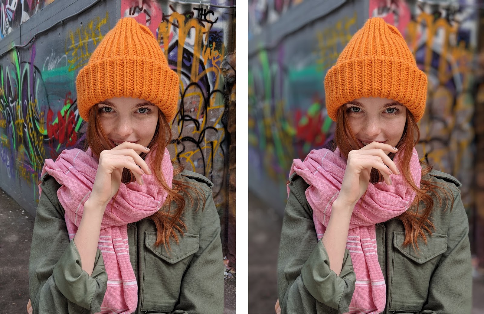
HDR+ picture without (left) and with (right) portrait mode. Note how portrait mode’s synthetic shallow depth of field helps suppress the cluttered background and focus attention on the main subject. Click on these links in the caption to see full resolution versions. Photo by Matt Jones
What is a shallow depth-of-field image?
A single-lens reflex (SLR) camera with a big lens has a shallow depth of field, meaning that objects at one distance from the camera are sharp, while objects in front of or behind that "in-focus plane" are blurry. Shallow depth of field is a good way to draw the viewer's attention to a subject, or to suppress a cluttered background. Shallow depth of field is what gives portraits captured using SLRs their characteristic artistic look.

The amount of blur in a shallow depth-of-field image depends on depth; the farther objects are from the in-focus plane, the blurrier they appear. The amount of blur also depends on the size of the lens opening. A 50mm lens with an f/2.0 aperture has an opening 50mm/2 = 25mm in diameter. With such a lens, objects that are even a few inches away from the in-focus plane will appear soft.

One other parameter worth knowing about depth of field is the shape taken on by blurred points of light. This shape is called bokeh, and it depends on the physical structure of the lens's aperture. Is the bokeh circular? Or is it a hexagon, due to the six metal leaves that form the aperture inside some lenses? Photographers debate tirelessly about what constitutes good or bad bokeh.

Synthetic shallow depth of field images
Unlike SLR cameras, mobile phone cameras have a small, fixed-size aperture, which produces pictures with everything more or less in focus. But if we knew the distance from the camera to points in the scene, we could replace each pixel in the picture with a blur. This blur would be an average of the pixel's color with its neighbors, where the amount of blur depends on distance of that scene point from the in-focus plane. We could also control the shape of this blur, meaning the bokeh.

How can a cell phone estimate the distance to every point in the scene? The most common method is to place two cameras close to one another – so-called dual-camera phones. Then, for each patch in the left camera's image, we look for a matching patch in the right camera's image. The position in the two images where this match is found gives the depth of that scene feature through a process of triangulation. This search for matching features is called a stereo algorithm, and it works pretty much the same way our two eyes do.

A simpler version of this idea, used by some single-camera smartphone apps, involves separating the image into two layers – pixels that are part of the foreground (typically a person) and pixels that are part of the background. This separation, sometimes called semantic segmentation, lets you blur the background, but it has no notion of depth, so it can't tell you how much to blur it. Also, if there is an object in front of the person, i.e. very close to the camera, it won't be blurred out, even though a real camera would do this.

Whether done using stereo or segmentation, artificially blurring pixels that belong to the background is called synthetic shallow depth of field or synthetic background defocusing. Synthetic defocus is not the same as the optical blur you would get from an SLR, but it looks similar to most people.

How portrait mode works on the Pixel 2
The Google Pixel 2 offers portrait mode on both its rear-facing and front-facing cameras. For the front-facing (selfie) camera, it uses only segmentation. For the rear-facing camera it uses both stereo and segmentation. But wait, the Pixel 2 has only one rear facing camera; how can it see in stereo? Let's go through the process step by step.
Step 1: Generate an HDR+ image.
Portrait mode starts with a picture where everything is sharp. For this we use HDR+, Google's computational photography technique for improving the quality of captured
photographs, which runs on all recent Nexus/Pixel phones. It operates by capturing a burst of images that are underexposed to avoid blowing out highlights, aligning and averaging these frames to reduce noise in the shadows, and boosting these shadows in a way that preserves local contrast while judiciously reducing global contrast. The result is a picture with high dynamic range, low noise, and sharp details, even in dim lighting.
The idea of aligning and averaging frames to reduce noise has been known in astrophotography for decades. Google's implementation is a bit different, because we do it on bursts captured by a handheld camera, and we need to be careful not to produce ghosts (double images) if the photographer is not steady or if objects in the scene move. Below is an example of a scene with high dynamic range, captured using HDR+.
Photographs from the Pixel 2 without (left) and with (right) HDR+ enabled.
Notice how HDR+ avoids blowing out the sky and courtyard while retaining detail in the dark arcade ceiling.
Photo by Marc Levoy
Step 2:  Machine learning-based foreground-background segmentation.
Starting from an HDR+ picture, we next decide which pixels belong to the foreground (typically aperson) and which belong to the background. This is a tricky problem, because unlike chroma keying (a.k.a. green-screening) in the movie industry, we can't assume that the background is green (or blue, or any other color) Instead, we apply machine learning.  
In particular, we have trained a neural network, written in TensorFlow, that looks at the picture, and produces an estimate of which pixels are people and which aren't. The specific network we use is a convolutional neural network (CNN) with skip connections. "Convolutional" means that the learned components of the network are in the form of filters (a weighted sum of the neighbors around each pixel), so you can think of the network as just filtering the image, then filtering the filtered image, etc. The "skip connections" allow information to easily flow from the early stages in the network where it reasons about low-level features (color and edges) up to later stages of the network where it reasons about high-level features (faces and body parts). Combining stages like this is important when you need to not just determine if a photo has a person in it, but to identify exactly which pixels belong to that person. Our CNN was trained on almost a million pictures of people (and their hats, sunglasses, and ice cream cones). Inference to produce the mask runs on the phone using TensorFlow Mobile. Here’s an example:
At left is a picture produced by our HDR+ pipeline, and at right is the smoothed output of our neural network. White parts of this mask are thought by the network to be part of the foreground, and black parts are thought to be background.
Photo by Sam Kweskin
How good is this mask? Not too bad; our neural network recognizes the woman's hair and her teacup as being part of the foreground, so it can keep them sharp. If we blur the photograph based on this mask, we would produce this image:
Synthetic shallow depth-of-field image generated using a mask.
There are several things to notice about this result. First, the amount of blur is uniform, even though the background contains objects at varying depths. Second, an SLR would also blur out the pastry on her plate (and the plate itself), since it's close to the camera. Our neural network knows the pastry isn't part of her (note that it's black in the mask image), but being below her it’s not likely to be part of the background. We explicitly detect this situation and keep these pixels relatively sharp. Unfortunately, this solution isn’t always correct, and in this situation we should have blurred these pixels more.
Step 3. From dual pixels to a depth map
To improve on this result, it helps to know the depth at each point in the scene. To compute depth we can use a stereo algorithm. The Pixel 2 doesn't have dual cameras, but it does have a technology called Phase-Detect Auto-Focus (PDAF) pixels, sometimes called dual-pixel autofocus (DPAF). That's a mouthful, but the idea is pretty simple. If one imagines splitting the (tiny) lens of the phone's rear-facing camera into two halves, the view of the world as seen through the left side of the lens and the view through the right side are slightly different. These two viewpoints are less than 1mm apart (roughly the diameter of the lens), but they're different enough to compute stereo and produce a depth map. The way the optics of the camera works, this is equivalent to splitting every pixel on the image sensor chip into two smaller side-by-side pixels and reading them from the chip separately, as shown here:
On the rear-facing camera of the Pixel 2, the right side of every pixel looks at the world through the left side of the lens, and the left side of every pixel looks at the world through the right side of the lens.
Figure by Markus Kohlpaintner, reproduced with permission.
As the diagram shows, PDAF pixels give you views through the left and right sides of the lens in a single snapshot. Or, if you're holding your phone in portrait orientation, then it's the upper and lower halves of the lens. Here's what the upper image and lower image look like for our example scene (below). These images are monochrome because we only use the green pixels of our Bayer color filter sensor in our stereo algorithm, not the red or blue pixels. Having trouble telling the two images apart? Maybe the animated gif at right (below) will help. Look closely; the differences are very small indeed!
Views of our test scene through the upper half and lower half of the lens of a Pixel 2. In the animated gif at right,
notice that she holds nearly still, because the camera is focused on her, while the background moves up and down.
Objects in front of her, if we could see any, would move down when the background moves up (and vice versa).
PDAF technology can be found in many cameras, including SLRs to help them focus faster when recording video. In our application, this technology is being used instead to compute a depth map.  Specifically, we use our left-side and right-side images (or top and bottom) as input to a stereo algorithm similar to that used in Google's Jump system panorama stitcher (called the Jump Assembler). This algorithm first performs subpixel-accurate tile-based alignment to produce a low-resolution depth map, then interpolates it to high resolution using a bilateral solver. This is similar to the technology formerly used in Google's Lens Blur feature.    
One more detail: because the left-side and right-side views captured by the Pixel 2 camera are so close together, the depth information we get is inaccurate, especially in low light, due to the high noise in the images. To reduce this noise and improve depth accuracy we capture a burst of left-side and right-side images, then align and average them before applying our stereo algorithm. Of course we need to be careful during this step to avoid wrong matches, just as in HDR+, or we'll get ghosts in our depth map (but that's the subject of another blog post). On the left below is a depth map generated from the example shown above using our stereo algorithm.
Left: depth map computed using stereo from the foregoing upper-half-of-lens and lower-half-of-lens images. Lighter means closer to the camera. 
Right: visualization of how much blur we apply to each pixel in the original. Black means don't blur at all, red denotes scene features behind the in-focus plane (which is her face), the brighter the red the more we blur, and blue denotes features in front of the in-focus plane (the pastry).
Step 4. Putting it all together to render the final image
The last step is to combine the segmentation mask we computed in step 2 with the depth map we computed in step 3 to decide how much to blur each pixel in the HDR+ picture from step 1.  The way we combine the depth and mask is a bit of secret sauce, but the rough idea is that we want scene features we think belong to a person (white parts of the mask) to stay sharp, and features we think belong to the background (black parts of the mask) to be blurred in proportion to how far they are from the in-focus plane, where these distances are taken from the depth map. The red-colored image above is a visualization of how much to blur each pixel.
Actually applying the blur is conceptually the simplest part; each pixel is replaced with a translucent disk of the same color but varying size. If we composite all these disks in depth order, it's like the averaging we described earlier, and we get a nice approximation to real optical blur.  One of the benefits of defocusing synthetically is that because we're using software, we can get a perfect disk-shaped bokeh without lugging around several pounds of glass camera lenses.  Interestingly, in software there's no particular reason we need to stick to realism; we could make the bokeh shape anything we want! For our example scene, here is the final portrait mode output. If you compare this
result to the the rightmost result in step 2, you'll see that the pastry is now slightly blurred, much as you would expect from an SLR.
Final synthetic shallow depth-of-field image, generated by combining our HDR+
picture, segmentation mask, and depth map. Click for a full-resolution image.
Ways to use portrait mode
Portrait mode on the Pixel 2 runs in 4 seconds, is fully automatic (as opposed to Lens Blur mode on
previous devices, which required a special up-down motion of the phone), and is robust enough to
be used by non-experts. Here is an album of examples, including some hard cases, like people with frizzy hair, people holding flower bouquets, etc. Below is a list of a few ways you can use Portrait Mode on the new Pixel 2.
Taking macro shots
If you're in portrait mode and you point the camera at a small object instead of a person (like a flower or food), then our neural network can't find a face and won't produce a useful segmentation mask. In other words, step 2 of our pipeline doesn't apply. Fortunately, we still have a depth map from PDAF data (step 3), so we can compute a shallow depth-of-field image based on the depth map alone. Because the baseline between the left and right sides of the lens is so small, this works well only for objects that are roughly less than a meter away. But for such scenes it produces nice pictures. You can think of this as a synthetic macro mode. Below are example straight and portrait mode shots of a macro-sized object, and here's an album with more macro shots, including more hard cases, like a water fountain with a thin wire fence behind it. Just be careful not to get too close; the Pixel 2 can’t focus sharply on objects closer than about 10cm from the camera.
Macro picture without (left) and with (right) portrait mode. There’s no person here, so background pixels are identified solely using the depth map. Photo by Marc Levoy
The selfie camera
The Pixel 2 offers portrait mode on the front-facing (selfie) as well as rear-facing camera. This camera is 8Mpix instead of 12Mpix, and it doesn't have PDAF pixels, meaning that its pixels aren't split into left and right halves. In this case, step 3 of our pipeline doesn't apply, but if we can find a face, then we can still use our neural network (step 2) to produce a segmentation mask. This allows us to still generate a shallow depth-of-field image, but because we don't know how far away objects are, we can't vary the amount of blur with depth. Nevertheless, the effect looks pretty good, especially for selfies shot against a cluttered background, where blurring helps suppress the clutter. Here are example straight and portrait mode selfies taken with the Pixel 2's selfie camera:
Selfie without (left) and with (right) portrait mode. The front-facing camera lacks PDAF pixels,so background pixels are identified using only machine learning. Photo by Marc Levoy

How To Get the Most Out of Portrait Mode
The portraits produced by the Pixel 2 depend on the underlying HDR+ image, segmentation mask, and depth map; problems in these inputs can produce artifacts in the result. For example, if a feature is overexposed in the HDR+ image (blown out to white), then it's unlikely the left-half and right-half images will have useful information in them, leading to errors in the depth map. What can go wrong with segmentation? It's a neural network, which has been trained on nearly a million images, but we bet it has never seen a photograph of a person kissing a crocodile, so it will probably omit the crocodile from the mask, causing it to be blurred out. How about the depth map? Our stereo algorithm may fail on textureless features (like blank walls) because there are no features for the stereo algorithm to latch onto, or repeating textures (like plaid shirts) or horizontal or vertical lines, because the stereo algorithm might match the wrong part of the image, thus triangulating to produce the wrong depth.

While any complex technology includes tradeoffs, here are some tips for producing great portrait mode shots:
  • Stand close enough to your subjects that their head (or head and shoulders) fill the frame.
  • For a group shot where you want everyone sharp, place them at the same distance from the camera.
  • For a more pleasing blur, put some distance between your subjects and the background.
  • Remove dark sunglasses, floppy hats, giant scarves, and crocodiles.
  • For macro shots, tap to focus to ensure that the object you care about stays sharp.
By the way, you'll notice that in portrait mode the camera zooms a bit (1.5x for the rear-facing camera, and 1.2x for the selfie camera).  This is deliberate, because narrower fields of view encourage you to stand back further, which in turn reduces perspective distortion,
leading to better portraits.

Is it time to put aside your SLR (forever)?
When we started working at Google 5 years ago, the number of pixels in a cell phone picture hadn't
caught up to SLRs, but it was high enough for most people's needs. Even on a big home computer
screen, you couldn't see the individual pixels in pictures you took using your cell phone.
Nevertheless, mobile phone cameras weren't as powerful as SLRs, in four ways:
  1. Dynamic range in bright scenes (blown-out skies)
  2. Signal-to-noise ratio (SNR) in low light (noisy pictures, loss of detail)
  3. Zoom (for those wildlife shots)
  4. Shallow depth of field
Google's HDR+ and similar technologies by our competitors have made great strides on #1 and #2. In fact, in challenging lighting we'll often put away our SLRs, because we can get a better picture from a phone without painful bracketing and post-processing. For zoom, the modest telephoto lenses being added to some smartphones (typically 2x) help, but for that grizzly bear in the streambed there's no substitute for a 400mm lens (much safer too!). For shallow depth-of-field, synthetic defocusing is not the same as real optical defocusing, but the visual effect is similar enough to achieve the same goal, of directing your attention towards the main subject.

Will SLRs (or their mirrorless interchangeable lens (MIL) cousins) with big sensors and big lenses disappear? Doubtful, but they will occupy a smaller niche in the market. Both of us travel with a big camera and a Pixel 2. At the beginning of our trips we dutifully take out our SLRs, but by the end, it mostly stays in our luggage. Welcome to the new world of software-defined cameras and computational photography!
For more about portrait mode on the Pixel 2, check out this video by Nat & Friends.
Here is another album of pictures (portrait and not) and videos taken by the Pixel 2.

TensorFlow Lattice: Flexibility Empowered by Prior Knowledge


(Cross-posted on the Google Open Source Blog)

Machine learning has made huge advances in many applications including natural language processing, computer vision and recommendation systems by capturing complex input/output relationships using highly flexible models. However, a remaining challenge is problems with semantically meaningful inputs that obey known global relationships, like “the estimated time to drive a road goes up if traffic is heavier, and all else is the same.” Flexible models like DNNs and random forests may not learn these relationships, and then may fail to generalize well to examples drawn from a different sampling distribution than the examples the model was trained on.

Today we present TensorFlow Lattice, a set of prebuilt TensorFlow Estimators that are easy to use, and TensorFlow operators to build your own lattice models. Lattices are multi-dimensional interpolated look-up tables (for more details, see [1--5]), similar to the look-up tables in the back of a geometry textbook that approximate a sine function. We take advantage of the look-up table’s structure, which can be keyed by multiple inputs to approximate an arbitrarily flexible relationship, to satisfy monotonic relationships that you specify in order to generalize better. That is, the look-up table values are trained to minimize the loss on the training examples, but in addition, adjacent values in the look-up table are constrained to increase along given directions of the input space, which makes the model outputs increase in those directions. Importantly, because they interpolate between the look-up table values, the lattice models are smooth and the predictions are bounded, which helps to avoid spurious large or small predictions in the testing time.

How Lattice Models Help You
Suppose you are designing a system to recommend nearby coffee shops to a user. You would like the model to learn, “if two cafes are the same, prefer the closer one.” Below we show a flexible model (pink) that accurately fits some training data for users in Tokyo (purple), where there are many coffee shops nearby. The pink flexible model overfits the noisy training examples, and misses the overall trend that a closer cafe is better. If you used this pink model to rank test examples from Texas (blue), where businesses are spread farther out, you would find it acted strangely, sometimes preferring farther cafes!
Slice through a model’s feature space where all the other inputs stay the same and only distance changes. A flexible function (pink) that is accurate on training examples from Tokyo (purple) predicts that a cafe 10km-away is better than the same cafe if it was 5km-away. This problem becomes more evident at test-time if the data distribution has shifted, as shown here with blue examples from Texas where cafes are spread out more.
A monotonic flexible function (green) is both accurate on training examples and can generalize for Texas examples compared to non-monotonic flexible function (pink) from the previous figure.
In contrast, a lattice model, trained over the same example from Tokyo, can be constrained to satisfy such a monotonic relationship and result in a monotonic flexible function (green). The green line also accurately fits the Tokyo training examples, but also generalizes well to Texas, never preferring farther cafes.

In general, you might have many inputs about each cafe, e.g., coffee quality, price, etc. Flexible models have a hard time capturing global relationships of the form, “if all other inputs are equal, nearer is better, ” especially in parts of the feature space where your training data is sparse and noisy. Machine learning models that capture prior knowledge (e.g. how inputs should impact the prediction) work better in practice, and are easier to debug and more interpretable.

Pre-built Estimators
We provide a range of lattice model architectures as TensorFlow Estimators. The simplest estimator we provide is the calibrated linear model, which learns the best 1-d transformation of each feature (using 1-d lattices), and then combines all the calibrated features linearly. This works well if the training dataset is very small, or there are no complex nonlinear input interactions. Another estimator is a calibrated lattice model. This model combines the calibrated features nonlinearly using a two-layer single lattice model, which can represent complex nonlinear interactions in your dataset. The calibrated lattice model is usually a good choice if you have 2-10 features, but for 10 or more features, we expect you will get the best results with an ensemble of calibrated lattices, which you can train using the pre-built ensemble architectures. Monotonic lattice ensembles can achieve 0.3% -- 0.5% accuracy gain compared to Random Forests [4], and these new TensorFlow lattice estimators can achieve 0.1 -- 0.4% accuracy gain compared to the prior state-of-the-art in learning models with monotonicity [5].

Build Your Own
You may want to experiment with deeper lattice networks or research using partial monotonic functions as part of a deep neural network or other TensorFlow architecture. We provide the building blocks: TensorFlow operators for calibrators, lattice interpolation, and monotonicity projections. For example, the figure below shows a 9-layer deep lattice network [5].
Example of a 9-layer deep lattice network architecture [5], alternating layers of linear embeddings and ensembles of lattices with calibrators layers (which act like a sum of ReLU’s in Neural Networks). The blue lines correspond to monotonic inputs, which is preserved layer-by-layer, and hence for the entire model. This and other arbitrary architectures can be constructed with TensorFlow Lattice because each layer is differentiable.
In addition to the choice of model flexibility and standard L1 and L2 regularization, we offer new regularizers with TensorFlow Lattice:
  • Monotonicity constraints [3] on your choice of inputs as described above.
  • Laplacian regularization [3] on the lattices to make the learned function flatter.
  • Torsion regularization [3] to suppress un-necessary nonlinear feature interactions.
We hope TensorFlow Lattice will be useful to the larger community working with meaningful semantic inputs. This is part of a larger research effort on interpretability and controlling machine learning models to satisfy policy goals, and enable practitioners to take advantage of their prior knowledge. We’re excited to share this with all of you. To get started, please check out our GitHub repository and our tutorials, and let us know what you think!

Acknowledgements
Developing and open sourcing TensorFlow Lattice was a huge team effort. We’d like to thank all the people involved: Andrew Cotter, Kevin Canini, David Ding, Mahdi Milani Fard, Yifei Feng, Josh Gordon, Kiril Gorovoy, Clemens Mewald, Taman Narayan, Alexandre Passos, Christine Robson, Serena Wang, Martin Wicke, Jarek Wilkiewicz, Sen Zhao, Tao Zhu

References
[1] Lattice Regression, Eric Garcia, Maya Gupta, Advances in Neural Information Processing Systems (NIPS), 2009
[2] Optimized Regression for Efficient Function Evaluation, Eric Garcia, Raman Arora, Maya R. Gupta, IEEE Transactions on Image Processing, 2012
[3] Monotonic Calibrated Interpolated Look-Up Tables, Maya Gupta, Andrew Cotter, Jan Pfeifer, Konstantin Voevodski, Kevin Canini, Alexander Mangylov, Wojciech Moczydlowski, Alexander van Esbroeck, Journal of Machine Learning Research (JMLR), 2016
[4] Fast and Flexible Monotonic Functions with Ensembles of Lattices, Mahdi Milani Fard, Kevin Canini, Andrew Cotter, Jan Pfeifer, Maya Gupta, Advances in Neural Information Processing Systems (NIPS), 2016
[5] Deep Lattice Networks and Partial Monotonic Functions, Seungil You, David Ding, Kevin Canini, Jan Pfeifer, Maya R. Gupta, Advances in Neural Information Processing Systems (NIPS), 2017


The Google Brain Team’s Approach to Research


About a year ago, the Google Brain team first shared our mission “Make machines intelligent. Improve people’s lives.” In that time, we’ve shared updates on our work to infuse machine learning across Google products that hundreds of millions of users access everyday, including Translate, Maps, and more. Today, I’d like to share more about how we approach this mission both through advancement in the fundamental theory and understanding of machine learning, and through research in the service of product.

Five years ago, our colleagues Alfred Spector, Peter Norvig, and Slav Petrov published a blog post and paper explaining Google’s hybrid approach to research, an approach that always allowed for varied balances between curiosity-driven and application-driven research. The biggest challenges in machine learning that the Brain team is focused on require the broadest exploration of new ideas, which is why our researchers set their own agendas with much of our team focusing specifically on advancing the state-of-the-art in machine learning. In doing so, we have published hundreds of papers over the last several years in conferences such as NIPS, ICML and ICLR, with acceptance rates significantly above conference averages.

Critical to achieving our mission is contributing new and fundamental research in machine learning. To that end, we’ve built a thriving team that conducts long-term, open research to advance science. In pursuing research across fields such as visual and auditory perception, natural language understanding, art and music generation, and systems architecture and algorithms, we regularly collaborate with researchers at external institutions, with fully 1/3rd of our papers in 2017 having one or more cross-institutional authors. Additionally, we host collaborators from academic institutions to enhance our own work and strengthen our connection to the external scientific community.

We also believe in the importance of clear and understandable explanations of the concepts in modern machine learning. Distill.pub is an online technical journal providing a forum for this purpose, launched by Brain team members Chris Olah and Shan Carter. TensorFlow Playground is an in-browser experimental venue created by the Google Brain team’s visualization experts to give people insight into how neural networks behave on simple problems, and PAIR’s deeplearn.js is an open source WebGL-accelerated JavaScript library for machine learning that runs entirely in your browser, with no installations and no backend.

In addition to working with the best minds in academia and industry, the Brain team, like many other teams at Google, believes in fostering the development of the next generation of scientists. Our team hosts more than 50 interns every year, with the goal of publishing their work in top machine learning venues (roughly 25% of our group’s publications so far in 2017 have intern co-authors, usually as primary authors). Additionally, in 2016, we welcomed the first cohort of the Google Brain Residency Program, a one-year program for people who want to learn to do machine learning research. In its inaugural year, 27 residents conducted research alongside and under the mentorship of Brain team members, and authored more than 40 papers that were accepted in top research conferences. Our second group of 36 residents started their one-year residency in our group in July, and are already involved in a wide variety of projects.

Along with other teams within Google Research, we enjoy the freedom to both contribute fundamental advances in machine learning, and separately conduct product-focused research. Both paths are important in ensuring that advances in machine learning have a significant impact on the world.

Highlights from the Annual Google PhD Fellowship Summit, and Announcing the 2017 Google PhD Fellows


In 2009, Google created the PhD Fellowship Program to recognize and support outstanding graduate students doing exceptional research in Computer Science and related disciplines. Now in its ninth year, our Fellowships have helped support over 300 graduate students in Australia, China and East Asia, India, North America, Europe and the Middle East who seek to shape and influence the future of technology.

Recently, Google PhD Fellows from around the globe converged on our Mountain View campus for the second annual Global PhD Fellowship Summit. VP of Education and University Programs Maggie Johnson welcomed the Fellows and went over Google's approach to research and its impact across our products and services. The students heard talks from researchers like Ed Chi, Douglas Eck, Úlfar Erlingsson, Dina Papagiannaki, Viren Jain, Ian Goodfellow, Kevin Murphy and Galen Andrew, and got a glimpse into some of the state-of-the-art research pursued across Google.
Google Fellows attending the 2017 Global PhD Fellowship Summit
The event included a panel discussion with Domagoj Babic, Kathryn McKinley, Nina Taft, Roy Want and Sunny Colsalvo about their unique career paths in academia and industry. Fellows also had the chance to connect one-on-one with Googlers to discuss their research, as well as receive feedback from leaders in their fields in smaller deep dives and a poster event.
Fellows share their work with Google researchers during the poster session
Our PhD Fellows represent some the best and brightest young researchers around the globe in Computer Science and it is our ongoing goal to support them as they make their mark on the world.

We’d additionally like to announce the complete list of our 2017 Google PhD Fellows, including the latest recipients from China and East Asia, India, and Australia. We look forward to seeing each of them at next year’s summit!

2017 Google PhD Fellows

Algorithms, Optimizations and Markets
Chiu Wai Sam Wong, University of California, Berkeley
Eric Balkanski, Harvard University
Haifeng Xu, University of Southern California

Human-Computer Interaction
Motahhare Eslami, University of Illinois, Urbana-Champaign
Sarah D'Angelo, Northwestern University
Sarah Mcroberts, University of Minnesota - Twin Cities
Sarah Webber, The University of Melbourne

Machine Learning
Aude Genevay, Fondation Sciences Mathématiques de Paris
Dustin Tran, Columbia University
Jamie Hayes, University College London
Jin-Hwa Kim, Seoul National University
Ling Luo, The University of Sydney
Martin Arjovsky, New York University
Sayak Ray Chowdhury, Indian Institute of Science
Song Zuo, Tsinghua University
Taco Cohen, University of Amsterdam
Yuhuai Wu, University of Toronto
Yunhe Wang, Peking University
Yunye Gong, Cornell University

Machine Perception, Speech Technology and Computer Vision
Avijit Dasgupta, International Institute of Information Technology - Hyderabad
Franziska Müller, Saarland University - Saarbrücken GSCS and Max Planck Institute for Informatics
George Trigeorgis, Imperial College London
Iro Armeni, Stanford University
Saining Xie, University of California, San Diego
Yu-Chuan Su, University of Texas, Austin

Mobile Computing
Sangeun Oh, Korea Advanced Institute of Science and Technology
Shuo Yang, Shanghai Jiao Tong University

Natural Language Processing
Bidisha Samanta, Indian Institute of Technology Kharagpur
Ekaterina Vylomova, The University of Melbourne
Jianpeng Cheng, The University of Edinburgh
Kevin Clark, Stanford University
Meng Zhang, Tsinghua University
Preksha Nama, Indian Institute of Technology Madras
Tim Rocktaschel, University College London

Privacy and Security
Romain Gay, ENS - École Normale Supérieure
Xi He, Duke University
Yupeng Zhang, University of Maryland, College Park

Programming Languages, Algorithms and Software Engineering
Christoffer Quist Adamsen, Aarhus University
Muhammad Ali Gulzar, University of California, Los Angeles
Oded Padon, Tel-Aviv University

Structured Data and Database Management
Amir Shaikhha, EPFL CS
Jingbo Shang, University of Illinois, Urbana-Champaign

Systems and Networking
Ahmed M. Said Mohamed Tawfik Issa, Georgia Institute of Technology
Khanh Nguyen, University of California, Irvine
Radhika Mittal, University of California, Berkeley
Ryan Beckett, Princeton University
Samaneh Movassaghi, Australian National University

Build your own Machine Learning Visualizations with the new TensorBoard API


When we open-sourced TensorFlow in 2015, it included TensorBoard, a suite of visualizations for inspecting and understanding your TensorFlow models and runs. Tensorboard included a small, predetermined set of visualizations that are generic and applicable to nearly all deep learning applications such as observing how loss changes over time or exploring clusters in high-dimensional spaces. However, in the absence of reusable APIs, adding new visualizations to TensorBoard was prohibitively difficult for anyone outside of the TensorFlow team, leaving out a long tail of potentially creative, beautiful and useful visualizations that could be built by the research community.

To allow the creation of new and useful visualizations, we announce the release of a consistent set of APIs that allows developers to add custom visualization plugins to TensorBoard. We hope that developers use this API to extend TensorBoard and ensure that it covers a wider variety of use cases.

We have updated the existing dashboards (tabs) in TensorBoard to use the new API, so they serve as examples for plugin creators. For the current listing of plugins included within TensorBoard, you can explore the tensorboard/plugins directory on GitHub. For instance, observe the new plugin that generates precision-recall curves:
The plugin demonstrates the 3 parts of a standard TensorBoard plugin:
  • A TensorFlow summary op used to collect data for later visualization. [GitHub]
  • A Python backend that serves custom data. [GitHub]
  • A dashboard within TensorBoard built with TypeScript and polymer. [GitHub]
Additionally, like other plugins, the “pr_curves” plugin provides a demo that (1) users can look over in order to learn how to use the plugin and (2) the plugin author can use to generate example data during development. To further clarify how plugins work, we’ve also created a barebones TensorBoard “Greeter” plugin. This simple plugin collects greetings (simple strings preceded by “Hello, ”) during model runs and displays them. We recommend starting by exploring (or forking) the Greeter plugin as well as other existing plugins.

A notable example of how contributors are already using the TensorBoard API is Beholder, which was recently created by Chris Anderson while working on his master’s degree. Beholder shows a live video feed of data (e.g. gradients and convolution filters) as a model trains. You can watch the demo video here.
We look forward to seeing what innovations will come out of the community. If you plan to contribute a plugin to TensorBoard’s repository, you should get in touch with us first through the issue tracker with your idea so that we can help out and possibly guide you.

Acknowledgements
Dandelion Mané and William Chargin played crucial roles in building this API.


Seminal Ideas from 2007


It is not everyday we have the chance to pause and think about how previous work has led to current successes, how it influenced other advances and reinterpret it in today’s context. That’s what the ICML Test-of-Time Award is meant to achieve, and this year it was given to the work Sylvain Gelly, now a researcher on the Google Brain team in our Zurich office, and David Silver, now at DeepMind and lead researcher on AlphaGo, for their 2007 paper Combining Online and Offline Knowledge in UCT. This paper presented new approaches to incorporate knowledge, learned offline or created online on the fly, into a search algorithm to augment its effectiveness.

The Game of Go is an ancient Chinese board game, which has tremendous popularity with millions of players worldwide. Since the success of Deep Blue in the game of Chess in the late 90’s, Go has been considered as the next benchmark for machine learning and games. Indeed, it has simple rules, can be efficiently simulated, and progress can be measured objectively. However, due to the vast search space of possible moves, making an ML system capable of playing Go well represented a considerable challenge. Over the last two years, DeepMind’s AlphaGo has pushed the limit of what is possible with machine learning in games, bringing many innovations and technological advances in order to successfully defeat some of the best players in the world [1], [2], [3].

A little more than 10 years before the success of AlphaGo, the classical tree search techniques that were so successful in Chess were reigning in computer Go programs, but only reaching weak amateur level for human Go players. Thanks to Monte-Carlo Tree Search — a (then) new type of search algorithm based on sampling possible outcomes of the game from a position, and incrementally improving the search tree from the results of those simulations — computers were able to search much deeper in the game. This is important because it made it possible to incorporate less human knowledge in the programs — a task which is very hard to do right. Indeed, any missing knowledge that a human expert either cannot express or did not think about may create errors in the computer evaluation of the game position, and lead to blunders*.

In 2007, Sylvain and David augmented the Monte Carlo Tree Search techniques by exploring two types of knowledge incorporation: (i) online, where the decision for the next move is taken from the current position, using compute resources at the time when the next move is needed, and (ii) offline, where the learning process happens entirely before the game starts, and is summarized into a model that can be applied to all possible positions of a game (even though not all possible positions have been seen during the learning process). This ultimately led to the computer program MoGo, which showed an improvement in performance over previous Go algorithms.


For the online part, they adapted the simple idea that some actions don’t necessarily depend on each other. For example, if you need to book a vacation, the choice of the hotel, flight and car rental is obviously dependent on the choice of your destination. However, once given a destination, these things can be chosen (mostly) independently of each other. The same idea can be applied to Go, where some moves can be estimated partially independently of each other to get a very quick, albeit imprecise, estimate. Of course, when time is available, the exact dependencies are also analysed.

For offline knowledge incorporation, they explored the impact of learning an approximation of the position value with the computer playing against itself using reinforcement learning, adding that knowledge in the tree search algorithm. They also looked at how expert play patterns, based on human knowledge of the game, can be used in a similar way. That offline knowledge was used in two places; first, it helped focus the program on moves that looked similar to good moves it learned offline. Second, it helped simulate more realistic games when the program tried to estimate a given position value.

These improvements led to good success on the smaller version of the game of Go (9x9), even beating one professional player in an exhibition game, and also reaching a stronger amateur level on the full game (19x19). And in the years since 2007, we’ve seen many rapid advances (almost on a monthly basis) from researchers all over the world that have allowed the development of algorithms culminating in AlphaGo (which itself introduced many innovations).

Importantly, these algorithms and techniques are not limited to applications towards games, but also enable improvements in many domains. The contributions introduced by David and Sylvain in their collaboration 10 years ago were an important piece to many of the improvements and advancements in machine learning that benefit our lives daily, and we offer our sincere congratulations to both authors on this well-deserved award.


* As a side note, that’s why machine learning as a whole is such a powerful tool: replacing expert knowledge with algorithms that can more fully explore potential outcomes.

Transformer: A Novel Neural Network Architecture for Language Understanding


Neural networks, in particular recurrent neural networks (RNNs), are now at the core of the leading approaches to language understanding tasks such as language modeling, machine translation and question answering. In Attention Is All You Need we introduce the Transformer, a novel neural network architecture based on a self-attention mechanism that we believe to be particularly well-suited for language understanding.

In our paper, we show that the Transformer outperforms both recurrent and convolutional models on academic English to German and English to French translation benchmarks. On top of higher translation quality, the Transformer requires less computation to train and is a much better fit for modern machine learning hardware, speeding up training by up to an order of magnitude.
BLEU scores (higher is better) of single models on the standard WMT newstest2014 English to German translation benchmark.
BLEU scores (higher is better) of single models on the standard WMT newstest2014 English to French translation benchmark.
Accuracy and Efficiency in Language Understanding
Neural networks usually process language by generating fixed- or variable-length vector-space representations. After starting with representations of individual words or even pieces of words, they aggregate information from surrounding words to determine the meaning of a given bit of language in context. For example, deciding on the most likely meaning and appropriate representation of the word “bank” in the sentence “I arrived at the bank after crossing the…” requires knowing if the sentence ends in “... road.” or “... river.”

RNNs have in recent years become the typical network architecture for translation, processing language sequentially in a left-to-right or right-to-left fashion. Reading one word at a time, this forces RNNs to perform multiple steps to make decisions that depend on words far away from each other. Processing the example above, an RNN could only determine that “bank” is likely to refer to the bank of a river after reading each word between “bank” and “river” step by step. Prior research has shown that, roughly speaking, the more such steps decisions require, the harder it is for a recurrent network to learn how to make those decisions.

The sequential nature of RNNs also makes it more difficult to fully take advantage of modern fast computing devices such as TPUs and GPUs, which excel at parallel and not sequential processing. Convolutional neural networks (CNNs) are much less sequential than RNNs, but in CNN architectures like ByteNet or ConvS2S the number of steps required to combine information from distant parts of the input still grows with increasing distance.

The Transformer
In contrast, the Transformer only performs a small, constant number of steps (chosen empirically). In each step, it applies a self-attention mechanism which directly models relationships between all words in a sentence, regardless of their respective position. In the earlier example “I arrived at the bank after crossing the river”, to determine that the word “bank” refers to the shore of a river and not a financial institution, the Transformer can learn to immediately attend to the word “river” and make this decision in a single step. In fact, in our English-French translation model we observe exactly this behavior.

More specifically, to compute the next representation for a given word - “bank” for example - the Transformer compares it to every other word in the sentence. The result of these comparisons is an attention score for every other word in the sentence. These attention scores determine how much each of the other words should contribute to the next representation of “bank”. In the example, the disambiguating “river” could receive a high attention score when computing a new representation for “bank”. The attention scores are then used as weights for a weighted average of all words’ representations which is fed into a fully-connected network to generate a new representation for “bank”, reflecting that the sentence is talking about a river bank.

The animation below illustrates how we apply the Transformer to machine translation. Neural networks for machine translation typically contain an encoder reading the input sentence and generating a representation of it. A decoder then generates the output sentence word by word while consulting the representation generated by the encoder. The Transformer starts by generating initial representations, or embeddings, for each word. These are represented by the unfilled circles. Then, using self-attention, it aggregates information from all of the other words, generating a new representation per word informed by the entire context, represented by the filled balls. This step is then repeated multiple times in parallel for all words, successively generating new representations.
The decoder operates similarly, but generates one word at a time, from left to right. It attends not only to the other previously generated words, but also to the final representations generated by the encoder.

Flow of Information
Beyond computational performance and higher accuracy, another intriguing aspect of the Transformer is that we can visualize what other parts of a sentence the network attends to when processing or translating a given word, thus gaining insights into how information travels through the network.

To illustrate this, we chose an example involving a phenomenon that is notoriously challenging for machine translation systems: coreference resolution. Consider the following sentences and their French translations:
It is obvious to most that in the first sentence pair “it” refers to the animal, and in the second to the street. When translating these sentences to French or German, the translation for “it” depends on the gender of the noun it refers to - and in French “animal” and “street” have different genders. In contrast to the current Google Translate model, the Transformer translates both of these sentences to French correctly. Visualizing what words the encoder attended to when computing the final representation for the word “it” sheds some light on how the network made the decision. In one of its steps, the Transformer clearly identified the two nouns “it” could refer to and the respective amount of attention reflects its choice in the different contexts.
The encoder self-attention distribution for the word “it” from the 5th to the 6th layer of a Transformer trained on English to French translation (one of eight attention heads).
Given this insight, it might not be that surprising that the Transformer also performs very well on the classic language analysis task of syntactic constituency parsing, a task the natural language processing community has attacked with highly specialized systems for decades.
In fact, with little adaptation, the same network we used for English to German translation outperformed all but one of the previously proposed approaches to constituency parsing.

Next Steps
We are very excited about the future potential of the Transformer and have already started applying it to other problems involving not only natural language but also very different inputs and outputs, such as images and video. Our ongoing experiments are accelerated immensely by the Tensor2Tensor library, which we recently open sourced. In fact, after downloading the library you can train your own Transformer networks for translation and parsing by invoking just a few commands. We hope you’ll give it a try, and look forward to seeing what the community can do with the Transformer.

Acknowledgements
This research was conducted by Ashish Vaswani, Noam Shazeer, Niki Parmar, Jakob Uszkoreit, Llion Jones, Aidan N. Gomez and Łukasz Kaiser. Additional thanks go to David Chenell for creating the animation above.

Exploring and Visualizing an Open Global Dataset


Machine learning systems are increasingly influencing many aspects of everyday life, and are used by both the hardware and software products that serve people globally. As such, researchers and designers seeking to create products that are useful and accessible for everyone often face the challenge of finding data sets that reflect the variety and backgrounds of users around the world. In order to train these machine learning systems, open, global — and growing — datasets are needed.

Over the last six months, we’ve seen such a dataset emerge from users of Quick, Draw!, Google’s latest approach to helping wide, international audiences understand how neural networks work. A group of Googlers designed Quick, Draw! as a way for anyone to interact with a machine learning system in a fun way, drawing everyday objects like trees and mugs. The system will try to guess what their drawing depicts, within 20 seconds. While the goal of Quick, Draw! was simply to create a fun game that runs on machine learning, it has resulted in 800 million drawings from twenty million people in 100 nations, from Brazil to Japan to the U.S. to South Africa.

And now we are releasing an open dataset based on these drawings so that people around the world can contribute to, analyze, and inform product design with this data. The dataset currently includes 50 million drawings Quick Draw! players have generated (we will continue to release more of the 800 million drawings over time).

It’s a considerable amount of data; and it’s also a fascinating lens into how to engage a wide variety of people to participate in (1) training machine learning systems, no matter what their technical background; and (2) the creation of open data sets that reflect a wide spectrum of cultures and points of view.
Seeing national — and global — patterns in one glance
To understand visual patterns within the dataset quickly and efficiently, we worked with artist Kyle McDonald to overlay thousands of drawings from around the world. This helped us create composite images and identify trends in each nation, as well across all nations. We made animations of 1000 layered international drawings of cats and chairs, below, to share how we searched for visual trends with this data:

Cats, made from 1000 drawings from around the world:
Chairs, made from 1,000 drawings around the world:
Doodles of naturally recurring objects, like cats (or trees, rainbows, or skulls) often look alike across cultures:
However, for objects that might be familiar to some cultures, but not others, we saw notable differences. Sandwiches took defined forms or were a jumbled set of lines; mug handles pointed in opposite directions; and chairs were drawn facing forward or sideways, depending on the nation or region of the world:
One size doesn’t fit all
These composite drawings, we realized, could reveal how perspectives and preferences differ between audiences from different regions, from the type of bread used in sandwiches to the shape of a coffee cup, to the aesthetic of how to depict objects so they are visually appealing. For example, a more straightforward, head-on view was more consistent in some nations; side angles in others.

Overlaying the images also revealed how to improve how we train neural networks when we lack a variety of data — even within a large, open, and international data set. For example, when we analyzed 115,000+ drawings of shoes in the Quick, Draw! dataset, we discovered that a single style of shoe, which resembles a sneaker, was overwhelmingly represented. Because it was so frequently drawn, the neural network learned to recognize only this style as a “shoe.”

But just as in the physical world, in the realm of training data, one size does not fit all. We asked, how can we consistently and efficiently analyze datasets for clues that could point toward latent bias? And what would happen if a team built a classifier based on a non-varied set of data?
Diagnosing data for inclusion
With the open source tool Facets, released last month as part of Google’s PAIR initiative, one can see patterns across a large dataset quickly. The goal is to efficiently, and visually, diagnose how representative large datasets, like the Quick, Draw! Dataset, may be.

Here’s a screenshot from the Quick,Draw! dataset within the Facets tool. The tool helped us position thousands of drawings by "faceting" them in multiple dimensions by their feature values, such as country, up to 100 countries. You, too, can filter for for features such as “random faces” in a 10-country view, which can then be expanded to 100 countries. At a glance, you can see proportions of country representations. You can also zoom in and see details of each individual drawing, allowing you to dive deeper into single data points. This is especially helpful when working with a large visual data set like Quick, Draw!, allowing researchers to explore for subtle differences or anomalies, or to begin flagging small-scale visual trends that might emerge later as patterns within the larger data set.
Here’s the same Quick, Draw! data for “random faces,” faceted for 94 countries and seen from another view. It’s clear in the few seconds that Facets loads the drawings in this new visualization that the data is overwhelmingly representative of the United States and European countries. This is logical given that the Quick, Draw! game is currently only available in English. We plan to add more languages over time. However, the visualization shows us that Brazil and Thailand seem to be non-English-speaking nations that are relatively well-represented within the data. This suggested to us that designers could potentially research what elements of the interface design may have worked well in these countries. Then, we could use that information to improve Quick,Draw! in its next iteration for other global, non-English-speaking audiences. We’re also using the faceted data to help us figure out how prioritize local languages for future translations.
Another outcome of using Facets to diagnose the Quick, Draw! data for inclusion was to identify concrete ways that anyone can improve the variety of data, as well as check for potential biases. Improvements could include:
  • Changing protocols for human rating of data or content generation, so that the data is more accurately representative of local or global populations
  • Analyzing subgroups of data and identify the database equivalent of "intersectionality" surfaced within visual patterns
  • Augmenting and reweighting data so that it is more inclusive
By releasing this dataset, and tools like Facets, we hope to facilitate the exploration of more inclusive approaches to machine learning, and to turn those observations into opportunities for innovation. We’re just beginning to draw insights from both Quick, Draw! and Facets. And we invite you to draw more with us, too.

Acknowledgements
Jonas Jongejan, Henry Rowley, Takashi Kawashima, Jongmin Kim, Nick Fox-Gieg, built Quick, Draw! in collaboration with Google Creative Lab and Google’s Data Arts Team. The video about fairness in machine learning was created by Teo Soares, Alexander Chen, Bridget Prophet, Lisa Steinman, and JR Schmidt from Google Creative Lab. James Wexler, Jimbo Wilson, and Mahima Pushkarna, of PAIR, designed Facets, a project led by Martin Wattenberg and Fernanda Viégas, Senior Staff Research Scientists on the Google Brain team, and UX Researcher Jess Holbrook. Ian Johnson from the Google Cloud team contributed to the visualizations of overlaid drawings.

Launching the Speech Commands Dataset


At Google, we’re often asked how to get started using deep learning for speech and other audio recognition problems, like detecting keywords or commands. And while there are some great open source speech recognition systems like Kaldi that can use neural networks as a component, their sophistication makes them tough to use as a guide to a simpler tasks. Perhaps more importantly, there aren’t many free and openly available datasets ready to be used for a beginner’s tutorial (many require preprocessing before a neural network model can be built on them) or that are well suited for simple keyword detection.

To solve these problems, the TensorFlow and AIY teams have created the Speech Commands Dataset, and used it to add training* and inference sample code to TensorFlow. The dataset has 65,000 one-second long utterances of 30 short words, by thousands of different people, contributed by members of the public through the AIY website. It’s released under a Creative Commons BY 4.0 license, and will continue to grow in future releases as more contributions are received. The dataset is designed to let you build basic but useful voice interfaces for applications, with common words like “Yes”, “No”, digits, and directions included. The infrastructure we used to create the data has been open sourced too, and we hope to see it used by the wider community to create their own versions, especially to cover underserved languages and applications.

To try it out for yourself, download the prebuilt set of the TensorFlow Android demo applications and open up “TF Speech”. You’ll be asked for permission to access your microphone, and then see a list of ten words, each of which should light up as you say them.
The results will depend on whether your speech patterns are covered by the dataset, so it may not be perfect — commercial speech recognition systems are a lot more complex than this teaching example. But we’re hoping that as more accents and variations are added to the dataset, and as the community contributes improved models to TensorFlow, we’ll continue to see improvements and extensions.

You can also learn how to train your own version of this model through the new audio recognition tutorial on TensorFlow.org. With the latest development version of the framework and a modern desktop machine, you can download the dataset and train the model in just a few hours. You’ll also see a wide variety of options to customize the neural network for different problems, and to make different latency, size, and accuracy tradeoffs to run on different platforms.

We are excited to see what new applications people are able to build with the help of this dataset and tutorial, so I hope you get a chance to dive in and start recognizing!


* The architecture this network is based on is described in Convolutional Neural Networks for Small-footprint Keyword Spotting, presented at Interspeech 2015.

Google at KDD’17: Graph Mining and Beyond


The 23rd ACM conference on Knowledge Discovery and Data Mining (KDD’17), a main venue for academic and industry research in data science, information retrieval, data mining and machine learning, was held last week in Halifax, Canada. Google has historically been an active participant in KDD, and this year was no exception, with Googlers’ contributing numerous papers and participating in workshops.

In addition to our overall participation, we are happy to congratulate fellow Googler Bryan Perozzi for receiving the SIGKDD 2017 Doctoral Dissertation Award, which serves to recognize excellent research by doctoral candidates in the field of data mining and knowledge discovery. This award was given in recognition of his thesis on the topic of machine learning on graphs performed at Stony Brook University, under the advisorship of Steven Skiena. Part of his thesis was developed during his internships at Google. The thesis dealt with using a restricted set of local graph primitives (such as ego-networks and truncated random walks) to effectively exploit the information around each vertex for classification, clustering, and anomaly detection. Most notably, the work introduced the random-walk paradigm for graph embedding with neural networks in DeepWalk.

DeepWalk: Online Learning of Social Representations, originally presented at KDD'14, outlines a method for using a series of local information obtained from truncated random walks to learn latent representations of nodes in a graph (e.g. users in a social network). The core idea was to treat each segment of a random walk as a sentence “in the language of the graph.” These segments could then be used as input for neural network models to learn representations of the graph’s nodes, using sequence modeling methods like word2vec (which had just been developed at the time). This research continues at Google, most recently with Learning Edge Representations via Low-Rank Asymmetric Projections.

The full list of Google contributions at KDD’17 is listed below (Googlers highlighted in blue).

Organizing Committee
Panel Chair: Andrew Tomkins
Research Track Program Chair: Ravi Kumar
Applied Data Science Track Program Chair: Roberto J. Bayardo
Research Track Program Committee: Sergei Vassilvitskii, Alex Beutel, Abhimanyu Das, Nan Du, Alessandro Epasto, Alex Fabrikant, Silvio Lattanzi, Kristen Lefevre, Bryan Perozzi, Karthik Raman, Steffen Rendle, Xiao Yu
Applied Data Science Program Track Committee: Edith Cohen, Ariel Fuxman, D. Sculley, Isabelle Stanton, Martin Zinkevich, Amr Ahmed, Azin Ashkan, Michael Bendersky, James Cook, Nan Du, Balaji Gopalan, Samuel Huston, Konstantinos Kollias, James Kunz, Liang Tang, Morteza Zadimoghaddam

Awards
Doctoral Dissertation Award: Bryan Perozzi, for Local Modeling of Attributed Graphs: Algorithms and Applications.

Doctoral Dissertation Runner-up Award: Alex Beutel, for User Behavior Modeling with Large-Scale Graph Analysis.

Papers
Ego-Splitting Framework: from Non-Overlapping to Overlapping Clusters
Alessandro Epasto, Silvio Lattanzi, Renato Paes Leme

HyperLogLog Hyperextended: Sketches for Concave Sublinear Frequency Statistics
Edith Cohen

Google Vizier: A Service for Black-Box Optimization
Daniel Golovin, Benjamin Solnik, Subhodeep Moitra, Greg Kochanski, John Karro, D. Sculley

Quick Access: Building a Smart Experience for Google Drive
Sandeep Tata, Alexandrin Popescul, Marc Najork, Mike Colagrosso, Julian Gibbons, Alan Green, Alexandre Mah, Michael Smith, Divanshu Garg, Cayden Meyer, Reuben KanPapers

TFX: A TensorFlow­ Based Production ­Scale Machine Learning Platform
Denis Baylor, Eric Breck, Heng-Tze Cheng, Noah Fiedel, Chuan Yu Foo, Zakaria Haque, Salem Haykal, Mustafa Ispir, Vihan Jain, Levent Koc, Chiu Yuen Koo, Lukasz Lew, Clemens MewaldAkshay Modi, Neoklis Polyzotis, Sukriti Ramesh, Sudip Roy, Steven Whang, Martin Wicke Jarek Wilkiewicz, Xin Zhang, Martin Zinkevich

Construction of Directed 2K Graphs
Balint Tillman, Athina Markopoulou, Carter T. Butts, Minas Gjoka

A Practical Algorithm for Solving the Incoherence Problem of Topic Models In Industrial Applications
Amr Ahmed, James Long, Dan Silva, Yuan Wang

Train and Distribute: Managing Simplicity vs. Flexibility in High-­Level Machine Learning Frameworks
Heng-Tze Cheng, Lichan Hong, Mustafa Ispir, Clemens Mewald, Zakaria Haque, Illia Polosukhin, Georgios Roumpos, D Sculley, Jamie Smith, David Soergel, Yuan Tang, Philip Tucker, Martin Wicke, Cassandra Xia, Jianwei Xie

Learning to Count Mosquitoes for the Sterile Insect Technique
Yaniv Ovadia, Yoni Halpern, Dilip Krishnan, Josh Livni, Daniel Newburger, Ryan Poplin, Tiantian Zha, D. Sculley

Workshops
13th International Workshop on Mining and Learning with Graphs
Keynote Speaker: Vahab Mirrokni - Distributed Graph Mining: Theory and Practice
Contributed talks include:
HARP: Hierarchical Representation Learning for Networks
Haochen Chen, Bryan Perozzi, Yifan Hu and Steven Skiena

Fairness, Accountability, and Transparency in Machine Learning
Contributed talks include:
Fair Clustering Through Fairlets
Flavio Chierichetti, Ravi Kumar, Silvio Lattanzi, Sergei Vassilvitskii
Data Decisions and Theoretical Implications when Adversarially Learning Fair Representations
Alex Beutel, Jilin Chen, Zhe Zhao, Ed H. Chi

Tutorial
TensorFlow
Rajat Monga, Martin Wicke, Daniel ‘Wolff’ Dobson, Joshua Gordon