Author Archives: Google AI

Measurement-induced entanglement phase transitions in a quantum circuit

Quantum mechanics allows many phenomena that are classically impossible: a quantum particle can exist in a superposition of two states simultaneously or be entangled with another particle, such that anything you do to one seems to instantaneously also affect the other, regardless of the space between them. But perhaps no aspect of quantum theory is as striking as the act of measurement. In classical mechanics, a measurement need not affect the system being studied. But a measurement on a quantum system can profoundly influence its behavior. For example, when a quantum bit of information, called a qubit, that is in a superposition of both “0” and “1” is measured, its state will suddenly collapse to one of the two classically allowed states: it will be either “0” or “1,” but not both. This transition from the quantum to classical worlds seems to be facilitated by the act of measurement. How exactly it occurs is one of the fundamental unanswered questions in physics.

In a large system comprising many qubits, the effect of measurements can cause new phases of quantum information to emerge. Similar to how changing parameters such as temperature and pressure can cause a phase transition in water from liquid to solid, tuning the strength of measurements can induce a phase transition in the entanglement of qubits.

Today in “Measurement-induced entanglement and teleportation on a noisy quantum processor”, published in Nature, we describe experimental observations of measurement-induced effects in a system of 70 qubits on our Sycamore quantum processor. This is, by far, the largest system in which such a phase transition has been observed. Additionally, we detected "quantum teleportation" — when a quantum state is transferred from one set of qubits to another, detectable even if the details of that state are unknown — which emerged from measurements of a random circuit. We achieved this breakthrough by implementing a few clever “tricks” to more readily see the signatures of measurement-induced effects in the system.


Background: Measurement-induced entanglement

Consider a system of qubits that start out independent and unentangled with one another. If they interact with one another , they will become entangled. You can imagine this as a web, where the strands represent the entanglement between qubits. As time progresses, this web grows larger and more intricate, connecting increasingly disparate points together.

A full measurement of the system completely destroys this web, since every entangled superposition of qubits collapses when it’s measured. But what happens when we make a measurement on only a few of the qubits? Or if we wait a long time between measurements? During the intervening time, entanglement continues to grow. The web’s strands may not extend as vastly as before, but there are still patterns in the web.

There is a balancing point between the strength of interactions and measurements, which compete to affect the intricacy of the web. When interactions are strong and measurements are weak, entanglement remains robust and the web’s strands extend farther, but when measurements begin to dominate, the entanglement web is destroyed. We call the crossover between these two extremes the measurement-induced phase transition.

In our quantum processor, we observe this measurement-induced phase transition by varying the relative strengths between interactions and measurement. We induce interactions by performing entangling operations on pairs of qubits. But to actually see this web of entanglement in an experiment is notoriously challenging. First, we can never actually look at the strands connecting the qubits — we can only infer their existence by seeing statistical correlations between the measurement outcomes of the qubits. So, we need to repeat the same experiment many times to infer the pattern of the web. But there’s another complication: the web pattern is different for each possible measurement outcome. Simply averaging all of the experiments together without regard for their measurement outcomes would wash out the webs’ patterns. To address this, some previous experiments used “post-selection,” where only data with a particular measurement outcome is used and the rest is thrown away. This, however, causes an exponentially decaying bottleneck in the amount of “usable” data you can acquire. In addition, there are also practical challenges related to the difficulty of mid-circuit measurements with superconducting qubits and the presence of noise in the system.


How we did it

To address these challenges, we introduced three novel tricks to the experiment that enabled us to observe measurement-induced dynamics in a system of up to 70 qubits.


Trick 1: Space and time are interchangeable

As counterintuitive as it may seem, interchanging the roles of space and time dramatically reduces the technical challenges of the experiment. Before this “space-time duality” transformation, we would have had to interleave measurements with other entangling operations, frequently checking the state of selected qubits. Instead, after the transformation, we can postpone all measurements until after all other operations, which greatly simplifies the experiment. As implemented here, this transformation turns the original 1-spatial-dimensional circuit we were interested in studying into a 2-dimensional one. Additionally, since all measurements are now at the end of the circuit, the relative strength of measurements and entangling interactions is tuned by varying the number of entangling operations performed in the circuit.

Exchanging space and time. To avoid the complication of interleaving measurements into our experiment (shown as gauges in the left panel), we utilize a space-time duality mapping to exchange the roles of space and time. This mapping transforms the 1D circuit (left) into a 2D circuit (right), where the circuit depth (T) now tunes the effective measurement rate.

Trick 2: Overcoming the post-selection bottleneck

Since each combination of measurement outcomes on all of the qubits results in a unique web pattern of entanglement, researchers often use post-selection to examine the details of a particular web. However, because this method is very inefficient, we developed a new “decoding” protocol that compares each instance of the real “web” of entanglement to the same instance in a classical simulation. This avoids post-selection and is sensitive to features that are common to all of the webs. This common feature manifests itself into a combined classical–quantum “order parameter”, akin to the cross-entropy benchmark used in the random circuit sampling used in our beyond-classical demonstration.

This order parameter is calculated by selecting one of the qubits in the system as the “probe” qubit, measuring it, and then using the measurement record of the nearby qubits to classically “decode” what the state of the probe qubit should be. By cross-correlating the measured state of the probe with this “decoded” prediction, we can obtain the entanglement between the probe qubit and the rest of the (unmeasured) qubits. This serves as an order parameter, which is a proxy for determining the entanglement characteristics of the entire web.

In the decoding procedure we choose a “probe” qubit (pink) and classically compute its expected value, conditional on the measurement record of the surrounding qubits (yellow). The order parameter is then calculated by the cross correlation between the measured probe bit and the classically computed value.

Trick 3: Using noise to our advantage

A key feature of the so-called “disentangling phase” — where measurements dominate and entanglement is less widespread — is its insensitivity to noise. We can therefore look at how the probe qubit is affected by noise in the system and use that to differentiate between the two phases. In the disentangling phase, the probe will be sensitive only to local noise that occurs within a particular area near the probe. On the other hand, in the entangling phase, any noise in the system can affect the probe qubit. In this way, we are turning something that is normally seen as a nuisance in experiments into a unique probe of the system.


What we saw

We first studied how the order parameter was affected by noise in each of the two phases. Since each of the qubits is noisy, adding more qubits to the system adds more noise. Remarkably, we indeed found that in the disentangling phase the order parameter is unaffected by adding more qubits to the system. This is because, in this phase, the strands of the web are very short, so the probe qubit is only sensitive to the noise of its nearest qubits. In contrast, we found that in the entangling phase, where the strands of the entanglement web stretch longer, the order parameter is very sensitive to the size of the system, or equivalently, the amount of noise in the system. The transition between these two sharply contrasting behaviors indicates a transition in the entanglement character of the system as the “strength” of measurement is increased.

Order parameter vs. gate density (number of entangling operations) for different numbers of qubits. When the number of entangling operations is low, measurements play a larger role in limiting the entanglement across the system. When the number of entangling operations is high, entanglement is widespread, which results in the dependence of the order parameter on system size (inset).

In our experiment, we also demonstrated a novel form of quantum teleportation that arises in the entangling phase. Typically, a specific set of operations are necessary to implement quantum teleportation, but here, the teleportation emerges from the randomness of the non-unitary dynamics. When all qubits, except the probe and another system of far away qubits, are measured, the remaining two systems are strongly entangled with each other. Without measurement, these two systems of qubits would be too far away from each other to know about the existence of each other. With measurements, however, entanglement can be generated faster than the limits typically imposed by locality and causality. This “measurement-induced entanglement” between the qubits (that must also be aided with a classical communications channel) is what allows for quantum teleportation to occur.

Proxy entropy vs. gate density for two far separated subsystems (pink and black qubits) when all other qubits are measured. There is a finite-size crossing at ~0.9. Above this gate density, the probe qubit is entangled with qubits on the opposite side of the system and is a signature of the teleporting phase.

Conclusion

Our experiments demonstrate the effect of measurements on a quantum circuit. We show that by tuning the strength of measurements, we can induce transitions to new phases of quantum entanglement within the system and even generate an emergent form of quantum teleportation. This work could potentially have relevance to quantum computing schemes, where entanglement and measurements both play a role.


Acknowledgements

This work was done while Jesse Hoke was interning at Google from Stanford University. We would like to thank Katie McCormick, our Quantum Science Communicator, for helping to write this blog post.

Source: Google AI Blog


Improving traffic evacuations: A case study

Some cities or communities develop an evacuation plan to be used in case of an emergency. There are a number of reasons why city officials might enact their plan, a primary one being a natural disaster, such as a tornado, flood, or wildfire. An evacuation plan can help the community more effectively respond to an emergency, and so could help save lives. However, it can be difficult for a city to evaluate such a plan because it is not practical to have an entire town or city rehearse a full blown evacuation. For example, Mill Valley, a city in northern California, created a wildfire evacuation plan but lacked an estimate for how long the evacuation would take.

Today we describe a case study in which we teamed up with the city of Mill Valley to test and improve their evacuation plan. We outline our approach in our paper, “Mill Valley Evacuation Study”. We started by using a traffic simulator to model a citywide evacuation. The research goal was to provide the city with detailed estimates for how long it would take to evacuate the city, and, by studying the egress pattern, to find modifications to make the plan more effective. While our prior work on this subject provided an estimate for the evacuation time and showed how the time could be reduced if certain road changes were implemented, it turns out the recommendations in that paper — such as changing the number of outgoing lanes on an arterial — were not feasible. The current round of research improves upon the initial study by more accurately modeling the number and starting locations of vehicles, by using a more realistic map, and by working closely with city officials to ensure that recommended changes to the plan are deemed viable.


Geography and methodology

Mill Valley is in Marin County, California, north of San Francisco. Many of the residences are located on the steep hillsides of several valleys surrounded by dense redwood forests.

Aerial views of Mill Valley, courtesy of the City of Mill Valley.

Many of those residences are in areas that have only one exit direction, toward the town center. From there the best evacuation route is toward Highway 101, which is in the flat part of the city and is the most likely area to be far from potential wildfires. Some neighborhoods have other routes that lead away from both the city and Highway 101, but those routes pass through hilly forested areas, which could be dangerous or impassable during a wildfire. So, the evacuation plan directs all vehicles west of Highway 101 to head east, to the highway (see map below). The neighborhoods east of Highway 101 are not included in the simulation because they are away from areas with a high fire hazard rating, and are close to the highway.

Mill Valley has about 11,400 households west of Highway 101. Most Mill Valley households have two vehicles. Evacuation times scale with the number of vehicles, so it is in the common interest to minimize the number of vehicles used during an evacuation. To that end, Mill Valley has a public awareness campaign aimed at having each household evacuate in one vehicle. While no one knows how many vehicles would be used during an evacuation, it is safe to assume it is on average between one and two per household. The basic evacuation problem, then, is how to efficiently get between 11 and 23 thousand vehicles from the various residences onto one of the three sets of Highway 101 on-ramps.

The simulated part of Mill Valley west of Highway 101 is inside the blue border. Highway 101 is shown in green. The red squares indicate the three sets of Highway 101 on-ramps. The pink area has the highest fire hazard rating.

The current work uses the same general methodology as the previous research, namely, running the open source SUMO agent-based traffic simulator on a map of Mill Valley. The traffic simulator models traffic by simulating each vehicle individually. The detailed behaviors of vehicles are dictated by a car-following model. Each vehicle is given a point and time at which to start and an initial route. The routes of most vehicles are updated throughout the simulation, depending on conditions. To consider potential changes in driver behavior under the high stress conditions of an evacuation, the effects of the “aggressiveness” of each car is also investigated, but in our case the impacts are minimal. Some simplifying assumptions are that vehicles originate at residential addresses and the roads and highways are initially empty. These assumptions correspond approximately to conditions that could be encountered if an evacuation happens in the middle of the night. The main inputs in the simulation are the road network, the household locations, the average number of vehicles per household, and a departure temporal distribution. We have to make assumptions about the departure distribution. After discussing with the city officials, we chose a distribution such that most vehicles depart within an hour.


Four bottlenecks

Mill Valley has three sets of Highway 101 on-ramps: northern, middle, and southern. All the vehicles must use one of these sets of on-ramps to reach their destination (either the northernmost or southernmost segment of Highway 101 included in our map). Given that we are only concerned with the majority of Mill Valley that lies west of the highway, there are two lanes that approach the northern on-ramps, and one lane that approaches each of the middle and southern on-ramps. Since every vehicle has to pass over one of these four lanes to reach the highway, they are the bottlenecks. Given the geography and existing infrastructure, adding more lanes is infeasible. The aim of this research, then, is to try to modify traffic patterns to maximize the rate of traffic on each of the four lanes.


Evacuation plan

When we started this research, Mill Valley had a preliminary evacuation plan. It included modifying traffic patterns — disabling traffic lights and changing traffic rules — on a few road segments, as well as specifying the resources (traffic officers, signage) necessary to implement the changes. As an example, a two-way road may be changed to a one-way road to double the number of outgoing lanes. Temporarily changing the direction of traffic is called contraflow.

The plot below shows the simulated fraction of vehicles that have departed or reached their destinations versus time, for 1, 1.5, and 2 vehicles per household (left to right). The dashed line on the far left shows the fraction that have departed. The solid black lines show the preliminary evacuation plan results and the dotted lines indicate the normal road network (baseline) results. The preliminary evacuation plan significantly speeds up the evacuation.

The cumulative fraction of vehicles vs. time in hours. The demand curve is shown in the dashed line on the far left. The solid lines show the preliminary evacuation plan curves for 1, 1.5 and 2 vehicles per household (left to right). The dotted lines show the same for the baseline case.

We can understand how effective the preliminary evacuation plan is by measuring the rates at the bottlenecks. The below plots show the rate of traffic on each of the four lanes leading to the highway on-ramps for the case of 1.5 vehicles per household for both the baseline case (the normal road rules; shown shaded in gray) and the preliminary evacuation plan (shown outlined in black). The average rate per lane varies greatly in the different cases. It is clear that, while the evacuation plan leads to increased evacuation rates, there is room for improvement. In particular, the middle on-ramps are quite underutilized.

The rates of traffic on the four lanes leading to Highway 101 on-ramps for both the baseline case (normal road rules; shown shaded in gray) and the preliminary evacuation plan (shown outlined in black).

Final evacuation plan

After studying the map and investigating different alternatives, we, working together with city officials, found a minimal set of new road changes that substantially lower the evacuation time compared to the preliminary evacuation plan (shown below). We call this the final evacuation plan. It extends the contraflow section of the preliminary plan 1000 feet further west, to a main intersection. Crucially, this allows for one of the (normally) two outgoing lanes to be dedicated to routing traffic to the middle on-ramps. It also creates two outgoing lanes from that main intersection clear through to the northern on-ramps, over ¾ of a mile to the east.

A map of the main changes in the final evacuation plan. The red line shows that traffic heading north on Camino Alto gets diverted to the middle Highway 101 on-ramps. The blue line shows traffic in the northern lane of E Blithedale Ave gets routed on the new contraflow section.

The rate per lane plots comparing the preliminary and final evacuation plans are shown below for 1.5 vehicles per household. The simulation indicates that the final plan increases the average rate of traffic on the lane leading to the middle on-ramps from about 4 vehicles per minute to about 18. It also increases the through rate of the northern on-ramps by over 60%.

The rates of traffic on the four lanes leading to Highway 101 on-ramps for both the preliminary case (shown shaded in gray) and the final evacuation plan (shown outlined in black).

The below plot shows the cumulative fraction of vehicles vs. time, comparing the cases of 1, 1.5 and 2 vehicles per household for the preliminary and final evacuation plans. The speedup is quite significant, on the scale of hours. For example, with 1.5 vehicles per household, it took 5.3 hours to evacuate the city using the preliminary evacuation plan, and only 3.5 hours using the final plan.

The cumulative fraction of vehicles vs. time in hours. The demand curve is shown in the dashed line on the far left. The solid lines show the final evacuation plan curves for 1, 1.5 and 2 vehicles per household (left to right). The dotted lines show the same for the preliminary evacuation plan.

Conclusion

Evacuation plans can be crucial in quickly getting many people to safety in emergency situations. While some cities have traffic evacuation plans in place, it can be difficult for officials to learn how well the plan works or whether it can be improved. Google Research helped Mill Valley test and evaluate their evacuation plan by running traffic simulations. We found that, while the preliminary plan did speed up the evacuation time, some minor changes to the plan significantly expedited evacuation. We worked closely with the city during this research, and Mill Valley has adopted the final plan. We were able to provide the city with more simulation details, including results for evacuating the city one area at a time. Full details can be found in the paper.

Detailed recommendations for a particular evacuation plan are necessarily specific to the area under study. So, the specific road network changes we found for Mill Valley are not directly applicable for other cities. However, we used only public data (road network from OpenStreetMap; household information from census data) and an open source simulator (SUMO), so any city or agency could use the methodology used in our paper to obtain results for their area.


Acknowledgements

We thank former Mayor John McCauley and City of Mill Valley personnel Tom Welch, Lindsay Haynes, Danielle Staude, Rick Navarro and Alan Piombo for numerous discussions and feedback, and Carla Bromberg for program management.

Source: Google AI Blog


Batch calibration: Rethinking calibration for in-context learning and prompt engineering

Prompting large language models (LLMs) has become an efficient learning paradigm for adapting LLMs to a new task by conditioning on human-designed instructions. The remarkable in-context learning (ICL) ability of LLMs also leads to efficient few-shot learners that can generalize from few-shot input-label pairs. However, the predictions of LLMs are highly sensitive and even biased to the choice of templates, label spaces (such as yes/no, true/false, correct/incorrect), and demonstration examples, resulting in unexpected performance degradation and barriers for pursuing robust LLM applications. To address this problem, calibration methods have been developed to mitigate the effects of these biases while recovering LLM performance. Though multiple calibration solutions have been provided (e.g., contextual calibration and domain-context calibration), the field currently lacks a unified analysis that systematically distinguishes and explains the unique characteristics, merits, and downsides of each approach.

With this in mind, in “Batch Calibration: Rethinking Calibration for In-Context Learning and Prompt Engineering”, we conduct a systematic analysis of the existing calibration methods, where we both provide a unified view and reveal the failure cases. Inspired by these analyses, we propose Batch Calibration (BC), a simple yet intuitive method that mitigates the bias from a batch of inputs, unifies various prior approaches, and effectively addresses the limitations in previous methods. BC is zero-shot, self-adaptive (i.e., inference-only), and incurs negligible additional costs. We validate the effectiveness of BC with PaLM 2 and CLIP models and demonstrate state-of-the-art performance over previous calibration baselines across more than 10 natural language understanding and image classification tasks.


Motivation

In pursuit of practical guidelines for ICL calibration, we started with understanding the limitations of current methods. We find that the calibration problem can be framed as an unsupervised decision boundary learning problem. We observe that uncalibrated ICL can be biased towards predicting a class, which we explicitly refer to as contextual bias, the a priori propensity of LLMs to predict certain classes over others unfairly given the context. For example, the prediction of LLMs can be biased towards predicting the most frequent label, or the label towards the end of the demonstration. We find that, while theoretically more flexible, non-linear boundaries (prototypical calibration) tend to be susceptible to overfitting and may suffer from instability for challenging multi-class tasks. Conversely, we find that linear decision boundaries can be more robust and generalizable across tasks. In addition, we find that relying on additional content-free inputs (e.g., “N/A” or random in-domain tokens) as the grounds for estimating the contextual bias is not always optimal and may even introduce additional bias, depending on the task type.


Batch calibration

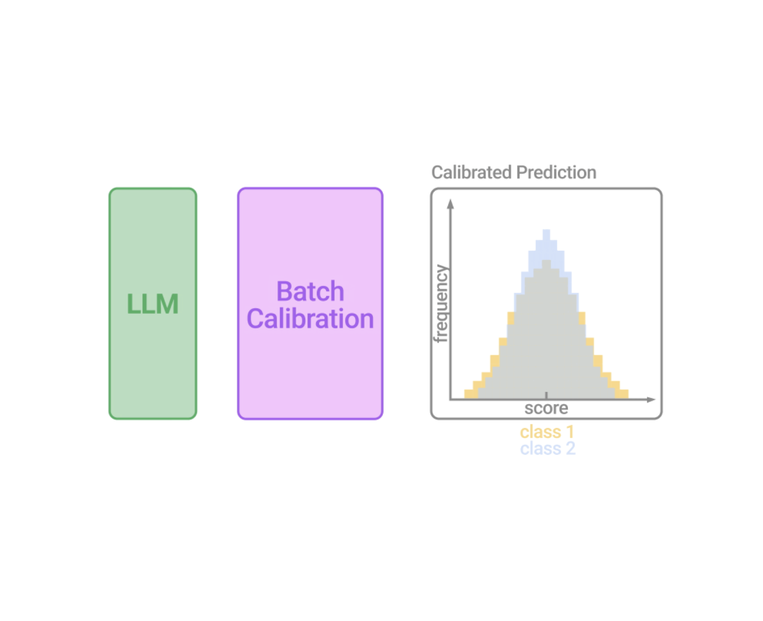
Inspired by the previous discussions, we designed BC to be a zero-shot, inference-only and generalizable calibration technique with negligible computation cost. We argue that the most critical component for calibration is to accurately estimate the contextual bias. We, therefore, opt for a linear decision boundary for its robustness, and instead of relying on content-free inputs, we propose to estimate the contextual bias for each class from a batch in a content-based manner by marginalizing the output score over all samples within the batch, which is equivalent to measuring the mean score for each class (visualized below).

We then obtain the calibrated probability by dividing the output probability over the contextual prior, which is equivalent to aligning the log-probability (LLM scores) distribution to the estimated mean of each class. It is noteworthy that because it requires no additional inputs to estimate the bias, this BC procedure is zero-shot, only involves unlabeled test samples, and incurs negligible computation costs. We may either compute the contextual bias once all test samples are seen, or alternatively, in an on-the-fly manner that dynamically processes the outputs. To do so, we may use a running estimate of the contextual bias for BC, thereby allowing BC's calibration term to be estimated from a small number of mini-batches that is subsequently stabilized when more mini-batches arrive.

Illustration of Batch Calibration (BC). Batches of demonstrations with in-context examples and test samples are passed into the LLM. Due to sources of implicit bias in the context, the score distribution from the LLM becomes biased. BC is a modular and adaptable layer option appended to the output of the LLM that generates calibrated scores (visualized for illustration only).

Experiment design

For natural language tasks, we conduct experiments on 13 more diverse and challenging classification tasks, including the standard GLUE and SuperGLUE datasets. This is in contrast to previous works that only report on relatively simple single-sentence classification tasks.. For image classification tasks, we include SVHN, EuroSAT, and CLEVR. We conduct experiments mainly on the state-of-the-art PaLM 2 with size variants PaLM 2-S, PaLM 2-M, and PaLM 2-L. For VLMs, we report the results on CLIP ViT-B/16.


Results

Notably, BC consistently outperforms ICL, yielding a significant performance enhancement of 8% and 6% on small and large variants of PaLM 2, respectively. This shows that the BC implementation successfully mitigates the contextual bias from the in-context examples and unleashes the full potential of LLM in efficient learning and quick adaptation to new tasks. In addition, BC improves over the state-of-the-art prototypical calibration (PC) baseline by 6% on PaLM 2-S, and surpasses the competitive contextual calibration (CC) baseline by another 3% on average on PaLM 2-L. Specifically, BC is a generalizable and cheaper technique across all evaluated tasks, delivering stable performance improvement, whereas previous baselines exhibit varying degrees of performance across tasks.

Batch Calibration (BC) achieves the best performance on 1-shot ICL over calibration baselines: contextual calibration (CC), domain-context calibration (DC), and prototypical calibration (PC) on an average of 13 NLP tasks on PaLM 2 and outperforms the zero-shot CLIP on image tasks.

We analyze the performance of BC by varying the number of ICL shots from 0 to 4, and BC again outperforms all baseline methods. We also observe an overall trend for improved performance when more shots are available, where BC demonstrates the best stability.

The ICL performance on various calibration techniques over the number of ICL shots on PaLM 2-S. We compare BC with the uncalibrated ICL, contextual calibration (CC), domain-context calibration (DC), and prototypical calibration (PC) baselines.

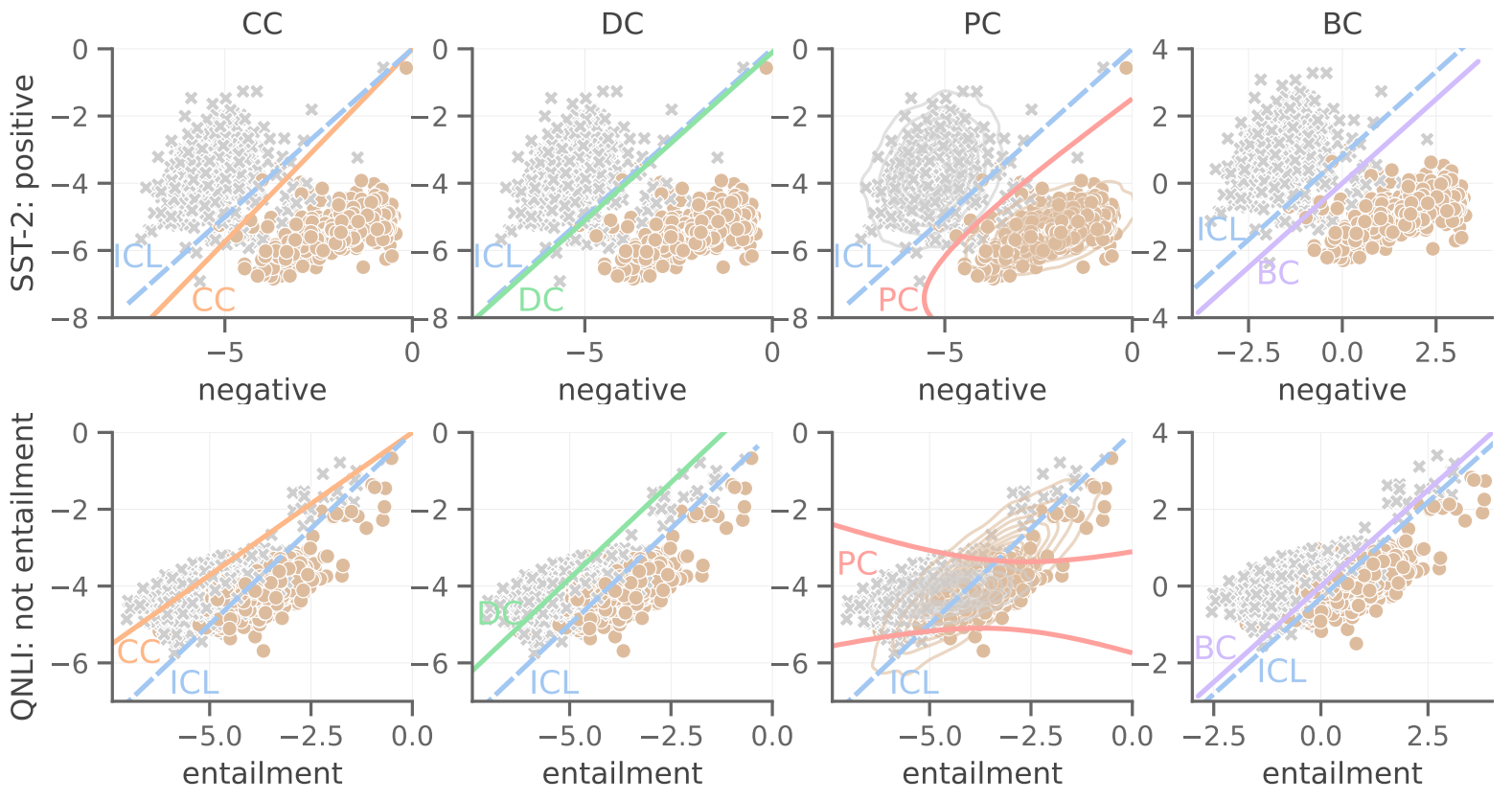
We further visualize the decision boundaries of uncalibrated ICL after applying existing calibration methods and the proposed BC. We show success and failure cases for each baseline method, whereas BC is consistently effective.

Visualization of the decision boundaries of uncalibrated ICL, and after applying existing calibration methods and the proposed BC in representative binary classification tasks of SST-2 (top row) and QNLI (bottom row) on 1-shot PaLM 2-S. Each axis indicates the LLM score on the defined label.

Robustness and ablation studies

We analyze the robustness of BC with respect to common prompt engineering design choices that were previously shown to significantly affect LLM performance: choices and orders of in-context examples, the prompt template for ICL, and the label space. First, we find that BC is more robust to ICL choices and can mostly achieve the same performance with different ICL examples. Additionally, given a single set of ICL shots, altering the order between each ICL example has minimal impact on the BC performance. Furthermore, we analyze the robustness of BC under 10 designs of prompt templates, where BC shows consistent improvement over the ICL baseline. Therefore, though BC improves performance, a well-designed template can further enhance the performance of BC. Lastly, we examine the robustness of BC to variations in label space designs (see appendix in our paper). Remarkably, even when employing unconventional choices such as emoji pairs as labels, leading to dramatic oscillations of ICL performance, BC largely recovers performance. This observation demonstrates that BC increases the robustness of LLM predictions under common prompt design choices and makes prompt engineering easier.

Batch Calibration makes prompt engineering easier while being data-efficient. Data are visualized as a standard box plot, which illustrates values for the median, first and third quartiles, and minimum and maximum.

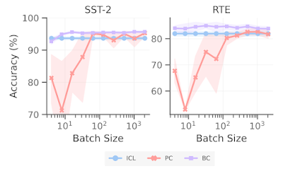
Moreover, we study the impact of batch size on the performance of BC. In contrast to PC, which also leverages an unlabeled estimate set, BC is remarkably more sample efficient, achieving a strong performance with only around 10 unlabeled samples, whereas PC requires more than 500 unlabeled samples before its performance stabilizes.

Batch Calibration makes prompt engineering easier while being insensitive to the batch size.

Conclusion

We first revisit previous calibration methods while addressing two critical research questions from an interpretation of decision boundaries, revealing their failure cases and deficiencies. We then propose Batch Calibration, a zero-shot and inference-only calibration technique. While methodologically simple and easy to implement with negligible computation cost, we show that BC scales from a language-only setup to the vision-language context, achieving state-of-the-art performance in both modalities. BC significantly improves the robustness of LLMs with respect to prompt designs, and we expect easy prompt engineering with BC.


Acknowledgements

This work was conducted by Han Zhou, Xingchen Wan, Lev Proleev, Diana Mincu, Jilin Chen, Katherine Heller, Subhrajit Roy. We would like to thank Mohammad Havaei and other colleagues at Google Research for their discussion and feedback.

Source: Google AI Blog


Developing industrial use cases for physical simulation on future error-corrected quantum computers

If you’ve paid attention to the quantum computing space, you’ve heard the claim that in the future, quantum computers will solve certain problems exponentially more efficiently than classical computers can. They have the potential to transform many industries, from pharmaceuticals to energy.

For the most part, these claims have rested on arguments about the asymptotic scaling of algorithms as the problem size approaches infinity, but this tells us very little about the practical performance of quantum computers for finite-sized problems. We want to be more concrete: Exactly which problems are quantum computers more suited to tackle than their classical counterparts, and exactly what quantum algorithms could we run to solve these problems? Once we’ve designed an algorithm, we can go beyond analysis based on asymptotic scaling — we can determine the actual resources required to compile and run the algorithm on a quantum computer, and how that compares to a classical computation.

Over the last few years, Google Quantum AI has collaborated with industry and academic partners to assess the prospects for quantum simulation to revolutionize specific technologies and perform concrete analyses of the resource requirements. In 2022, we developed quantum algorithms to analyze the chemistry of an important enzyme family called cytochrome P450. Then, in our paper released this fall, we demonstrated how to use a quantum computer to study sustainable alternatives to cobalt for use in lithium ion batteries. And most recently, as we report in a preprint titled “Quantum computation of stopping power for inertial fusion target design,” we’ve found a new application in modeling the properties of materials in inertial confinement fusion experiments, such as those at the National Ignition Facility (NIF) at Lawrence Livermore National Laboratory, which recently made headlines for a breakthrough in nuclear fusion.

Below, we describe these three industrially relevant applications for simulations with quantum computers. While running the algorithms will require an error-corrected quantum computer, which is still years away, working on this now will ensure that we are ready with efficient quantum algorithms when such a quantum computer is built. Already, our work has reduced the cost of compiling and running the algorithms significantly, as we have reported in the past. Our work is essential for demonstrating the potential of quantum computing, but it also provides our hardware team with target specifications for the number of qubits and time needed to run useful quantum algorithms in the future.


Application 1: The CYP450 mechanism

The pharmaceutical industry is often touted as a field ripe for discovery using quantum computers. But concrete examples of such potential applications are few and far between. Working with collaborators at the pharmaceutical company Boehringer Ingelheim, our partners at the startup QSimulate, and academic colleagues at Columbia University, we explored one example in the 2022 PNAS article, “Reliably assessing the electronic structure of cytochrome P450 on today’s classical computers and tomorrow’s quantum computers”.

Cytochrome P450 is an enzyme family naturally found in humans that helps us metabolize drugs. It excels at its job: more than 70% of all drug metabolism is performed by enzymes of the P450 family. The enzymes work by oxidizing the drug — a process that depends on complex correlations between electrons. The details of the interactions are too complicated for scientists to know a priori how effective the enzyme will be on a particular drug.

In the paper, we showed how a quantum computer could approach this problem. The CYP450 metabolic process is a complex chain of reactions with many intermediate changes in the electronic structure of the enzymes throughout. We first use state-of-the-art classical methods to determine the resources required to simulate this problem on a classical computer. Then we imagine implementing a phase-estimation algorithm — which is needed to compute the ground-state energies of the relevant electronic configurations throughout the reaction chain — on a surface-code error-corrected quantum computer.

With a quantum computer, we could follow the chain of changing electronic structure with greater accuracy and fewer resources. In fact, we find that the higher accuracy offered by a quantum computer is needed to correctly resolve the chemistry in this system, so not only will a quantum computer be better, it will be necessary. And as the system size gets bigger, i.e., the more quantum energy levels we include in the simulation, the more the quantum computer wins over the classical computer. Ultimately, we show that a few million physical qubits would be required to reach quantum advantage for this problem.

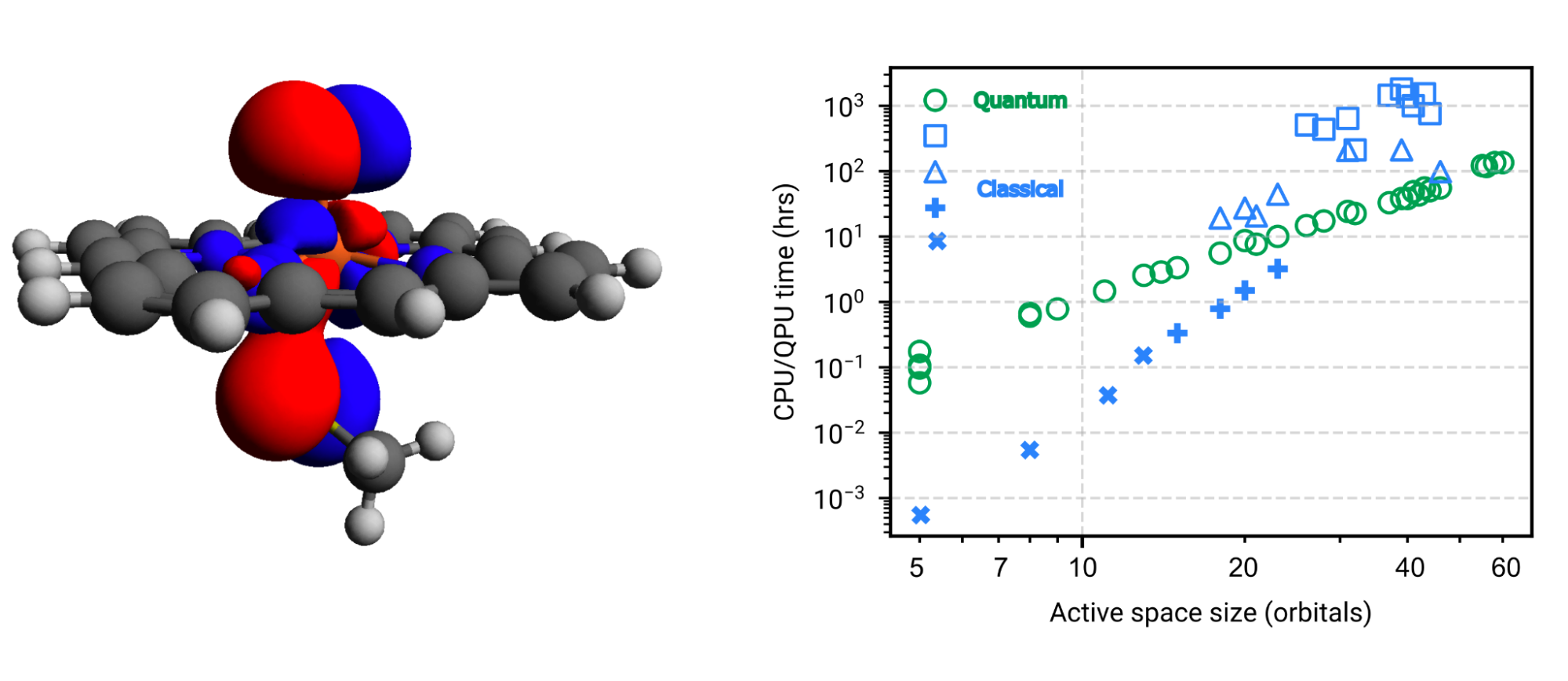
Left: Example of an electron orbital (red and blue) of a CYP enzyme. More than 60 such orbitals are required to model the CYP system. Right: Comparison of actual runtime (CPU) of various classical techniques (blue) to hypothetical runtime (QPU) of a quantum algorithm (green). The lower slope of the quantum algorithm demonstrates the favorable asymptotic scaling over classical methods. Already at about 20-30 orbitals, we see a crossover to the regime where a quantum algorithm would be more efficient than classical methods.

Application 2: Lithium-ion batteries

Lithium-ion batteries rely on the electrochemical potential difference between two lithium containing materials. One material used today for the cathodes of Li-ion batteries is LiCoO2. Unfortunately, it has drawbacks from a manufacturing perspective. Cobalt mining is expensive, destructive to the environment, and often utilizes unsafe or abusive labor practices. Consequently, many in the field are interested in alternatives to cobalt for lithium-ion cathodes.

In the 1990’s, researchers discovered that nickel could replace cobalt to form LiNiO2 (called “lithium nickel oxide” or “LNO”) for cathodes. While pure LNO was found to be unstable in production, many cathode materials used in the automotive industry today use a high fraction of nickel and hence, resemble LNO. Despite its applications to industry, however, not all of the chemical properties of LNO are understood — even the properties of its ground state remains a subject of debate.

In our recent paper, “Fault tolerant quantum simulation of materials using Bloch orbitals,” we worked with the chemical company, BASF, the molecular modeling startup, QSimulate, and collaborators at Macquarie University in Australia to develop techniques to perform quantum simulations on systems with periodic, regularly spaced atomic structure, such as LNO. We then applied these techniques to design algorithms to study the relative energies of a few different candidate structures of LNO. With classical computers, high accuracy simulations of the quantum wavefunction are considered too expensive to perform. In our work, we found that a quantum computer would need tens of millions of physical qubits to calculate the energies of each of the four candidate ground-state LNO structures. This is out of reach of the first error-corrected quantum computers, but we expect this number to come down with future algorithmic improvements.

Four candidate structures of LNO. In the paper, we consider the resources required to compare the energies of these structures in order to find the ground state of LNO.

Application 3: Fusion reactor dynamics

In our third and most recent example, we collaborated with theorists at Sandia National Laboratories and our Macquarie University collaborators to put our hypothetical quantum computer to the task of simulating dynamics of charged particles in the extreme conditions typical of inertial confinement fusion (ICF) experiments, like those at the National Ignition Facility. In those experiments, high-intensity lasers are focused into a metallic cavity (hohlraum) that holds a target capsule consisting of an ablator surrounding deuterium–tritium fuel. When the lasers heat the inside of the hohlraum, its walls radiate x-rays that compress the capsule, heating the deuterium and tritium inside to 10s of millions of Kelvin. This allows the nucleons in the fuel to overcome their mutual electrostatic repulsion and start fusing into helium nuclei, also called alpha particles.

Simulations of these experiments are computationally demanding and rely on models of material properties that are themselves uncertain. Even testing these models, using methods similar to those in quantum chemistry, is extremely computationally expensive. In some cases, such test calculations have consumed >100 million CPU hours. One of the most expensive and least accurate aspects of the simulation is the dynamics of the plasma prior to the sustained fusion stage (>10s of millions of Kelvin), when parts of the capsule and fuel are a more balmy 100k Kelvin. In this “warm dense matter” regime, quantum correlations play a larger role in the behavior of the system than in the “hot dense matter” regime when sustained fusion takes place.

In our new preprint, “Quantum computation of stopping power for inertial fusion target design”, we present a quantum algorithm to compute the so-called “stopping power” of the warm dense matter in a nuclear fusion experiment. The stopping power is the rate at which a high energy alpha particle slows down due to Coulomb interactions with the surrounding plasma. Understanding the stopping power of the system is vital for optimizing the efficiency of the reactor. As the alpha particle is slowed by the plasma around it, it transfers its energy to the plasma, heating it up. This self-heating process is the mechanism by which fusion reactions sustain the burning plasma. Detailed modeling of this process will help inform future reactor designs.

We estimate that the quantum algorithm needed to calculate the stopping power would require resources somewhere between the P450 application and the battery application. But since this is the first case study on first-principles dynamics (or any application at finite temperature), such estimates are just a starting point and we again expect to find algorithmic improvements to bring this cost down in the future. Despite this uncertainty, it is still certainly better than the classical alternative, for which the only tractable approaches for these simulations are mean-field methods. While these methods incur unknown systematic errors when describing the physics of these systems, they are currently the only meaningful means of performing such simulations.

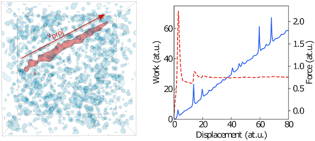
Left: A projectile (red) passing through a medium (blue) with initial velocity vproj. Right: To calculate the stopping power, we monitor the energy transfer between the projectile and the medium (blue solid line) and determine its average slope (red dashed line).

Discussion and conclusion

The examples described above are just three of a large and growing body of concrete applications for a future error-corrected quantum computer in simulating physical systems. This line of research helps us understand the classes of problems that will most benefit from the power of quantum computing. In particular, the last example is distinct from the other two in that it is simulating a dynamical system. In contrast to the other problems, which focus on finding the lowest energy, static ground state of a quantum system, quantum dynamics is concerned with how a quantum system changes over time. Since quantum computers are inherently dynamic — the qubit states evolve and change as each operation is performed — they are particularly well suited to solving these kinds of problems. Together with collaborators at Columbia, Harvard, Sandia National Laboratories and Macquarie University in Australia we recently published a paper in Nature Communications demonstrating that quantum algorithms for simulating electron dynamics can be more efficient even than approximate, “mean-field” classical calculations, while simultaneously offering much higher accuracy.

Developing and improving algorithms today prepares us to take full advantage of them when an error-corrected quantum computer is eventually realized. Just as in the classical computing case, we expect improvements at every level of the quantum computing stack to further lower the resource requirements. But this first step helps separate hyperbole from genuine applications amenable to quantum computational speedups.


Acknowledgements

We would like to thank Katie McCormick, our Quantum Science Communicator, for helping to write this blog post.

Source: Google AI Blog


SANPO: A Scene understanding, Accessibility, Navigation, Pathfinding, & Obstacle avoidance dataset

As most people navigate their everyday world, they process visual input from the environment using an eye-level perspective. Unlike robots and self-driving cars, people don't have any "out-of-body" sensors to help guide them. Instead, a person’s sensory input is completely "egocentric", or "from the self." This also applies to new technologies that understand the world around us from a human-like perspective, e.g., robots navigating through unknown buildings, AR glasses that highlight objects, or assistive technology to help people run independently.

In computer vision, scene understanding is the subfield that studies how visible objects relate to the scene's 3D structure and layout by focusing on the spatial, functional, and semantic relationships between objects and their environment. For example, autonomous drivers must understand the 3D structure of the road, sidewalks, and surrounding buildings while identifying and recognizing street signs and stop lights, a task made easier with 3D data from a special laser scanner mounted on the top of the car rather than 2D images from the driver’s perspective. Robots navigating a park must understand where the path is and what obstacles might interfere, which is simplified with a map of their surroundings and GPS positioning data. Finally, AR glasses that help users find their way need to understand where the user is and what they are looking at.
The computer vision community typically studies scene understanding tasks in contexts like self-driving, where many other sensors (GPS, wheel positioning, maps, etc.) beyond egocentric imagery are available. Yet most datasets in this space do not focus exclusively on egocentric data, so they are less applicable to human-centered navigation tasks. While there are plenty of self-driving focused scene understanding datasets, they have limited generalization to egocentric human scene understanding. A comprehensive human egocentric dataset would help build systems for related applications and serve as a challenging benchmark for the scene understanding community.

To that end, we present the Scene understanding, Accessibility, Navigation, Pathfinding, Obstacle avoidance dataset, or SANPO (also the Japanese word for ”brisk stroll”), a multi-attribute video dataset for outdoor human egocentric scene understanding. The dataset consists of real world data and synthetic data, which we call SANPO-Real and SANPO-Synthetic, respectively. It supports a wide variety of dense prediction tasks, is challenging for current models, and includes real and synthetic data with depth maps and video panoptic masks in which each pixel is assigned a semantic class label (and for some semantic classes, each pixel is also assigned a semantic instance ID that uniquely identifies that object in the scene). The real dataset covers diverse environments and has videos from two stereo cameras to support multi-view methods, including 11.4 hours captured at 15 frames per second (FPS) with dense annotations. Researchers can download and use SANPO here.

3D scene of a real session built using the provided annotations (segmentation, depth and camera positions). The top center video shows the depth map, and the top right shows the RGB or semantic annotations.

SANPO-Real

SANPO-Real is a multiview video dataset containing 701 sessions recorded with two stereo cameras: a head-mounted ZED Mini and a chest-mounted ZED-2i. That’s four RGB streams per session at 15 FPS. 597 sessions are recorded at a resolution of 2208x1242 pixels, and the remainder are recorded at a resolution of 1920x1080 pixels. Each session is approximately 30 seconds long, and the recorded videos are rectified using Zed software and saved in a lossless format. Each session has high-level attribute annotations, camera pose trajectories, dense depth maps from CREStereo, and sparse depth maps provided by the Zed SDK. A subset of sessions have temporally consistent panoptic segmentation annotations of each instance.

The SANPO data collection system for collecting real-world data. Right: (i) a backpack with ZED 2i and ZED Mini cameras for data collection (bottom), (ii) the inside of the backpack showing the ZED box and battery pack mounted on a 3D printed container (middle), and (iii) an Android app showing the live feed from the ZED cameras (top). Left: The chest-mounted ZED-2i has a stereo baseline of 12cm with a 2.1mm focal length, and the head-mounted ZED Mini has a baseline of 6.3cm with a 2.1mm focal length.

Temporally consistent panoptic segmentation annotation protocol

SANPO includes thirty different class labels, including various surfaces (road, sidewalk, curb, etc.), fences (guard rails, walls,, gates), obstacles (poles, bike racks, trees), and creatures (pedestrians, riders, animals). Gathering high-quality annotations for these classes is an enormous challenge. To provide temporally consistent panoptic segmentation annotation we divide each video into 30-second sub-videos and annotate every fifth frame (90 frames per sub-video), using a cascaded annotation protocol. At each stage, we ask annotators to draw borders around five mutually exclusive labels at a time. We send the same image to different annotators with as many stages as it takes to collect masks until all labels are assigned, with annotations from previous subsets frozen and shown to the annotator. We use AOT, a machine learning model that reduces annotation effort by giving annotators automatic masks from which to start, taken from previous frames during the annotation process. AOT also infers segmentation annotations for intermediate frames using the manually annotated preceding and following frames. Overall, this approach reduces annotation time, improves boundary precision, and ensures temporally consistent annotations for up to 30 seconds.

Temporally consistent panoptic segmentation annotations. The segmentation mask’s title indicates whether it was manually annotated or AOT propagated.

SANPO-Synthetic

Real-world data has imperfect ground truth labels due to hardware, algorithms, and human mistakes, whereas synthetic data has near-perfect ground truth and can be customized. We partnered with Parallel Domain, a company specializing in lifelike synthetic data generation, to create SANPO-Synthetic, a high-quality synthetic dataset to supplement SANPO-Real. Parallel Domain is skilled at creating handcrafted synthetic environments and data for machine learning applications. Thanks to their work, SANPO-Synthetic matches real-world capture conditions with camera parameters, placement, and scenery.

3D scene of a synthetic session built using the provided annotations (segmentation, depth and odometry). The top center video shows the depth map, and the top right shows the RGB or semantic annotations.

SANPO-Synthetic is a high quality video dataset, handcrafted to match real world scenarios. It contains 1961 sessions recorded using virtualized Zed cameras, evenly split between chest-mounted and head-mounted positions and calibrations. These videos are monocular, recorded from the left lens only. These sessions vary in length and FPS (5, 14.28, and 33.33) for a mix of temporal resolution / length tradeoffs, and are saved in a lossless format. All the sessions have precise camera pose trajectories, dense pixel accurate depth maps and temporally consistent panoptic segmentation masks.

SANPO-Synthetic data has pixel-perfect annotations, even for small and distant instances. This helps develop challenging datasets that mimic the complexity of real-world scenes. SANPO-Synthetic and SANPO-Real are also drop-in replacements for each other, so researchers can study domain transfer tasks or use synthetic data during training with few domain-specific assumptions.

An even sampling of real and synthetic scenes.

Statistics

Semantic classes

We designed our SANPO taxonomy: i) with human egocentric navigation in mind, ii) with the goal of being reasonably easy to annotate, and iii) to be as close as possible to the existing segmentation taxonomies. Though built with human egocentric navigation in mind, it can be easily mapped or extended to other human egocentric scene understanding applications. Both SANPO-Real and SANPO-Synthetic feature a wide variety of objects one would expect in egocentric obstacle detection data, such as roads, buildings, fences, and trees. SANPO-Synthetic includes a broad distribution of hand-modeled objects, while SANPO-Real features more “long-tailed” classes that appear infrequently in images, such as gates, bus stops, or animals.

Distribution of images across the classes in the SANPO taxonomy.

Instance masks

SANPO-Synthetic and a portion of SANPO-Real are also annotated with panoptic instance masks, which assign each pixel to a class and instance ID. Because it is generally human-labeled, SANPO-Real has a large number of frames with generally less than 20 instances per frame. Similarly, SANPO-Synthetic’s virtual environment offers pixel-accurate segmentation of most unique objects in the scene. This means that synthetic images frequently feature many more instances within each frame.

When considering per-frame instance counts, synthetic data frequently features many more instances per frame than the labeled portions of SANPO-Real.

Comparison to other datasets

We compare SANPO to other important video datasets in this field, including SCAND, MuSoHu, Ego4D, VIPSeg, and Waymo Open. Some of these are intended for robot navigation (SCAND) or autonomous driving (Waymo) tasks. Across these datasets, only Waymo Open and SANPO have both panoptic segmentations and depth maps, and only SANPO has both real and synthetic data.

Comparison to other video datasets. For stereo vs mono video, datasets marked with ★ have stereo video for all scenes and those marked ☆ provide stereo video for a subset. For depth maps, ★ indicates dense depth while ☆ represents sparse depth, e.g., from a lower-resolution LIDAR scanner.

Conclusion and future work

We present SANPO, a large-scale and challenging video dataset for human egocentric scene understanding, which includes real and synthetic samples with dense prediction annotations. We hope SANPO will help researchers build visual navigation systems for the visually impaired and advance visual scene understanding. Additional details are available in the preprint and on the SANPO dataset GitHub repository.


Acknowledgements

This dataset was the outcome of hard work of many individuals from various teams within Google and our external partner, Parallel Domain.

Core Team: Mikhail Sirotenko, Dave Hawkey, Sagar Waghmare, Kimberly Wilber, Xuan Yang, Matthew Wilson

Parallel Domain: Stuart Park, Alan Doucet, Alex Valence-Lanoue, & Lars Pandikow.

We would also like to thank following team members: Hartwig Adam, Huisheng Wang, Lucian Ionita, Nitesh Bharadwaj, Suqi Liu, Stephanie Debats, Cattalyya Nuengsigkapian, Astuti Sharma, Alina Kuznetsova, Stefano Pellegrini, Yiwen Luo, Lily Pagan, Maxine Deines, Alex Siegman, Maura O’Brien, Rachel Stigler, Bobby Tran, Supinder Tohra, Umesh Vashisht, Sudhindra Kopalle, Reet Bhatia.

Source: Google AI Blog


Scalable spherical CNNs for scientific applications

Typical deep learning models for computer vision, like convolutional neural networks (CNNs) and vision transformers (ViT), process signals assuming planar (flat) spaces. For example, digital images are represented as a grid of pixels on a plane. However, this type of data makes up only a fraction of the data we encounter in scientific applications. Variables sampled from the Earth's atmosphere, like temperature and humidity, are naturally represented on the sphere. Some kinds of cosmological data and panoramic photos are also spherical signals, and are better treated as such.

Using methods designed for planar images to process spherical signals is problematic for a couple of reasons. First, there is a sampling problem, i.e., there is no way of defining uniform grids on the sphere, which are needed for planar CNNs and ViTs, without heavy distortion.

When projecting the sphere into a plane, the patch represented by the red circle is heavily distorted near the poles. This sampling problem hurts the accuracy of conventional CNNs and ViTs on spherical inputs.

Second, signals and local patterns on the sphere are often complicated by rotations, so models need a way to address that. We would like equivariance to 3D rotations, which ensures that learned features follow the rotations of the input. This leads to better utilization of the model parameters and allows training with less data. Equivariance to 3D rotations is also useful in most settings where inputs don’t have a preferred orientation, such as 3D shapes and molecules.

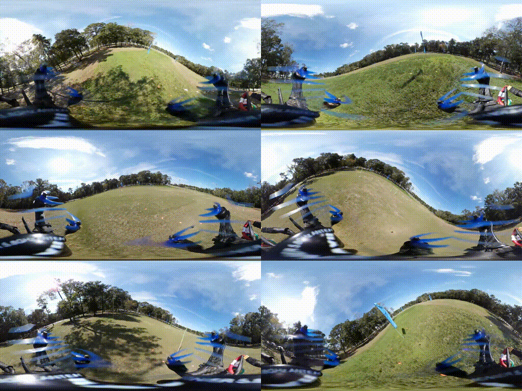
Drone racing with panoramic cameras. Here the sharp turns result in large 3D rotations of the spherical image. We would like our models to be robust to such rotations. Source: https://www.youtube.com/watch?v=_J7qXbbXY80 (licensed under CC BY)
In the atmosphere, it is common to see similar patterns appearing at different positions and orientations. We would like our models to share parameters to recognize these patterns.

With the above challenges in mind, in “Scaling Spherical CNNs”, presented at ICML 2023, we introduce an open-source library in JAX for deep learning on spherical surfaces. We demonstrate how applications of this library match or surpass state-of-the-art performance on weather forecasting and molecular property prediction benchmarks, tasks that are typically addressed with transformers and graph neural networks.


Background on spherical CNNs

Spherical CNNs solve both the problems of sampling and of robustness to rotation by leveraging spherical convolution and cross-correlation operations, which are typically computed via generalized Fourier transforms. For planar surfaces, however, convolution with small filters is faster, because it can be performed on regular grids without using Fourier transforms. The higher computational cost for spherical inputs has so far restricted the application of spherical CNNs to small models and datasets and low resolution datasets.


Our contributions

We have implemented the spherical convolutions from spin-weighted spherical CNNs in JAX with a focus on speed, and have enabled distributed training over a large number of TPUs using data parallelism. We also introduced a new phase collapse activation and spectral batch normalization layer, and a new residual block that improves accuracy and efficiency, which allows training more accurate models up to 100x larger than before. We apply these new models on molecular property regression and weather forecasting.

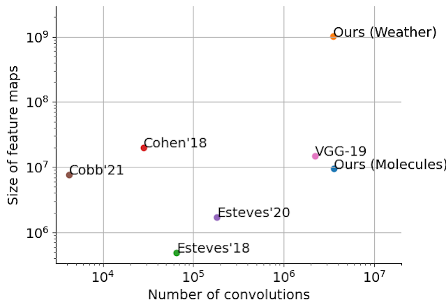
We scale spherical CNNs by up to two orders of magnitude in terms of feature sizes and model capacity, compared to the literature: Cohen’18Esteves’18Esteves’20, and Cobb’21VGG-19 is included as a conventional CNN reference. Our largest model for weather forecasting has 256 x 256 x 78 inputs and outputs, and runs 96 convolutional layers during training with a lowest internal resolution of 128 x 128 x 256.

Molecular property regression

Predicting properties of molecules has applications in drug discovery, where the goal is to quickly screen numerous molecules in search of those with desirable properties. Similar models may also be relevant in the design of drugs targeting the interaction between proteins. Current methods in computational or experimental quantum chemistry are expensive, which motivates the use of machine learning.

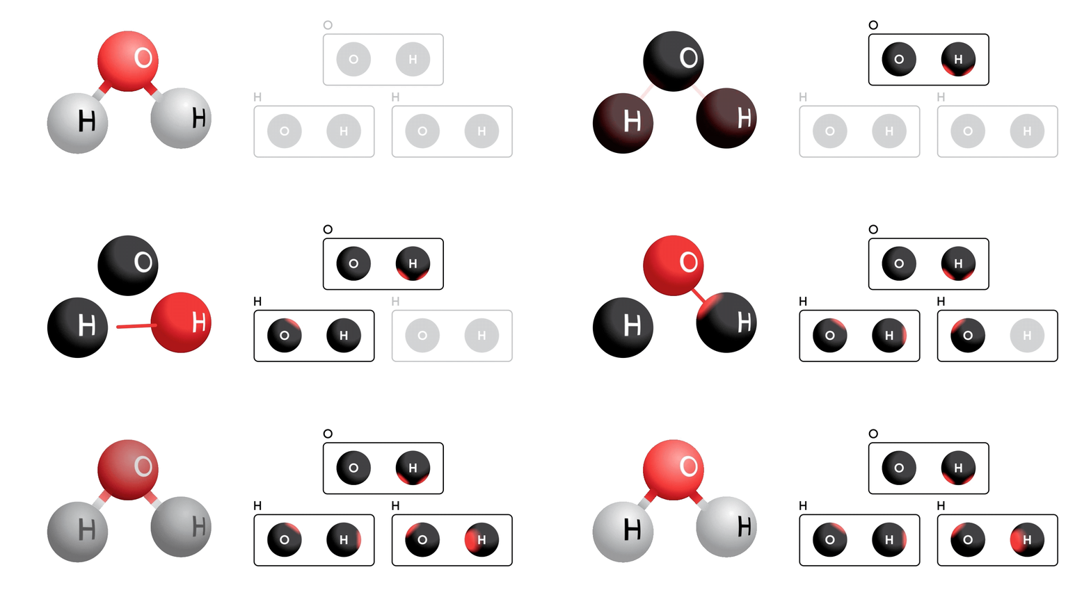
Molecules can be represented by a set of atoms and their positions in 3D space; rotations of the molecule change the positions but not the molecular properties. This motivates the application of spherical CNNs because of their rotation equivariance. However, molecules are not defined as signals on the sphere so the first step is to map them to a set of spherical functions. We do so by leveraging physics-based interactions between the atoms of the molecule.

Each atom is represented by a set of spherical signals accumulating physical interactions with other atoms of each type (shown in the three panels on the right). For example, the oxygen atom (O; top panel) has a channel for oxygen (indicated by the sphere labeled “O” on the left) and hydrogen (“H”, right). The accumulated Coulomb forces on the oxygen atom with respect to the two hydrogen atoms is indicated by the red shaded regions on the bottom of the sphere labeled “H”. Because the oxygen atom contributes no forces to itself, the “O” sphere is uniform. We include extra channels for the Van der Waals forces.

Spherical CNNs are applied to each atom's features, and results are later combined to produce the property predictions. This results in state-of-the art performance in most properties as typically evaluated in the QM9 benchmark:

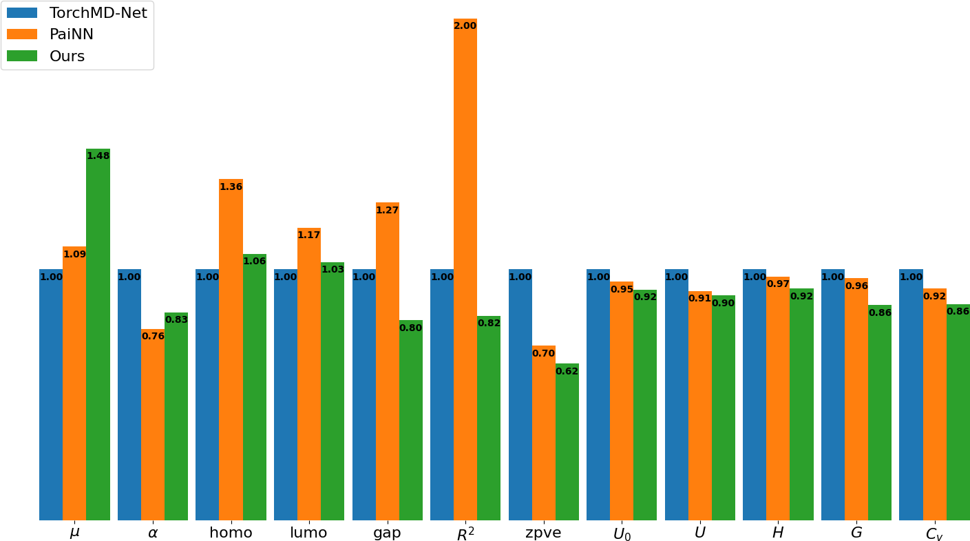
Error comparison against the state-of-the-art on 12 properties of QM9 (see the dataset paper for details). We show TorchMD-Net and PaiNN results, normalizing TorchMD-Net errors to 1.0 (lower is better). Our model, shown in green, outperforms the baselines in most targets.

Weather forecasting

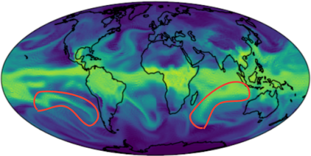
Accurate climate forecasts serve as invaluable tools for providing timely warnings of extreme weather events, enabling effective water resource management, and guiding informed infrastructure planning. In a world increasingly threatened by climate disasters, there is an urgency to deliver forecasts much faster and more accurately over a longer time horizon than general circulation models. Forecasting models will also be important for predicting the safety and effectiveness of efforts intended to combat climate change, such as climate interventions. The current state-of-the-art uses costly numerical models based on fluid dynamics and thermodynamics, which tend to drift after a few days.

Given these challenges, there is an urgency for machine learning researchers to address climate forecasting problems, as data-driven techniques have the potential of both reducing the computational cost and improving long range accuracy. Spherical CNNs are suitable for this task since atmospheric data is natively presented on the sphere. They can also efficiently handle repeating patterns at different positions and orientations that are common in such data.

We apply our models to several weather forecasting benchmarks and outperform or match neural weather models based on conventional CNNs (specifically, 1, 2, and 3). Below we show results in a test setting where the model takes a number of atmospheric variables as input and predicts their values six hours ahead. The model is then iteratively applied on its own predictions to produce longer forecasts. During training, the model predicts up to three days ahead, and is evaluated up to five days. Keisler proposed a graph neural network for this task, but we show that spherical CNNs can match the GNN accuracy in the same setting.

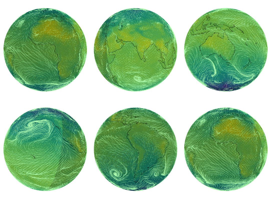
Iterative weather forecasting up to five days (120h) ahead with spherical CNNs. The animations show the specific humidity forecast at a given pressure and its error.
Wind speed and temperature forecasts with spherical CNNs.

Additional resources

Our JAX library for efficient spherical CNNs is now available. We have shown applications to molecular property regression and weather forecasting, and we believe the library will be helpful in other scientific applications, as well as in computer vision and 3D vision.

Weather forecasting is an active area of research at Google with the goal of building more accurate and robust models — like Graphcast, a recent ML-based mid-range forecasting model — and to build tools that enable further advancement across the research community, such as the recently released WeatherBench 2.


Acknowledgements

This work was done in collaboration with Jean-Jacques Slotine, and is based on previous collaborations with Kostas Daniilidis and Christine Allen-Blanchette. We thank Stephan Hoyer, Stephan Rasp, and Ignacio Lopez-Gomez for helping with data processing and evaluation, and Fei Sha, Vivian Yang, Anudhyan Boral, Leonardo Zepeda-Núñez, and Avram Hershko for suggestions and discussions. We are thankful to Michael Riley and Corinna Cortes for supporting and encouraging this project.

Source: Google AI Blog


Google at ICCV 2023

Google is proud to be a Platinum Sponsor of the International Conference on Computer Vision (ICCV 2023), a premier annual conference, which is being held this week in Paris, France. As a leader in computer vision research, Google has a strong presence at this year’s conference with 60 accepted papers and active involvement in 27 workshops and tutorials. Google is also proud to be a Platinum Sponsor for the LatinX in CV workshop. We look forward to sharing some of our extensive computer vision research and expanding our partnership with the broader research community.

Attending ICCV 2023? We hope you’ll visit the Google booth to chat with researchers who are actively pursuing the latest innovations in computer vision, and check out some of the scheduled booth activities (e.g., demos and Q&A sessions listed below). Visit the @GoogleAI Twitter account to find out more about the Google booth activities at ICCV 2023.

Take a look below to learn more about the Google research being presented at ICCV 2023 (Google affiliations in bold).


Board and Organizing Committee

General Chair: Cordelia Schmid
Finance Chair: Ramin Zabih
Industrial Relations Chair: Rahul Sukthankar
Publicity and Social Media Co-Chair: Boqing Gong


Google Research booth activities

Title: ImagenThings: Instant Personalized Image-to-Image Generation
Presenters: Xuhui Jia, Suraj Kothawade
Wednesday, October 4th at 12:30 PM CEST

Title: Open Images V7 (paper, dataset, blog post)
Presenters: Rodrigo Benenson, Jasper Uijlings, Jordi Pont-Tuset
Wednesday, October 4th at 3:30 PM CEST

Title: AI4Design (paper)
Presenters: Andrew Marmon, Peggy Chi, C.K. Ng
Thursday, October 5th at 10:30 AM CEST

Title: Preface: A Data-driven Volumetric Prior for Few-shot Ultra High-resolution Face Synthesis
Presenters: Marcel Bühler, Kripasindhu Sarkar
Thursday, October 5th at 12:30 PM CEST

Title: WHOOPS! A Vision-and-Language Benchmark of Synthetic and Compositional Images
Presenters: Yonatan Bitton
Thursday, October 5th at 1:00 PM CEST

Title: Image Search in Fact Check Explorer (blog post)
Presenters: Yair Alon, Avneesh Sud
Thursday, October 5th at 3:30 PM CEST

Title: UnLoc: A Unified Framework for Video Localization Tasks (paper)
Presenters: Arsha Nagrani, Xuehan Xiong
Friday, October 6th at 10:30 AM CEST

Title: Prompt-Tuning Latent Diffusion Models for Inverse Problems
Presenters: Hyungjin Chung
Friday, October 6th at 12:30 PM CEST

Title: Neural Implicit Representations for Real World Applications
Presenters: Federico Tombari, Fabian Manhardt, Marie-Julie Rakotosaona
Friday, October 6th at 3:30 PM CEST


Accepted papers

Multi-Modal Neural Radiance Field for Monocular Dense SLAM with a Light-Weight ToF Sensor
Xinyang Liu, Yijin Li, Yanbin Teng, Hujun Bao, Guofeng Zhang, Yinda Zhang, Zhaopeng Cui

ITI-GEN: Inclusive Text-to-Image Generation
Cheng Zhang, Xuanbai Chen, Siqi Chai, Chen Henry Wu, Dmitry Lagun, Thabo Beeler, Fernando De la Torre

ASIC: Aligning Sparse in-the-wild Image Collections
Kamal Gupta, Varun Jampani, Carlos Esteves, Abhinav Shrivastava, Ameesh Makadia, Noah Snavely, Abhishek Kar

VQ3D: Learning a 3D-Aware Generative Model on ImageNet
Kyle Sargent, Jing Yu Koh, Han Zhang, Huiwen Chang, Charles Herrmann, Pratul Srinivasan, Jiajun Wu, Deqing Sun

Open-domain Visual Entity Recognition: Towards Recognizing Millions of Wikipedia Entities
Hexiang Hu, Yi Luan, Yang Chen*, Urvashi Khandelwal, Mandar Joshi, Kenton Lee, Kristina Toutanova, Ming-Wei Chang

Sigmoid Loss for Language Image Pre-training
Xiaohua Zhai, Basil Mustafa, Alexander Kolesnikov, Lucas Beyer

Tracking Everything Everywhere All at Once
Qianqian Wang, Yen-Yu Chang, Ruojin Cai, Zhengqi Li, Bharath Hariharan, Aleksander Holynski, Noah Snavely

Zip-NeRF: Anti-Aliased Grid-Based Neural Radiance Fields
Jonathan T. Barron, Ben Mildenhall, Dor Verbin, Pratul P. Srinivasan, Peter Hedman

Delta Denoising Score
Amir Hertz*, Kfir Aberman, Daniel Cohen-Or*

DreamBooth3D: Subject-Driven Text-to-3D Generation
Amit Raj, Srinivas Kaza, Ben Poole, Michael Niemeyer, Nataniel Ruiz, Ben Mildenhall, Shiran Zada, Kfir Aberman, Michael Rubinstein, Jonathan Barron, Yuanzhen Li, Varun Jampani

Encyclopedic VQA: Visual Questions about Detailed Properties of Fine-grained Categories
Thomas Mensink, Jasper Uijlings, Lluis Castrejon, Arushi Goel*, Felipe Cadar*, Howard Zhou, Fei Sha, André Araujo, Vittorio Ferrari

GECCO: Geometrically-Conditioned Point Diffusion Models
Michał J. Tyszkiewicz, Pascal Fua, Eduard Trulls

Learning from Semantic Alignment between Unpaired Multiviews for Egocentric Video Recognition
Qitong Wang, Long Zhao, Liangzhe Yuan, Ting Liu, Xi Peng

Neural Microfacet Fields for Inverse Rendering
Alexander Mai, Dor Verbin, Falko Kuester, Sara Fridovich-Keil

Rosetta Neurons: Mining the Common Units in a Model Zoo
Amil Dravid, Yossi Gandelsman, Alexei A. Efros, Assaf Shocher

Teaching CLIP to Count to Ten
Roni Paiss*, Ariel Ephrat, Omer Tov, Shiran Zada, Inbar Mosseri, Michal Irani, Tali Dekel

Vox-E: Text-guided Voxel Editing of 3D Objects
Etai Sella, Gal Fiebelman, Peter Hedman, Hadar Averbuch-Elor

CC3D: Layout-Conditioned Generation of Compositional 3D Scenes
Sherwin Bahmani, Jeong Joon Park, Despoina Paschalidou, Xingguang Yan, Gordon Wetzstein, Leonidas Guibas, Andrea Tagliasacchi

Delving into Motion-Aware Matching for Monocular 3D Object Tracking
Kuan-Chih Huang, Ming-Hsuan Yang, Yi-Hsuan Tsai

Generative Multiplane Neural Radiance for 3D-Aware Image Generation
Amandeep Kumar, Ankan Kumar Bhunia, Sanath Narayan, Hisham Cholakkal, Rao Muhammad Anwer, Salman Khan, Ming-Hsuan Yang, Fahad Shahbaz Khan

M2T: Masking Transformers Twice for Faster Decoding
Fabian Mentzer, Eirikur Agustsson, Michael Tschannen

MULLER: Multilayer Laplacian Resizer for Vision
Zhengzhong Tu, Peyman Milanfar, Hossein Talebi

SVDiff: Compact Parameter Space for Diffusion Fine-Tuning
Ligong Han*, Yinxiao Li, Han Zhang, Peyman Milanfar, Dimitris Metaxas, Feng Yang

Towards Authentic Face Restoration with Iterative Diffusion Models and Beyond
Yang Zhao, Tingbo Hou, Yu-Chuan Su, Xuhui Jia, Yandong Li, Matthias Grundmann

Unified Visual Relationship Detection with Vision and Language Models
Long Zhao, Liangzhe Yuan, Boqing Gong, Yin Cui, Florian Schroff, Ming-Hsuan Yang, Hartwig Adam, Ting Liu

3D Motion Magnification: Visualizing Subtle Motions from Time-Varying Radiance Fields
Brandon Y. Feng, Hadi Alzayer, Michael Rubinstein, William T. Freeman, Jia-Bin Huang

Global Features are All You Need for Image Retrieval and Reranking
Shihao Shao, Kaifeng Chen, Arjun Karpur, Qinghua Cui, André Araujo, Bingyi Cao

Introducing Language Guidance in Prompt-Based Continual Learning
Muhammad Gul Zain Ali Khan, Muhammad Ferjad Naeem, Luc Van Gool, Didier Stricker, Federico Tombari, Muhammad Zeshan Afzal

Multiscale Structure Guided Diffusion for Image Deblurring
Mengwei Ren*, Mauricio Delbracio, Hossein Talebi, Guido Gerig, Peyman Milanfar

Robust Monocular Depth Estimation under Challenging Conditions
Stefano Gasperini, Nils Morbitzer, HyunJun Jung, Nassir Navab, Federico Tombari

Score-Based Diffusion Models as Principled Priors for Inverse Imaging
Berthy T. Feng*, Jamie Smith, Michael Rubinstein, Huiwen Chang, Katherine L. Bouman, William T. Freeman

Towards Universal Image Embeddings: A Large-Scale Dataset and Challenge for Generic Image Representations
Nikolaos-Antonios Ypsilantis, Kaifeng Chen, Bingyi Cao, Mario Lipovsky, Pelin Dogan-Schonberger, Grzegorz Makosa, Boris Bluntschli, Mojtaba Seyedhosseini, Ondrej Chum, André Araujo

U-RED: Unsupervised 3D Shape Retrieval and Deformation for Partial Point Clouds
Yan Di, Chenyangguang Zhang, Ruida Zhang, Fabian Manhardt, Yongzhi Su, Jason Rambach, Didier Stricker, Xiangyang Ji, Federico Tombari

AvatarCraft: Transforming Text into Neural Human Avatars with Parameterized Shape and Pose Control
Ruixiang Jiang, Can Wang, Jingbo Zhang, Menglei Chai, Mingming He, Dongdong Chen, Jing Liao

Learning Versatile 3D Shape Generation with Improved AR Models
Simian Luo, Xuelin Qian, Yanwei Fu, Yinda Zhang, Ying Tai, Zhenyu Zhang, Chengjie Wang, Xiangyang Xue

Novel-view Synthesis and Pose Estimation for Hand-Object Interaction from Sparse Views
Wentian Qu, Zhaopeng Cui, Yinda Zhang, Chenyu Meng, Cuixia Ma, Xiaoming Deng, Hongan Wang

PreSTU: Pre-Training for Scene-Text Understanding
Jihyung Kil*, Soravit Changpinyo, Xi Chen, Hexiang Hu, Sebastian Goodman, Wei-Lun Chao, Radu Soricut

Self-supervised Learning of Implicit Shape Representation with Dense Correspondence for Deformable Objects
Baowen Zhang, Jiahe Li, Xiaoming Deng, Yinda Zhang, Cuixia Ma, Hongan Wang

Self-regulating Prompts: Foundational Model Adaptation without Forgetting
Muhammad Uzair Khattak, Syed Talal Wasi, Muzammal Nasee, Salman Kha, Ming-Hsuan Yan, Fahad Shahbaz Khan

Spectral Graphormer: Spectral Graph-Based Transformer for Egocentric Two-Hand Reconstruction using Multi-View Color Images
Tze Ho Elden Tse*, Franziska Mueller, Zhengyang Shen, Danhang Tang, Thabo Beeler, Mingsong Dou, Yinda Zhang, Sasa Petrovic, Hyung Jin Chang, Jonathan Taylor, Bardia Doosti

Synthesizing Diverse Human Motions in 3D Indoor Scenes
Kaifeng Zhao, Yan Zhang, Shaofei Wang, Thabo Beeler, Siyu Tang

Tracking by 3D Model Estimation of Unknown Objects in Videos
Denys Rozumnyi, Jiri Matas, Marc Pollefeys, Vittorio Ferrari, Martin R. Oswald

UnLoc: A Unified Framework for Video Localization Tasks
Shen Yan, Xuehan Xiong, Arsha Nagrani, Anurag Arnab, Zhonghao Wang*, Weina Ge, David Ross, Cordelia Schmid

Verbs in Action: Improving Verb Understanding in Video-language Models
Liliane Momeni, Mathilde Caron, Arsha Nagrani, Andrew Zisserman, Cordelia Schmid

VLSlice: Interactive Vision-and-Language Slice Discovery
Eric Slyman, Minsuk Kahng, Stefan Lee

Yes, we CANN: Constrained Approximate Nearest Neighbors for Local Feature-Based Visual Localization
Dror Aiger, André Araujo, Simon Lynen

Audiovisual Masked Autoencoders
Mariana-Iuliana Georgescu*, Eduardo Fonseca, Radu Tudor Ionescu, Mario Lucic, Cordelia Schmid, Anurag Arnab

CLR: Channel-wise Lightweight Reprogramming for Continual Learning
Yunhao Ge, Yuecheng Li, Shuo Ni, Jiaping Zhao, Ming-Hsuan Yang, Laurent Itti

LU-NeRF: Scene and Pose Estimation by Synchronizing Local Unposed NeRFs
Zezhou Cheng*, Carlos Esteves, Varun Jampani, Abhishek Kar, Subhransu Maji, Ameesh Makadia

Multiscale Representation for Real-Time Anti-Aliasing Neural Rendering
Dongting Hu, Zhenkai Zhang, Tingbo Hou, Tongliang Liu, Huan Fu, Mingming Gong

Nerfbusters: Removing Ghostly Artifacts from Casually Captured NeRFs
Frederik Warburg, Ethan Weber, Matthew Tancik, Aleksander Holynski, Angjoo Kanazawa

Segmenting Known Objects and Unseen Unknowns without Prior Knowledge
Stefano Gasperini, Alvaro Marcos-Ramiro, Michael Schmidt, Nassir Navab, Benjamin Busam, Federico Tombari

SparseFusion: Fusing Multi-Modal Sparse Representations for Multi-Sensor 3D Object Detection
Yichen Xie, Chenfeng Xu, Marie-Julie Rakotosaona, Patrick Rim, Federico Tombari, Kurt Keutzer, Masayoshi Tomizuka, Wei Zhan

SwiftFormer: Efficient Additive Attention for Transformer-Based Real-time Mobile Vision Applications
Abdelrahman Shaker, Muhammad Maa, Hanoona Rashee, Salman Kha, Ming-Hsuan Yan, Fahad Shahbaz Kha

Agile Modeling: From Concept to Classifier in Minutes
Otilia Stretcu, Edward Vendrow, Kenji Hata, Krishnamurthy Viswanathan, Vittorio Ferrari, Sasan Tavakkol, Wenlei Zhou, Aditya Avinash, Enming Luo, Neil Gordon Alldrin, MohammadHossein Bateni, Gabriel Berger, Andrew Bunner, Chun-Ta Lu, Javier A Rey, Giulia DeSalvo, Ranjay Krishna, Ariel Fuxman

CAD-Estate: Large-Scale CAD Model Annotation in RGB Videos
Kevis-Kokitsi Maninis, Stefan Popov, Matthias Niessner, Vittorio Ferrari

Counting Crowds in Bad Weather
Zhi-Kai Huang, Wei-Ting Chen, Yuan-Chun Chiang, Sy-Yen Kuo, Ming-Hsuan Yang

DreamPose: Fashion Video Synthesis with Stable Diffusion
Johanna Karras, Aleksander Holynski, Ting-Chun Wang, Ira Kemelmacher-Shlizerman

InfiniCity: Infinite-Scale City Synthesis
Chieh Hubert Lin, Hsin-Ying Lee, Willi Menapace, Menglei Chai, Aliaksandr Siarohin, Ming-Hsuan Yang, Sergey Tulyakov

SAMPLING: Scene-Adaptive Hierarchical Multiplane Images Representation for Novel View Synthesis from a Single Image
Xiaoyu Zhou, Zhiwei Lin, Xiaojun Shan, Yongtao Wang, Deqing Sun, Ming-Hsuan Yang


Tutorial

Learning with Noisy and Unlabeled Data for Large Models beyond Categorization
Sifei Liu, Hongxu Yin, Shalini De Mello, Pavlo Molchanov, Jose M. Alvarez, Jan Kautz, Xiaolong Wang, Anima Anandkumar, Ming-Hsuan Yang, Trevor Darrell
Speaker: Varun Jampani


Workshops

LatinX in AI
Platinum Sponsor
Panelists: Daniel Castro Chin, Andre Araujo
Invited Speaker: Irfan Essa
Volunteers: Ming-Hsuan Yang, Liangzhe Yuan, Pedro Velez, Vincent Etter

Scene Graphs and Graph Representation Learning
Organizer: Federico Tombari

International Workshop on Analysis and Modeling of Faces and Gestures
Speaker: Todd Zickler

3D Vision and Modeling Challenges in eCommerce
Speaker: Leonidas Guibas

BigMAC: Big Model Adaptation for Computer Vision
Organizer: Mathilde Caron

Adversarial Robustness In the Real World (AROW)
Organizer: Yutong Bai

GeoNet: 1st Workshop on Robust Computer Vision across Geographies
Speaker: Sara Beery
Organizer: Tarun Kalluri

Quo Vadis, Computer Vision?
Speaker: Bill Freeman

To NeRF or not to NeRF: A View Synthesis Challenge for Human Heads
Speaker: Thabo Beeler
Organizer: Stefanos Zafeiriou

New Ideas in Vision Transformers
Speaker: Cordelia Schmid
Organizer: Ming-Hsuan Yang

Representation Learning with Very Limited Images: The Potential of Self, Synthetic and Formula Supervision
Speaker: Manel Baradad Jurjo

Resource Efficient Deep Learning for Computer Vision
Speaker: Prateek Jain
Organizer: Jiahui Yu, Rishabh Tiwari, Jai Gupta

Computer Vision Aided Architectural Design
Speaker: Noah Snavely

AV4D: Visual Learning of Sounds in Spaces
Organizer: David Harwath

Vision-and-Language Algorithmic Reasoning
Speaker: François Chollet

Neural Fields for Autonomous Driving and Robotics
Speaker: Jon Barron

International Challenge on Compositional and Multimodal Perception
Organizer: Ranjay Krishna

Open-Vocabulary 3D Scene Understanding (OpenSUN3D)
Speaker: Thomas Funkhouser
Organizer: Francis Engelmann, Johanna Wald, Federico Tombari, Leonidas Guibas

Frontiers of Monocular 3D Perception: Geometric Foundation Models
Speaker: Leonidas Guibas

PerDream: PERception, Decision Making and REAsoning Through Multimodal Foundational Modeling
Organizer: Daniel McDuff

Recovering 6D Object Pose
Speaker: Fabian Manhardt, Martin Sundermeyer
Organizer: Martin Sundermeyer

Women in Computer Vision (WiCV)
Panelist: Arsha Nagrani

Language for 3D Scenes
Organizer: Leonidas Guibas

AI for 3D Content Creation
Speaker: Kai-Hung Chang
Organizer: Leonidas Guibas

Computer Vision for Metaverse
Speaker: Jon Barron, Thomas Funkhouser

Towards the Next Generation of Computer Vision Datasets
Speaker: Tom Duerig


* Work done while at Google

Source: Google AI Blog


DynIBaR: Space-time view synthesis from videos of dynamic scenes

A mobile phone’s camera is a powerful tool for capturing everyday moments. However, capturing a dynamic scene using a single camera is fundamentally limited. For instance, if we wanted to adjust the camera motion or timing of a recorded video (e.g., to freeze time while sweeping the camera around to highlight a dramatic moment), we would typically need an expensive Hollywood setup with a synchronized camera rig. Would it be possible to achieve similar effects solely from a video captured using a mobile phone’s camera, without a Hollywood budget?

In “DynIBaR: Neural Dynamic Image-Based Rendering”, a best paper honorable mention at CVPR 2023, we describe a new method that generates photorealistic free-viewpoint renderings from a single video of a complex, dynamic scene. Neural Dynamic Image-Based Rendering (DynIBaR) can be used to generate a range of video effects, such as “bullet time” effects (where time is paused and the camera is moved at a normal speed around a scene), video stabilization, depth of field, and slow motion, from a single video taken with a phone’s camera. We demonstrate that DynIBaR significantly advances video rendering of complex moving scenes, opening the door to new kinds of video editing applications. We have also released the code on the DynIBaR project page, so you can try it out yourself.


Given an in-the-wild video of a complex, dynamic scene, DynIBaR can freeze time while allowing the camera to continue to move freely through the scene.


Background

The last few years have seen tremendous progress in computer vision techniques that use neural radiance fields (NeRFs) to reconstruct and render static (non-moving) 3D scenes. However, most of the videos people capture with their mobile devices depict moving objects, such as people, pets, and cars. These moving scenes lead to a much more challenging 4D (3D + time) scene reconstruction problem that cannot be solved using standard view synthesis methods.


Standard view synthesis methods output blurry, inaccurate renderings when applied to videos of dynamic scenes.

Other recent methods tackle view synthesis for dynamic scenes using space-time neural radiance fields (i.e., Dynamic NeRFs), but such approaches still exhibit inherent limitations that prevent their application to casually captured, in-the-wild videos. In particular, they struggle to render high-quality novel views from videos featuring long time duration, uncontrolled camera paths and complex object motion.

The key pitfall is that they store a complicated, moving scene in a single data structure. In particular, they encode scenes in the weights of a multilayer perceptron (MLP) neural network. MLPs can approximate any function — in this case, a function that maps a 4D space-time point (x, y, z, t) to an RGB color and density that we can use in rendering images of a scene. However, the capacity of this MLP (defined by the number of parameters in its neural network) must increase according to the video length and scene complexity, and thus, training such models on in-the-wild videos can be computationally intractable. As a result, we get blurry, inaccurate renderings like those produced by DVS and NSFF (shown below). DynIBaR avoids creating such large scene models by adopting a different rendering paradigm.


DynIBaR (bottom row) significantly improves rendering quality compared to prior dynamic view synthesis methods (top row) for videos of complex dynamic scenes. Prior methods produce blurry renderings because they need to store the entire moving scene in an MLP data structure.


Image-based rendering (IBR)

A key insight behind DynIBaR is that we don’t actually need to store all of the scene contents in a video in a giant MLP. Instead, we directly use pixel data from nearby input video frames to render new views. DynIBaR builds on an image-based rendering (IBR) method called IBRNet that was designed for view synthesis for static scenes. IBR methods recognize that a new target view of a scene should be very similar to nearby source images, and therefore synthesize the target by dynamically selecting and warping pixels from the nearby source frames, rather than reconstructing the whole scene in advance. IBRNet, in particular, learns to blend nearby images together to recreate new views of a scene within a volumetric rendering framework.


DynIBaR: Extending IBR to complex, dynamic videos

To extend IBR to dynamic scenes, we need to take scene motion into account during rendering. Therefore, as part of reconstructing an input video, we solve for the motion of every 3D point, where we represent scene motion using a motion trajectory field encoded by an MLP. Unlike prior dynamic NeRF methods that store the entire scene appearance and geometry in an MLP, we only store motion, a signal that is more smooth and sparse, and use the input video frames to determine everything else needed to render new views.

We optimize DynIBaR for a given video by taking each input video frame, rendering rays to form a 2D image using volume rendering (as in NeRF), and comparing that rendered image to the input frame. That is, our optimized representation should be able to perfectly reconstruct the input video.

We illustrate how DynIBaR renders images of dynamic scenes. For simplicity, we show a 2D world, as seen from above. (a) A set of input source views (triangular camera frusta) observe a cube moving through the scene (animated square). Each camera is labeled with its timestamp (t-2, t-1, etc). (b) To render a view from camera at time t, DynIBaR shoots a virtual ray through each pixel (blue line), and computes colors and opacities for sample points along that ray. To compute those properties, DyniBaR projects those samples into other views via multi-view geometry, but first, we must compensate for the estimated motion of each point (dashed red line). (c) Using this estimated motion, DynIBaR moves each point in 3D to the relevant time before projecting it into the corresponding source camera, to sample colors for use in rendering. DynIBaR optimizes the motion of each scene point as part of learning how to synthesize new views of the scene.

However, reconstructing and deriving new views for a complex, moving scene is a highly ill-posed problem, since there are many solutions that can explain the input video — for instance, it might create disconnected 3D representations for each time step. Therefore, optimizing DynIBaR to reconstruct the input video alone is insufficient. To obtain high-quality results, we also introduce several other techniques, including a method called cross-time rendering. Cross-time rendering refers to the use of the state of our 4D representation at one time instant to render images from a different time instant, which encourages the 4D representation to be coherent over time. To further improve rendering fidelity, we automatically factorize the scene into two components, a static one and a dynamic one, modeled by time-invariant and time-varying scene representations respectively.


Creating video effects

DynIBaR enables various video effects. We show several examples below.


Video stabilization

We use a shaky, handheld input video to compare DynIBaR’s video stabilization performance to existing 2D video stabilization and dynamic NeRF methods, including FuSta, DIFRINT, HyperNeRF, and NSFF. We demonstrate that DynIBaR produces smoother outputs with higher rendering fidelity and fewer artifacts (e.g., flickering or blurry results). In particular, FuSta yields residual camera shake, DIFRINT produces flicker around object boundaries, and HyperNeRF and NSFF produce blurry results.


Simultaneous view synthesis and slow motion

DynIBaR can perform view synthesis in both space and time simultaneously, producing smooth 3D cinematic effects. Below, we demonstrate that DynIBaR can take video inputs and produce smooth 5X slow-motion videos rendered using novel camera paths.


Video bokeh

DynIBaR can also generate high-quality video bokeh by synthesizing videos with dynamically changing depth of field. Given an all-in-focus input video, DynIBar can generate high-quality output videos with varying out-of-focus regions that call attention to moving (e.g., the running person and dog) and static content (e.g., trees and buildings) in the scene.


Conclusion

DynIBaR is a leap forward in our ability to render complex moving scenes from new camera paths. While it currently involves per-video optimization, we envision faster versions that can be deployed on in-the-wild videos to enable new kinds of effects for consumer video editing using mobile devices.


Acknowledgements

DynIBaR is the result of a collaboration between researchers at Google Research and Cornell University. The key contributors to the work presented in this post include Zhengqi Li, Qianqian Wang, Forrester Cole, Richard Tucker, and Noah Snavely.

Source: Google AI Blog


Re-weighted gradient descent via distributionally robust optimization

Deep neural networks (DNNs) have become essential for solving a wide range of tasks, from standard supervised learning (image classification using ViT) to meta-learning. The most commonly-used paradigm for learning DNNs is empirical risk minimization (ERM), which aims to identify a network that minimizes the average loss on training data points. Several algorithms, including stochastic gradient descent (SGD), Adam, and Adagrad, have been proposed for solving ERM. However, a drawback of ERM is that it weights all the samples equally, often ignoring the rare and more difficult samples, and focusing on the easier and abundant samples. This leads to suboptimal performance on unseen data, especially when the training data is scarce.

To overcome this challenge, recent works have developed data re-weighting techniques for improving ERM performance. However, these approaches focus on specific learning tasks (such as classification) and/or require learning an additional meta model that predicts the weights of each data point. The presence of an additional model significantly increases the complexity of training and makes them unwieldy in practice.

In “Stochastic Re-weighted Gradient Descent via Distributionally Robust Optimization” we introduce a variant of the classical SGD algorithm that re-weights data points during each optimization step based on their difficulty. Stochastic Re-weighted Gradient Descent (RGD) is a lightweight algorithm that comes with a simple closed-form expression, and can be applied to solve any learning task using just two lines of code. At any stage of the learning process, RGD simply reweights a data point as the exponential of its loss. We empirically demonstrate that the RGD reweighting algorithm improves the performance of numerous learning algorithms across various tasks, ranging from supervised learning to meta learning. Notably, we show improvements over state-of-the-art methods on DomainBed and Tabular classification. Moreover, the RGD algorithm also boosts performance for BERT using the GLUE benchmarks and ViT on ImageNet-1K.


Distributionally robust optimization

Distributionally robust optimization (DRO) is an approach that assumes a “worst-case” data distribution shift may occur, which can harm a model's performance. If a model has focussed on identifying few spurious features for prediction, these “worst-case” data distribution shifts could lead to the misclassification of samples and, thus, a performance drop. DRO optimizes the loss for samples in that “worst-case” distribution, making the model robust to perturbations (e.g., removing a small fraction of points from a dataset, minor up/down weighting of data points, etc.) in the data distribution. In the context of classification, this forces the model to place less emphasis on noisy features and more emphasis on useful and predictive features. Consequently, models optimized using DRO tend to have better generalization guarantees and stronger performance on unseen samples.

Inspired by these results, we develop the RGD algorithm as a technique for solving the DRO objective. Specifically, we focus on Kullback–Leibler divergence-based DRO, where one adds perturbations to create distributions that are close to the original data distribution in the KL divergence metric, enabling a model to perform well over all possible perturbations.

Figure illustrating DRO. In contrast to ERM, which learns a model that minimizes expected loss over original data distribution, DRO learns a model that performs well on several perturbed versions of the original data distribution.


Stochastic re-weighted gradient descent

Consider a random subset of samples (called a mini-batch), where each data point has an associated loss Li. Traditional algorithms like SGD give equal importance to all the samples in the mini-batch, and update the parameters of the model by descending along the averaged gradients of the loss of those samples. With RGD, we reweight each sample in the mini-batch and give more importance to points that the model identifies as more difficult. To be precise, we use the loss as a proxy to calculate the difficulty of a point, and reweight it by the exponential of its loss. Finally, we update the model parameters by descending along the weighted average of the gradients of the samples.

Due to stability considerations, in our experiments we clip and scale the loss before computing its exponential. Specifically, we clip the loss at some threshold T, and multiply it with a scalar that is inversely proportional to the threshold. An important aspect of RGD is its simplicity as it doesn’t rely on a meta model to compute the weights of data points. Furthermore, it can be implemented with two lines of code, and combined with any popular optimizers (such as SGD, Adam, and Adagrad.

Figure illustrating the intuitive idea behind RGD in a binary classification setting. Feature 1 and Feature 2 are the features available to the model for predicting the label of a data point. RGD upweights the data points with high losses that have been misclassified by the model.


Results

We present empirical results comparing RGD with state-of-the-art techniques on standard supervised learning and domain adaptation (refer to the paper for results on meta learning). In all our experiments, we tune the clipping level and the learning rate of the optimizer using a held-out validation set.


Supervised learning

We evaluate RGD on several supervised learning tasks, including language, vision, and tabular classification. For the task of language classification, we apply RGD to the BERT model trained on the General Language Understanding Evaluation (GLUE) benchmark and show that RGD outperforms the BERT baseline by +1.94% with a standard deviation of 0.42%. To evaluate RGD’s performance on vision classification, we apply RGD to the ViT-S model trained on the ImageNet-1K dataset, and show that RGD outperforms the ViT-S baseline by +1.01% with a standard deviation of 0.23%. Moreover, we perform hypothesis tests to confirm that these results are statistically significant with a p-value that is less than 0.05.

RGD’s performance on language and vision classification using GLUE and Imagenet-1K benchmarks. Note that MNLI, QQP, QNLI, SST-2, MRPC, RTE and COLA are diverse datasets which comprise the GLUE benchmark.

For tabular classification, we use MET as our baseline, and consider various binary and multi-class datasets from UC Irvine's machine learning repository. We show that applying RGD to the MET framework improves its performance by 1.51% and 1.27% on binary and multi-class tabular classification, respectively, achieving state-of-the-art performance in this domain.


Performance of RGD for classification of various tabular datasets.


Domain generalization

To evaluate RGD’s generalization capabilities, we use the standard DomainBed benchmark, which is commonly used to study a model’s out-of-domain performance. We apply RGD to FRR, a recent approach that improved out-of-domain benchmarks, and show that RGD with FRR performs an average of 0.7% better than the FRR baseline. Furthermore, we confirm with hypothesis tests that most benchmark results (except for Office Home) are statistically significant with a p-value less than 0.05.

Performance of RGD on DomainBed benchmark for distributional shifts.


Class imbalance and fairness

To demonstrate that models learned using RGD perform well despite class imbalance, where certain classes in the dataset are underrepresented, we compare RGD’s performance with ERM on long-tailed CIFAR-10. We report that RGD improves the accuracy of baseline ERM by an average of 2.55% with a standard deviation of 0.23%. Furthermore, we perform hypothesis tests and confirm that these results are statistically significant with a p-value of less than 0.05.

Performance of RGD on the long-tailed Cifar-10 benchmark for class imbalance domain.


Limitations

The RGD algorithm was developed using popular research datasets, which were already curated to remove corruptions (e.g., noise and incorrect labels). Therefore, RGD may not provide performance improvements in scenarios where training data has a high volume of corruptions. A potential approach to handle such scenarios is to apply an outlier removal technique to the RGD algorithm. This outlier removal technique should be capable of filtering out outliers from the mini-batch and sending the remaining points to our algorithm.


Conclusion

RGD has been shown to be effective on a variety of tasks, including out-of-domain generalization, tabular representation learning, and class imbalance. It is simple to implement and can be seamlessly integrated into existing algorithms with just two lines of code change. Overall, RGD is a promising technique for boosting the performance of DNNs, and could help push the boundaries in various domains.


Acknowledgements

The paper described in this blog post was written by Ramnath Kumar, Arun Sai Suggala, Dheeraj Nagaraj and Kushal Majmundar. We extend our sincere gratitude to the anonymous reviewers, Prateek Jain, Pradeep Shenoy, Anshul Nasery, Lovish Madaan, and the numerous dedicated members of the machine learning and optimization team at Google Research India for their invaluable feedback and contributions to this work.

Source: Google AI Blog


Google Research embarks on effort to map a mouse brain

The human brain is perhaps the most computationally complex machine in existence, consisting of networks of billions of cells. Researchers currently don’t understand the full picture of how glitches in its network machinery contribute to mental illnesses and other diseases, such as dementia. However, the emerging connectomics field, which aims to precisely map the connections between every cell in the brain, could help solve that problem. While maps have only been created for simpler organisms, technological advances for mapping even larger brains can enable us to understand how the human brain works, and how to treat brain diseases.

Today, we're excited to announce that the Connectomics team at Google Research and our collaborators are launching a $33 million project to expand the frontiers of connectomics over the next five years. Supported by the Brain Research Through Advancing Innovative Neurotechnologies (BRAIN) Initiative at the National Institutes of Health (NIH) and led by researchers at Harvard University, we'll be working alongside a multidisciplinary team of experts from the Allen Institute, MIT, Cambridge University, Princeton University and Johns Hopkins University, with advisers from HHMI’s Janelia Research Campus. Our project goal is to tackle an immense challenge in neuroscience: mapping a tiny fraction (2-3%) of the mouse brain. We will specifically target the hippocampal region, which is responsible for encoding memories, attention and spatial navigation. This project is one of 11 funded by the NIH's $150 million BRAIN Initiative Connectivity Across Scales (BRAIN CONNECTS) program. Google Research is contributing computational and analytical resources to this effort, and will not receive any funding from the NIH. Our project asks a critical question: Can we scale and speed up our technologies enough to map the whole connectome of a mouse brain?


The modern era of connectomics

This effort to map the connectome of a small part of the mouse brain builds on a decade of innovation in the field, including many advances initiated by the Connectomics team at Google Research. We hope to accomplish something similar to the early days of the Human Genome Project, when scientists worked for years to sequence a small portion of the human genome as they refined technologies that would enable them to complete the rest of the genome.

In 2021, we and collaborators at Harvard successfully mapped one cubic millimeter of the human brain, which we released as the H01 dataset, a resource for studying the human brain and scaling connectomics technologies. But mapping the entire human brain connectome would require gathering and analyzing as much as a zettabyte of data (one billion terabytes), which is beyond the current capabilities of existing technologies.

Analyzing a mouse connectome is the next best thing. It is small enough to be technically feasible and could potentially deliver insights relevant to our own minds; neuroscientists already use mice to study human brain function and dysfunction. By working together to map 10–15 cubic mm of the mouse brain, we hope to develop new approaches that will allow us to map the entire remainder of the mouse brain, and the human brain thereafter.

Neuroscientists have been working for decades to map increasingly larger and more complicated connectomes.


One of biology’s largest datasets

In this connectomics project, we will map the connectome of the hippocampal formation of the mouse brain, which converts short-term memories into long-term memories and helps the mouse navigate in space. The mouse hippocampal formation is the largest area of any brain we’ve attempted to understand in this way. Through mapping this region of the mouse brain, we will create one of the largest datasets in biology, combining about 25,000 terabytes, or 25 petabytes of brain data. For reference, there are about 250 billion stars in our Milky Way Galaxy. If each of those stars was a single byte, it would take 100,000 Milky Way Galaxies to match the 25 petabytes of data that the project will collect when mapping a small region of the mouse brain.

To illustrate the hippocampal project’s scale, we calculated the number of Pixel phones (shown as stacks of Pixels below) needed to store the image data from the completed connectome projects that mapped the roundworm and fruit fly brains, as well as for the mouse hippocampal region and entire mouse brain projects, which are just getting started.

Then, we compared the heights of each Pixel stack to familiar objects and landmarks. It would take a stack of 100 Pixels, as tall as a four-year-old girl, to store the image data for the fruit fly brain, the largest completed project thus far. In contrast, the mouse hippocampal connectome effort will require storage equivalent to more than 48,800 Pixels, reaching as high as the Empire State Building. The animation below shows how the mouse hippocampal project will surpass the scale of previous connectome projects.

We are partnering with several collaborators to build a connectome (a map of the connections between brain cells) for the hippocampal region of a mouse brain. This project will create the largest connectomic dataset ever, surpassing the scale of previous projects that mapped the smaller roundworm and fruit fly brains. We hope this effort will lead to the development of new approaches that will allow us to later map an entire mouse brain. This animation shows how the field of connectomics is scaling up by calculating the number of Pixel phones needed to store the data from various projects. It would take just two Pixels, the height of an olive, to store the roundworm connectome data, while it would take a stack of Pixels the size of Mount Everest to store the data from an entire mouse connectome.

Understanding the connectome of the mouse hippocampal formation could help illuminate the way our own brains work. For instance, we may find common features between this circuitry in the mouse brain and human brains that explain how we know where we are, how our brains associate memories with specific locations, and what goes wrong in people who can’t properly form new spatial memories.


Opening the petabyte pipeline

Over the last decade, our team has worked to develop tools for managing massive connectomic datasets, and extracting scientific value from them. But a mouse brain has 1,000 times more neurons than the brain of the Drosophila fruit fly, an organism for which we helped build a connectome for a large part of the brain. Starting the mouse brain connectome will challenge us to improve existing technologies to enable us to map more data faster than ever before.

We’ll continue to refine our flood-filling networks, which use deep learning to trace, or “segment”, each neuron’s path through three-dimensional brain volumes made from electron microscope data. We’ll also extend the capabilities of our self-supervised learning technology, SegCLR, which allows us to automatically extract key insights from segmented volumes, such as identifying cell type (e.g., pyramidal neuron, basket neuron, etc.) and parts of each neuron (e.g., axon, dendrite, etc.).

A flood filling network traces a neuron through three-dimensional brain space.

We will also continue to enhance the scalability and performance of our core connectomics infrastructure, such as TensorStore for storage and Neuroglancer for visualization, in order to enable all of our computational pipelines and human analysis workflows to operate at these new scales of data. We’re eager to get to work to discover what peering into a mouse’s mind might tell us about our own.


Acknowledgements

The mouse connectomics project described in this blog post will be supported in part by the NIH BRAIN Initiative under award number 1UM1NS132250. Google Research is contributing computational and analytical resources to the mouse connectome project, and will not receive funding from the NIH. Many people were involved in the development of the technologies that make this project possible. We thank our long-term academic collaborators in the Lichtman Lab (Harvard University), HHMI Janelia, and the Denk Lab (Max Planck Institute for Biological Intelligence), and acknowledge core contributions from the Connectomics Team at Google. We also thank John Guilyard for creating the illustrative animation in this post, and Elise Kleeman, and Erika Check Hayden for their support. Thanks to Lizzie Dorfman, Michael Brenner, Jay Yagnik and Jeff Dean for their support, coordination and leadership.

Source: Google AI Blog